– Extended Version –
Julien Doget · Emmanuel Prouff · Matthieu Rivain · François-Xavier Standaert
Abstract Differential power analysis is a powerful
crypt-analytic technique that exploits information leaking from physical implementations of cryptographic algorithms. Dur-ing the two last decades numerous variations of the original principle have been published. In particular, the univariate case, where a single instantaneous leakage is exploited, has attracted much research effort. In this paper, we argue that several univariate attacks among the most frequently used by the community are not only asymptotically equivalent, but can also be rewritten one in function of the other, only by changing the leakage model used by the adversary. In particular, we prove that most univariate attacks proposed in the literature can be expressed as correlation power anal-yses with different leakage models. This result emphasizes the major role plays by the model choice on the attack effi-ciency. In a second point of this paper we hence also discuss and evaluate side channel attacks that involve no leakage model but rely on some general assumptions about the leak-age. Our experiments show that such attacks, named robust, are a valuable alternative to the univariate differential power analyses. They only loose bit of efficiency in case a perfect
Research associate of the Belgian Fund for Scientific Research (FNRS - F.R.S.).
J. Doget·E. Prouff
Oberthur Technologies, 71-73 rue des Hautes Pâtures, F-92 726 Nan-terre, France
E-mail: {j.doget, e.prouff}@oberthur.com J. Doget·F.-X. Standaert
Université Catholique de Louvain-la-Neuve, UCL Crypto Group, B-1348 Louvain-la-Neuve, Belgium
E-mail: [email protected] J.Doget
Université Paris 8, Département de Mathématiques, 2 rue de la Liberté, F-93 526 Saint-Denis, France
M. Rivain
CryptoExperts, 41 boulevard des Capucines, F-75 002 Paris, France E-mail: [email protected]
model is available to the adversary, and gain a lot in case such information is not available.
Keywords Side Channel Attack·Correlation·Regression·
Model
1 Introduction
The goal of a Differential Power Analysis (DPA) is to take advantage of the key-dependent physical leakages provided by a cryptographic device, in order to recover secret infor-mation (key bytes, typically). Most of these attacks exploit the leakages by comparing them with key-dependent mod-els that are available for the target device. Since the seminal work of Kocheret al.in the late 1990’s [1], a large variety of statistical tests, also called distinguishers, have been in-troduced for this purpose. Namely, the original attack (that we will always refer to as DPA for convenience) was de-scribed using a Difference-of-Means test. Following works, including the all-or-nothing multiple-bit DPA [2], the gen-eralized multiple-bit DPA [2], the Correlation Power Anal-ysis (CPA) [3], the Partitioning Power AnalAnal-ysis (PPA) [4] and the enhanced DPA of Knudsen and Bévan [5], system-atically proposed ways to enhance the Difference-of-Means test. Their goal was to better take advantage of the available information,e.g., by allowing the adversary to incorporate more precise leakage models in the statistics. Hence, and in view of the large variety of distinguishers available in the lit-erature, a natural question is to determine the exact relations between them and the conditions upon which one of them would be more efficient.
equivalent, given that they are provided with the samea pri-ori information about the leakages (i.e.if they use the same model). More precisely, [6] shows that these distinguishers only differ in terms that become key-independent once prop-erly estimated. While this result is limited to first-order (aka univariate) attacks, it clearly underlines that the selection (or construction) of a proper leakage model in Side Channel At-tacks (SCA) is at least as important as the selection of a good distinguisher.
A natural extension of Mangardet al.’s work is to study whether their statement holds in non-asymptotic contexts (i.e.when the number of measurements is reasonably small). Such a study is of particular importance since it corresponds to a practical issue from both the attacker and the secu-rity designer side. Indeed the latter ones often need to pre-cisely determine which of the numerous existing attacks is the most suitable one in a given context, or reciprocally, which context is the most appropriate one for a given attack. The results in this paper can be seen as a complement to the previous analyses and are in two parts. We first focus on the aforementioned list of non-profiled side channel dis-tinguishers. We prove that they not only are asymptotically equivalent but also, that they can be explicitly re-written one in function of another, by only changing the leakage model. In other words, we show that all these distinguishers exploit essentially the same statistics and that any difference can be expressed as a change of model. This provides us with a uni-fied framework to study and compare the attacks. Moreover, this emphasizes how strong the impact of the model choice on the attack efficiency is. Since a good leakage model is not always available to the attacker, we study in the second part of this paper, side channel attacks introduced in [7] which do not relate on a model choice and can be performed with a few general assumptions about the leakage. Those attacks are presented and analysed in the unified framework intro-duced in the first two sections of the paper. Our results show that suchrobust side channel attacks1are only slightly less efficient than a correlation power analysis performed with a perfect leakage model (which is a very favourable con-text for the CPA). At the opposite when no perfect leakage model is available, robust side channel attacks are more ef-ficient than a correlation power analysis. Moreover in this case, they can deal with situations in which a correlation power analysis would fail.
2 Background
LetEK(p)denote the output of the encryption of a plaintext pparameterized by a master keyK. Letvkbe an intermedi-ate result occurring during the processing ofEK(p), which 1 The termrobustis related to the statistical notion ofrobustness that is the property of being insensitive to small deviations from as-sumptions.
can be expressed as a deterministic function of the plain-text pand a guessable partkof the secret key K(e.g., an S-box output in a Substitution-Permutation Network (SPN) cipher). We shall refer tovkassensitive variablein the fol-lowing. We consider an adversary, who has access to a phys-ical implementation of EK(·) and, who observes the side channel leakage ofN successive encryptions of plaintexts
pi. Each encryptionEK(pi)gives rise to a valuevk,iof the sensitive variable. The computation of this intermediate re-sult by the device generates some physical leakage`k,i. We denote byVk and Lthe random variables over the sample (vk,i)i and(`k,i)i respectively. We assume the leakage Lto be composed of two parts: a deterministic partδ(·)and an independent noiseBsuch that
L=δ(Vk) +B , (1)
which implies
`k,i=δ vk,i+bi ,
wherebi denotes the leakage noise value in theithleakage measurement.
Assumption 1 (Independent Noise)The noise B is
inde-pendent of the sensitive variable Vk.
To mount an attack, the adversary measures leakages
(`k,i)ifrom the targeted device using a sample(pi)iof plain-texts. Then, he computes the hypothetic value vˆk,i of the sensitive variable vk,i for every pi and for every possible ˆ
k. Aleakage model function mis subsequently applied to map the hypothetic sensitive values toward estimated leak-age valuesmk,iˆ =m(vk,iˆ ). Eventually, the adversary uses a
distinguisher to compare the different model samples(mk,iˆ )i
with the actual leakage sample (`k,i)i. If the attack is suc-cessful, the best comparison result (i.e., the highest – or lowest – value of the distinguisher) should be obtained for the model sample corresponding to the correct subkey candi-date ˆk=k. This procedure can then be repeated for different subkeys in order to eventually recover the full master key.
We sum-up hereafter the different steps of a standard univariate SCA:
1. PerformNmeasurements(`k,i)ion the cryptographic de-vice using a sample(pi)iofNplaintexts.
2. Choose a functionmto model the deterministic part of the leakage.
3. For every key hypothesis ˆk, compute the model values
mk,iˆ from the plaintextspi’s and the model functionm. 4. Choose a statistical distinguisher∆.
5. For every key hypothesis ˆk, compute thedistinguishing value∆kˆdefined by:
∆ˆk=∆
(`k,i)i,(mk,iˆ )i
.
6. Output as theomost likely key candidates theokey hy-potheses that maximize – or minimize –∆kˆ.
As it can be seen in the previous list, a standard univari-ate SCA on a given sensitive variablevk is only character-ized by the model functionmand the distinguisher∆. For this reason we shall use in the following the notation(m,∆
)-SCAto differentiate one such an attack from another. In the rest of the paper we aim to compare different dis-tinguishers targeting the same intermediate variable. For this purpose, we introduce hereafter the notion ofreduction be-tween two SCAs:
Definition 1 (SCA-reduction)A(m,∆)-SCA is said to be
SCA-reducibleto a(m0,
∆0)-SCA if there exists a function
f such that m=f◦m0 and for every pair (k,k)ˆ and every samples(`k,i)iand(vk,iˆ )i, there exists a strictly monotonous functiongsuch that:
∆
(`k,i)i,(mˆk,i)i
= g◦∆0
(`k,i)i,(m0ˆk,i) i
,
wheremk,iˆ =m(vk,iˆ )andm0k,iˆ =m 0(v
ˆ k,i).
Definition 2 (SCA-equivalence) Let A be a(m,∆)-SCA
and letBbe a(m0,
∆0)-SCA.Ais said to beSCA-equivalent
toBif and only if Ais SCA-reducible toBandBis SCA-reducible toA.
It is clear from the general attack description recalled above that two major choices are left to the adversary when the latter one wishes to perform a standard SCA attack on a given sensitive variable computed on some device:
– the choice of the distinguisher,
– the choice of the model.
In this paper, we will study both questions and will show that they are linked. We will first show that most of uni-variate SCA distinguishers that have been proposed in the literature give rise to attacks reducible to CPA under Defini-tion 1. Namely, they lead to similar results up to a change of model. We will then discuss the importance of the model for the attack soundness and we will investigate attacks that do not require anya priorichoice of a model.
2.1 Notations
Let X be a random variable and let x and Ω be respec-tively an element and a subset of the definition set X of
X. In the rest of the paper, we shall denote by Pr(X=x)
and Pr(X∈Ω)the probabilities associated with the events
(X =x)and(X ∈Ω)respectively. We shall moreover de-note byE(X)the expectation ofX. Estimations of the ex-pectation and of the probability over a sample(xi)iof val-ues taken byXshall be denoted bybE(X)andPbr(X=x)
re-spectively. For instance, ifNdenotes the size of the sample
(`k,i)i, notationsbE(L)andPbr(L=`)shall refer to the mean
value N1∑i`k,iof the leakage sample and to ratio
#{i;`k,i=`}
N .
Eventually, we shall say that a sample(xi)iof a random vari-ableXis abalanced sampleif it contains each value ofX a same number of times. Clearly, the sizeNof such a sample is a multiple of the cardinality ofX.
The random variable related to the observationsvk,iˆ and mˆk,iwill be denoted byVkˆandMkˆrespectively. Throughout
this paper we will hence haveMkˆ=m(Vˆk).
3 Reduction Between Various Side Channel Attacks
In this section, we first describe the focused distinguishers and then we give reduction relations between them.
3.1 Distinguisher Descriptions
The first(m,∆)-SCA was introduced by Kocheret al.in [1], and was calledDifferential Power Analysis. It targets a sin-gle bit of the sensitive variablevkand shall be therefore re-ferred to assingle-bit DPAin the rest of the paper. Since this bit usually depends on all bits of the subkey, the single-bit DPA may allow to unambiguously discriminate the correct subkey. However, for some kinds of algebraic relationships between the manipulated data and the subkey, several key candidates (including the correct one) may result in the same distinguishing value and the attack fails (this phenomenon is referred to asghost peaksin [3]). To exploit more informa-tion from the leakage related to the manipulainforma-tion ofvkand to succeed when single-bit DPA does not, the attack was ex-tended to several bits by Messerges in [8] in two ways: the
all-or-nothing DPAand thegeneralized DPA. The original single-bit DPA of Kocher and its extensions by Messerges can all be defined in a similar way as follows:
Definition 3 (Differential Power Analysis (DPA))ADPA
is a(m,∆)-SCA, which involves a distinguisher∆ defined as aDifference of Means (DoM)between two leakage parti-tions defined according to the image set Im(m).
Depending on the definition of the leakage model func-tionm, we recognize the classical presentations of the three DPA attacks listed above:
– In asingle-bit DPA, the image set Im(m)is reduced to two elementsw0andw1and for every ˆkwe have:
∆ˆk=Eb L|Mkˆ=w0−Eb L|Mˆk=w1 . (2)
– In anall-or-nothing DPA, the image set Im(m)can have a cardinality greater than 2. Two elementsω0andω1are
chosen in Im(m)and for every ˆkwe have:
∆ˆk=Eb L|Mkˆ=ω0
−bE L|Mkˆ=ω1
– In ageneralized DPA, two subsetsΩ0andΩ1of Im(m)
are chosen and for every ˆkwe have:
∆kˆ=Eb L|Mˆk∈Ω0−Eb L|Mkˆ∈Ω1 . (4)
Distinguishers∆ˆk defined in (2) - (4) shall be denoted bySB-DPA(k)ˆ ,AON-DPA(k)ˆ andG-DPA(k)ˆ respectively, where ˆkis the key hypothesis.
Example 1 Typical choices for the model functions in (2) -(4) are as follows [1, 8]:
Single-bit DPA: mis the function that maps the vectorvkˆto
one of its bit-coordinates and we hence have Im(m) =
{ω0,ω1}={0,1}.
All-or-nothing DPA: mis the Hamming weight and thus we have{ω0,ω1}={0,n}(nbeing the bit-size ofvkˆ).
Generalized DPA: mis the Hamming weight and thus we have{Ω0,Ω1}=
{1, . . . ,bn 2c},{d
n
2e, . . . ,n} .
However, different choices for m, (ω0,ω1) and (Ω0,Ω1)
may be arbitrary made by the attacker, which explains why we do not fix a particular choice in this paper.
After Messerges’ works, two extensions of the DPA have been proposed respectively by Leet al.in [4] and by Brier
et al.in [3].
The generalization proposed in [4] starts from (4) and enables to involve more than 2 subsets to eventually com-pute a weighted sum of means instead of a simple DoM. We recall hereafter its definition:
Definition 4 (Partition Power Analysis (PPA))APPAis
a(m,∆)-SCA, which involves a distinguisher∆defined for every ˆkby:
∆ˆk=
∑
ωi∈Im(m)
αi·Eb L|Mkˆ=ωi
, (5)
where theαi’s are constant coefficients inR.
A distinguisher∆kˆ defined such as in (5) shall be denoted
PPA(αi)i( ˆ
k). Moreover, when we shall need to exhibit the modelmin the PPA, we shall use the notationPPA(αi)i,m(
ˆ
k)
for the distinguisher. As discussed in [4], the tricky part when specifying a PPA attack is the choice of the most suit-able coefficientsαi’s.
The generalization of the DPA proposed in [9] involves thelinear correlation coefficient. We recall hereafter the def-inition of this attack:
Definition 5 (Correlation Power Analysis (CPA))ACPA
is a(m,∆)-SCA, which involves the Pearson’s correlation coefficientρ as distinguisher. Namely, for every ˆk, we have:
∆ˆk=ρb L,Mkˆ
= covc L,Mˆk
b
σ(L)·σb Mˆk
, (6)
whereσb(L)andσb Mˆk
denote the standard deviations of the samples(`k,i)i and(mk,iˆ )i respectively and where their
covariance is denoted bycovc L,Mkˆwhich isEb LMkˆ− b
E(L)Eb Mkˆ
.
A distinguisher ∆kˆ defined such as in (6) shall be
de-noted byCPA(k)ˆ . Moreover, when we shall need to exhibit the model m used in the CPA, we shall use the notation
CPAm(k)ˆ for the distinguisher.
The attacks listed above have been applied in many pa-pers,e.g., [8, 10, 11] and have even been sometimes exper-imentally compared one to another [6, 12]. However, none of those works have enabled to draw definitive conclusions about the similarities and the differences of the attacks. Next sections aim to overcome this lack. The study shall be con-ducted under the following assumption:
Assumption 2 (Target Uniformity)The predicted variable
sample(vk,iˆ )iis balanced for every key hypothesisk.ˆ
Remark 1 Assumption 2 is realistic in the SCA context. In-deed, the(vk,iˆ )
i’s result from the evaluation of a balanced cryptographic primitive (e.g., an S-box or a linear operation over a small vector space), and we can fairly assume when
Nis large enough that(vˆk,i)iis a balanced sample.
Remark 2 Sincemis defined over the definition set of the valuesvkˆ and since the distribution over (vkˆ)i is balanced independent of ˆk, then Assumption 2 implies that the mean and the standard deviation of Mkˆ=m(Vkˆ)are always
es-timated from a balanced sample. As a consequence, those estimations are constant with respect to the key hypothesis ˆk
and exactly correspond to the meanE Mˆkand the standard
deviationσ MkˆofMˆk.
In what follows, we state the SCA-reductions between DPA, PPA and CPA (Sections 3.2 and 3.3). We show that each of those attacks can be reformulated to reveal a cor-relation coefficient computation and that they only differ in the involved model function. A direct consequence of this statement is that comparing those attacks simply amounts to compare the accuracy/soundness of the underlying models. Afterward, we address attacks that consist in summing dis-tinguishers and we show that they are also SCA-reducible to a CPA (Section 3.4). These results emphasize the im-portance of making a good choice for the model according to the attack context specificities, which is eventually dis-cussed (Section 3.5).
3.2 From DPA to PPA
rewritten in terms of a PPA. We give in the following propo-sition a formal proof for this intuition. Note that our proof is constructive and we exhibit how to reformulate any DPA in terms of a PPA.
Proposition 1 Let DPA(k)ˆ be one of the DPA defined in
(2)-(4). There exist coefficients(αi)isuch thatDPA(k) =ˆ
PPA(αi)i( ˆ
k).
Proof. Let us first focus on the SB-DPA(k)ˆ distinguisher and let us denote byα0andα1respectively the coefficients
1 and−1. Relation (2) can be rewritten:
SB-DPA(k) =ˆ α0Eb L|Mkˆ=w0
+α1Eb L|Mˆk=w1
. (7)
The right part of (7) defines a PPA distinguisherPPA(k)ˆ involving the same 2-valued modelmasSB-DPA(k)ˆ and the pair of coefficients(α0,α1). The same reasoning holds for
an all-or-nothing DPA and its distinguisher AON-DPA(k)ˆ defined in (3), by statingα0=1,α1=−1 andαi=0 for everyωi∈Im(m)\{ω0,ω1}.
Let us now focus on the generalized DPA and its distin-guisherG-DPA(k)ˆ . It can be easily checked that (4) can be rewritten:
G-DPA(k) =ˆ
∑
ω∈Ω0 b Pr(Mkˆ=ω) b Pr(Mˆk∈Ω0)
b
E L|Mkˆ=ω
−
∑
ω∈Ω1 b Pr(Mkˆ=ω) b Pr(Mˆk∈Ω1)
b
E L|Mkˆ=ω
+
∑
ω∈Im(m)\Ω0∪Ω1
0·Eb L|Mkˆ=ω . (8)
Let us denote by (ωi)i the elements in Im(m) and let (αi)ibe a family coefficients defined such that:
αi=
b Pr(Mkˆ=ωi)
b Pr(Mkˆ∈Ω0)
ifωi∈Ω0,
−Pbr(Mkˆ=ωi)
b Pr(Mkˆ∈Ω1)
ifωi∈Ω1,
0 otherwise.
Under Assumption 2, coefficients αi are constant (namely independent of the sample size and of the key hypothesis). After replacing the coefficients in (8) by thoseαi’s, we rec-ognize in (8) the definition of a PPA distinguisher involving the same modelmasG-DPA(k)ˆ and the family(αi)
ias
co-efficients.
As a direct consequence of Proposition 1, we get the fol-lowing corollary:
Corollary 1 Under Assumption 2, a DPA is SCA-reducible
to a PPA.
In the next section, we compare the PPA with the CPA.
3.3 From PPA to CPA
It is already well known in statistics that a linear correlation coefficient can be written as a weighted sum of means over a partition of a probability space. As a straightforward con-sequence and as mentioned by Leet al.in [4], a CPA can be viewed as a particular case of a PPA (i.e., a CPA is SCA-reducible to a PPA). What we prove in this section is that a PPA can be re-stated as a CPA. Eventually, we argue that both attacks are SCA-equivalent under Assumption 2.
Proposition 2 Let PPA(αi)i( ˆ
k)be a PPA distinguisher de-fined with respect to a model functionmand a family of coef-ficients(αi)i. Then, there exists a functionfand two constant coefficients a and b such thatPPA(αi)i(
ˆ
k) =a·CPA(k) +ˆ b,
whereCPA(k)ˆ is a CPA distinguisher involving the model functionf◦m.
Proof. We recall that, in the definition ofPPA(αi)i( ˆ
k)(see (5)), everyωi∈Im(m)is associated with the coefficientαi. From thoseωi’s and αi’s we define a functionfon Im(m) by:
f(ωi) = αi
b
Pr Mkˆ=ωi
. (9)
Under Assumption 2, probabilitiesPbr Mˆk=ωi
, and thus coefficientsf(ωi), are constant (namely independent of the sample size and of the key hypothesis ˆk). With those new notations, (5) can be rewritten as:
PPA(αi)i,m( ˆ
k) =
∑
ωi∈Im(m)
f(ωi)·Pbr Mˆk=ωi
·Eb L|Mkˆ=ωi
. (10)
We therefore get the following relation:
PPA(αi)i,m( ˆ
k) =
∑
α∈Im(f)
α·Pbr Mkˆ∈f−1(α)·bE L|Mkˆ∈f−1(α) (11)
i.e.
PPA(αi)i,m( ˆ
k) =
∑
α∈Im(f) b
Pr f(Mkˆ) =α
·Eb α·L|f(Mkˆ) =α
. (12)
After denoting byMˆ0
kthe random variablef(Mkˆ)and thanks to the law of total expectation, we eventually deduce:
PPA(αi)i,m( ˆ
k) =bE
LM0ˆ k
. (13)
On the other hand, we have:
CPAm0(k) =ˆ
1
b
σ(L)σb
Mˆ0 k
·Eb
LM0ˆ k
−
b
E(L)Eb
M0ˆ k
b
σ(L)σb
M0ˆ k
wherem0 denote the function f◦m. Under Assumption 2, values bE(L),σb(L),Eb Mˆk
andσb Mkˆ
are constant with respect to ˆk. This implies that the CPA distinguisherCPA(k)ˆ
associated with the model functionf◦msatisfies the follow-ing equality:
b
E
LM0ˆ
k
=a·CPAm0(k) +ˆ b , (14)
whereaandbare two constant values satisfying
a=σb(L)σb
M0ˆ k
and b= b
E(L)bE
M0ˆ k
b
σ(L)σb
Mˆ0 k
.
From (13) and (14) we deduce that there exist two constant termsaandband a model transformationfsuch that
PPA(αi)i,m( ˆ
k) =a·CPAm0(k) +ˆ b , (15)
withm0=f◦m.
As a straightforward consequence of Proposition 2 we get the following corollary:
Corollary 2 Under Assumption 2, a PPA is SCA-equivalent
to a CPA.
Proposition 2 implies that a PPA and a CPA only differ in the model, which is involved to correlate the leakage signal. As a consequence, if a PPA with modelmand coefficients αi’s is more efficient than a CPA with modelm0, this simply means that the model f◦m(forf defined as in Prop. 2) is more linearly related to the deterministic leakage function δ(·)thanm0. In such a case, the CPA must be performed with the most accurate model between both, namelyf◦m. In other terms, the problem of finding the most pertinent coefficientsαi’s for the PPA is equivalent to the problem of finding the model with maximum linear correlation with the deterministic leakage function.
3.4 Summing Distinguishers
In previous sections, we have established the SCA-reduction of DPA and PPA to CPA. Namely, we have shown that for every DPA or PPA with modelm, there exists a new model
m0=f◦msuch that a CPA withm0 leads to a similar
key-guess classification. This shows that, when performing such attacks, the real issue is the choice of the model and not the choice of the distinguisher. To deal with this issue when the best model is not known, an approach could consist in ap-plying one of the distinguishers recalled in previous sections to a family of models(mi)iand to sum the results to define a new distinguisher. Actually, this distinguisher is still affinely reducible to a CPA-distinguisher involving a model defined with respect to(mi)i and the “new” attack is thus no more than a CPA attack with a new model. This comes down as a consequence of the following lemma:
Lemma 1 Let CPAm1(k)ˆ and CPAm2(ˆk) be two CPA
dis-tinguishing values defined for the same samples(`k,i)iand (vk,iˆ )
i, and with two different model functionsm1andm2 re-spectively. Then, after denoted bym3the function m1
b σ
Mkˆ,1
+
m2
b σ
Mkˆ,2
, we have:
CPAm1(k) +ˆ CPAm2(k) =ˆ aCPAm3(k)ˆ ,
where Mˆk,1, Mˆk,2and Mk,ˆ3denote the model variables asso-ciated with the model functionsm1,m2andm3respectively,
and where a=σb
Mˆk,3
.
The idea consisting in summing several distinguishers to de-fine a new one has been for instance applied by Bévan and Knudsen in [5] to enhance the original Kocher’s DPA. The authors propose to perform a single-bit DPA for each bit of the sensitive variableVkˆand then to sum the results. We call
this attack a Multiple-DPAattack hereafter and we denote the involved distinguisher byM-DPA(k)ˆ . It is defined as fol-lows:
M-DPA(k) =ˆ t
∑
j=0
SB-DPA(k)ˆ j . (16)
wheret is any integer lower than or equal to the dimension ofvkviewed as a binary-vector and whereSB-DPA(k)ˆ j de-notes the single-bit DPA with a model functionmj defined w.r.t. two real valuesω0,jand cω1,jbymj(vkˆ) = (1−vkˆ[j])·
ω0,j+vkˆ[j]·ω1,j. As argued at the beginning of this section (and as a consequence of Propositions 1 and 2 and Lemma 1), this attack is SCA-reducible to a CPA. We state this in the following proposition and, for completeness, we exhibit in its proof the way how to define the CPA-distinguisher of this reduced CPA.
Proposition 3 A M-DPA attack is SCA-reducible to a CPA
under Assumption 2.
Proof. Let us focus on Relation (16). Due to Proposition 1, for every jthe single-bit DPA distinguisherSB-DPA(k)ˆ j is affinely reducible to the CPA-distinguisherCPA(k)ˆ j in-volving the model function fj◦mj wherefj is defined on Im(mj) ={ω0,j,ω1,j} by fj(ω0,j) =1/Pbr mj(Vˆk) =ω0,j
andfj(ω1,j) =−1/Pbr mj(Vkˆ) =ω1,j
. LetMk,ˆjdenote the random variablefj◦mj(Vkˆ). As a consequence of
Proposi-tion 1, we have:
SB-DPA(k)ˆ j=CPA(k)ˆ mj+b
a ,
witha= 1 b σ(L)bσ
Mˆk,j
andb=
b E(L)bE
Mkˆ,j
b σ(L)σb
Mˆk,j
. It can be checked
that under Assumption 2,aandbare constant with respect tojand ˆk. We therefore deduce that (16) is equivalent with:
M-DPA(k) =ˆ 1
a t
∑
j=0
CPA(k)ˆ m
j+
t·b
Lemma 1 then implies the following equality:
M-DPA(k) =ˆ σb
M?ˆ
k
a CPA(
ˆ
k)m?+t·b
a , (17)
withm?being the function ∑tj=1
f◦mj
b σ
Mkˆ,j
and whereMˆ?
k de-notes the model variable associated withm?.
3.5 On the Choice of the Model
In previous sections we argued that most of existing linear power analysis attacks are reducible to CPAs that only dif-fer in the model they involve. As a first important conse-quence, one of those attacks is more efficient than another if and only if the corresponding SCA-reduced CPA involves a better model. This naturally raises the question of defin-ing the model that optimizes the CPA efficiency. It has been proven in [13] that the model functionm:v7→E L|Vˆk=v
maximizes the amplitude of the correlation coefficient (6) when the good key is tested and hence optimizes the at-tack efficiency (as argued in [14]). In the context of uni-variate SCA with leakage satisfying (1), this function is the deterministic leakage function δ(·). Note that any model
m(·) =a δ(·) +b wherea6=0, b are constants will also maximize the amplitude of the correlation. As a particular observation, when all the bits of the targeted variable vk impact the leakage expectation, the result in [13] implies that the model must take into account all the bits ofvk and that attacks exploiting only a limited number of bits (such as e.g. , the single-bit DPA) are sub-optimal. It is worth noticing that if the model is perfect (i.e. , ifm(·) =δ(·)), then under theGaussian Noise Assumption(i.e., the noise
B in (1) is drawn from a gaussian distribution), the CPA is equivalent to a maximum likelihood attack [6], which is known to be optimal for key-recovery. However, computing
m:v7→E L|Vˆk=v
with noa prioriknowledge aboutL
is not possible when no profiling stage is enabled. This im-plies that the adversary model is often not perfect and the re-sulting attacks are thus most of the time sub-optimal. In the next section, we investigate a family of side channel attacks that make weaker assumptions on the device behavior than the CPA-like attacks do. To succeed, those attacks, termed
robust, do not require a good affine estimation of the deter-ministic partδ(·)of the device leakage. Actually, they only require some general assumptions on the algebraic proper-ties of δ(·) (e.g., the output value of the function is any linear combination of the bits of the input value).
4 Robust Side Channel Attacks
In this section, we investigate robust side channel attacks that are able to succeed with only a very limited knowledge
on how the device leaks information. The starting point is to replace the requirement that the deterministic part of the leakageδ(·)is greatly correlated to the attack modelmby the weaker requirement thatδ(·)belongs to a set of func-tions sharing some algebraic properties.
Before presenting the attacks and in order to determine the kind of algebraic properties ofδ(·)they focus on, let us have a closer look at this function. As any real function defined overF2n, it can be represented by a polynomial in R[x0, . . . ,xn−1], where the degree of everyxiin every mono-mial is at most 1 (becausexim=xifor everyxi∈F2andm∈ N∗). Namely, there exists amultivariate degree(or adegree for short)d≤nand a set of real coefficients(αu)u⊆{0,...,n−1}
such that for everyx∈F2n we have:
δ(x) =α−1+ n−1
∑
i=0
αixi+ n−1
∑
i1,i2=0
αi1,i2xi1xi2+· · ·
+ n−1
∑
i1,...,id=0
αi1,...,idxi1xi2· · ·xid . (18)
In view of (18), a side channel adversary could use his knowledge of the device technology to make an assumption on the degreedofδ(·)viewed as a polynomial with coeffi-cients inR. This amounts to make the following assumption on the device.
Assumption 3 (Leakage Interpolation Degree)The
mul-tivariate degree of the deterministic partδ(·)of the leakage
is upper bounded by d, for some d lower than or equal to n.
In practice and for most of devices such as smart cards, the coefficientsα−1,α0,. . .,αn−1are significantly greater
than the others. This implies that the value ofδ(x)is very close to the value of the linear part in (18), the other non-linear terms playing a minor role [15]. In this case, it makes sense for the adversary to make Assumption 3 ford=1. It is sometimes referred as theIndependent Bit Leakage(IBL) Hypothesis in the literature [16] since it amounts to assume that the leakages related to the manipulation of two differ-ent bit-coordinates ofVk are independent. This assumption fits well with the physical reality of numerous electronic de-vices. Indeed, the power consumption and electromagnetic emissions both result from logical transitions occurring on the circuit wires. Thus assume that every bit of a processed variable contributes independently to the overall instanta-neous leakage is therefore realistic.
resistance under the IBL hypothesis is therefore no longer sufficient. This is all the more true that for some new de-vices (e.g., based on architectures using 65 nm manufactur-ing technology), it has been observed [16–18] that the co-efficients of the quadratic terms in (18) are not negligible compared to those of the linear terms: the leakages related to the manipulation of two different bit-coordinates ofVkare no longer independent. In this case, Assumption 3 ford>2 shall yield a better representation of the reality.
To sum up our discussion, even if making the Assump-tion 3 ford=1 may be sufficient for an attacker to perform a succesfull attack, one (typically a device designer) must choosed as large as possible if the purpose is to test a de-vice resistance in the worst case scenario.
In the next two sections we present two side channel at-tack that are able to successfully recover the expectedkwith no other assumption on the deterministic part of the leakage than Assumption 3 for some limited value ofd. In partic-ular, their efficiency does not rest on the adversary ability to find a modelmwhich is a good affine approximation of
δ(·)as it was the case for CPA-like attacks. The two attacks are described in the particular case where Assumption 3 is done ford=1. This situation is indeed sufficient for most of practical attack contexts and it has the advantage to allow for a simple description of the attacks outlines. Eventually, in Section 4.3 we briefly explain how they can be simply extended to deal with Assumption 3 ford>1 (i.e., when neglecting the terms of degree greater than 1 leads to attack failure).
4.1 Absolute Sum DPA
It may first be noted that the multi-bit DPA recalled in Sec-tion 3.4 is not a “robust” extension of the binary single-bit DPA. Indeed, if we take a closer look at (16), we can check that the sign of each single-bit DPA distinguisher in the sum depends on the choice of the valuesω0,j andω1,j. Hence, depending on the modelsmj’s chosen for the attack, the sum of the values returned by the single-bit DPA distin-guishers when the good key is tested may be very close to zero, which may result in a wrong-key discrimination. As already pointed out in [19], a straightforward solution to cir-cumvent this issue consists in replacing the sum in (16) by a sum of absolute values – or a sum of squares – of single-bit DPA distinguishers. This leads us to define the following AS-DPA distinguisher:
AS-DPA(k) =ˆ
t
∑
i=0
DPA(k)ˆ i
. (19)
Contrary to what happens forM-DPA(k)ˆ , the value of each element in the sum inAS-DPA(k)ˆ stays unchanged if
we replace a family of bijective model functions(mj)j by another one. We can therefore chose any m which shows that our new AS-DPA attack is “robust”. In Appendix A, we give an example illustrating the differences between our new attack and the M-DPA or the CPA.
4.2 Linear Regression
In [7], Schindleret al.describe an efficient profiling method for SCA. Assuming that the attacker knows the subkeyk, they explain how to recover the leakage functionδ (i.e., the αj coefficients under the IBL assumption) using linear re-gression. As mentioned by the authors, their approach could also allow for the recovering ofk(but no details nor exper-iments are provided). We develop hereafter the ideas intro-duced in [7] to get a robust SCA. Let(vk[n−1], . . . ,vk[0]) be the binary decomposition of the variablevk targeted by the attack and let(`k,i)i and (vk,iˆ )i be respectively a fam-ily ofN leakage measurements and the corresponding hy-potheses on the leakage deterministic part. The core idea is to compute, for each key candidate ˆk, a set of coeffi-cients ˆα−1, ˆα0, ..., ˆαn−1 such that the families (`k,i)i and (αˆ−1+∑nj=0αˆjvˆk,i[j])i are as close as possible for a well-chosendistance. Under Assumption 2, this process should result in a minimal distance when the good key candidate ˆ
k=kis tested. As pointed out in [7], theEuclidean distance
(or equivalently the least-square distance) is a sound dis-tance choice and it is actually optimal when the noise in (1) has a Gaussian distribution [20]. Moreover, in this case the coefficients ˆαjcan be efficiently computed by performing a linear regression.
LetLbe theN×1 matrix `k,1, `k,2, . . . , `k,Ncomposed of theN leakage measurements. To proceed the linear re-gression for a key candidate ˆk, the following N×(n+1)
matrix is first constructed:
M=
1 vk,ˆ1[0] · · · vk,ˆ1[n−1]
1 vk,ˆ2[0] · · · vk,ˆ2[n−1]
..
. ... . .. ... 1 vk,iˆ [0] · · · vk,iˆ [n−1]
..
. ... . .. ... 1vk,Nˆ [0]· · ·vk,Nˆ [n−1]
.
Notation In the linear regression terminology, the Boolean coordinate functions vkˆ[j]:i7→vˆk,i[j]( j being the coordi-nate index) play the role ofbasis functions.
In a second time, the ordinary least square method is applied, resulting in the construction of the coefficients ˆαj of the column vectorαkˆdefined such that:
αkˆ= t
ˆ
α−1,αˆ0, . . . ,αˆn−1= tM·M −1
Eventually, the Euclidean distance, denoted byk · k2, be-tween the hypotheses M·αkˆ and the leakage vectorL is
computed. This results in the construction of a distinguish-ing value∆kˆdefined such that:
∆ˆk=kL−M·αkˆk 2 .
By definition, the linear regression outputs the vectorαkˆthat
optimally minimizeskL−M·αkˆk2according to the chosen
basis functions.
Under Assumption 3 withd=1, the distinguishing value ∆ˆkis expected to be minimal for the good hypothesis ˆk=k.
Contrary to the attacks analyzed in Section 3, which in-volve a fixed model function, regression attacks output a different model functionmkˆ:(vkˆ[n−1], . . . ,vˆk[0])7→(vˆk[n−
1], . . . ,vkˆ[0])·αkˆ for each key candidate ˆk. For the key
dis-crimination step, an Euclidean distance is processed in place of a correlation coefficient with the leakage sample.
Remark 3 In the literature, goodness of fit is the common way to describe how well a model fits a set of observations. Different measures of goodness of fit can be used depend-ing on the context. Thecoefficient of determinationor the
Akaike information criterion are examples of such a mea-sure. In this paper, we privileged the following coefficient of determination:
R2(k) =ˆ kL−M·αkˆk 2
var(L) =
E
L−M·αkˆ2
var(L) . (20)
It first permits to have a value in the range[0,1]. Moreover, it is closely related to the correlation coefficient. Note that in your specific case, all models result from a linear regression with the same basis functions set and with the same obser-vations. This implies that in this particular case the main known estimators are equivalent to the Euclidian distance estimator.
4.3 Extension of the Attacks to Non-linear Contexts
The choice of the coordinate functionsvˆk[j]as a basis for the
linear regression is due to Assumption 3 assumingd=1. If we relax our assumption and assume that the leakage also depends on some monomialsvk[j1]vk[j2]· · ·vk[jr], withd> r>2, then the corresponding hypothesis-related monomials
vkˆ[j1]vkˆ[j2]· · ·vˆk[jr]can be added to the initial basis(vkˆ[j])j. In this case, the regression detailed in previous section can be straightforwardly adapted to apply on the new (extended) basis. The new regression is still a linear one, but with a polynomial (and not simply linear) basis.
In the same manner, the outlines of the generalization process can be extended to the AS-DPA by using cross-products of SB-DPA. Namely, if we assume that the leak-age depends on some monomialsvk[j1]vk[j2]· · ·vk[jr], with
d>r>2, then the corresponding SB-DPA cross-product |DPA(k)ˆ j1×DPA(k)ˆ j2× · · · ×DPA(k)ˆ jr|can be added to the initial AS-DPA .
5 Attack Simulations and Experiments
In previous sections, we have shown that common univariate SCAs based on a restrictive model are equivalent to a CPA. At the opposite, we have exhibited two pertinent ways of at-tacking where some constraints on the model can be relaxed. It involves as a distinguisher eitherAS-DPA(k)ˆ or linear re-gression techniques. In the following we aim to confront our theoretical analyses with simulations in realistic scenarios. Simulation parameters are described below.
Attacks Target. The 8-bit output of the AES s-box, denoted byS, is targeted. Namely the variableVkin (1) satisfies:
Vk=S(P⊕k) , (21)
wherePcorresponds to an 8-bit value known by the adver-sary.
Attack Types. We list below the attacks we have performed:
1. Single-bit DPA (SB-DPA) 2. All-Or-Nothing DPA (AON-DPA) 3. Generalized DPA (G-DPA) 4. Correlation Power Analysis (CPA) 5. Partition Power Analysis (PPA) 6. Absolute-Sum DPA (AS-DPA)
7. Regression Attack with (vkˆ[i])06i67 as basis functions
(this corresponds to Assumption 3 withd=1).
Model Choice. We recall that AON-DPA, G-DPA, CPA and
PPA require the choice of a model functionm, whereas SB-DPA, AS-DPA and the regression attack do not. In our sim-ulation, we have assumed that the definition of the func-tionδ(·)in (1) is not known by the adversary and we thus systematically used the Hamming weight function when a model was required to perform the attack. Namely, in AON-DPA, G-AON-DPA, CPA and PPA the modelmsatisfies:
m(Vkˆ) =HW(Vkˆ) =
∑
i
Vkˆ[i] . (22)
This model choice is very classical and has been experimen-tally validated in several paperse.g., [15]. Once the model function has been specified, parameters(ω0,ω1)in
AON-DPA and(Ω0,Ω1)in G-DPA still need to be chosen in order
to determine the distinguishers defined in (3) and (4) respec-tively. We chose
(ω0,ω1) = (min Vkˆ
m(Vˆk),maxV
ˆ
k
and if we denote by medXf(X)the medianof the sample f(X)with respect toX, we chose
(Ω0,Ω1) = ([min
Vkˆ
m(Vkˆ); med Vkˆ
m(Vkˆ)[,]med Vkˆ
m(Vˆk); max Vkˆ
m(Vˆk)]) =
([0; 4[,]4; 8]) . (23)
Note that this choice is optimal and exactly corresponds to the attacks performed by Messerges in his original papers [2, 8]. Additionally, we chose the coefficientsαiof the PPA distinguisher such that (13) is satisfied for the model func-tionmdefined in (22) (i.e.,PPA(αi)i(
ˆ
k) =Eb L·HW(Vkˆ)
).
Leakage Simulations. Leakages have been simulated in ac-cordance with (1), with the noise variableBbeing a Gaus-sian random variable with mean 0 and standard deviationσ. As explained in the following sections, we launched our at-tack simulations for different definitions of the functionδ(·) in (1), leading to two different scenarios:
– Scenario 1: we chose δ(·)in (1) to be the Hamming weight function. Namely, the leakage variableL satis-fies:
L=HW(Vk) +B , (24)
In our attack settings, this first scenario is ideally suited for AON-DPA, G-DPA, CPA and PPA since the model functionmused by the adversary exactly corresponds to the deterministic functionδ(·). It will be referred as the
perfect modelscenario.
– Scenario2:we choseδ(·)to be a linear combination of theVkˆ[i]’s with randomly generated coefficients. Namely
the leakage variableLsatisfies:
L=α−1+ 7
∑
i=0
αi·Vk[i] +B , (25)
with coefficients(αi)−16i67uniformly picked in[−1,1].
This scenario is used to observe the distinguishers be-havior when the deterministic part of the leakage differs from the model used by the adversary. We restricted our-selves to functionsδ(·)that are linear combinations in Rof the bit-coordinates of the targeted valueVkˆ i.e.as
in Assumption 3 withd=1. It will be referred as the
random linear leakagescenario.
Remark 4 We do not restrict ourselves to Assumption 2. Namely we do not ensure that the size of the plaintext sam-ple is a multisam-ple of 256. Nevertheless plaintexts are drawn from a uniform distribution.
Attack Efficiency. In the following, an attack is said to be
successfulif the good key is output by the attack, that is if the key corresponding to the first element in the score vector is the key used in the simulated cryptographic device. An at-tack is said to bemore efficient thananother if it needs less messages to achieve the same success rate. Success rate is measured over 1,000 tries.
We report and analyze in next two sections our attack simulations results for Scenario 1 (Section 5.1) and Scenario 2 (Section 5.2).
5.1 Attack Results in the Perfect Model Scenario
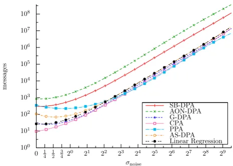
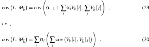
In this section we assume that L satisfies (24). In Fig. 1, the number of messages needed to achieve a success rate of 90% is recorded for each attack mentionned before2. Note
that a success rate threshold has been fixed at 90% but in this configuration each attack can reach 100%.
100 101 102 103 104 105 106 107 108
0 1 4
1 2
3
420 21 22 23 24 25 26 27 28 29
messages
σnoise
SB-DPA AON-DPA G-DPA CPA PPA AS-DPA Linear Regression
Fig. 1: Evolution of the number of messages (y-axis logscaled) to achieve a success rate of 90% according to the noise standard deviation (x-axis logscaled) – Fitted curves.
Curves in Fig. 1 can be split in two parts depending on the noise standard deviation: theoversamplingpart, where a huge number of observations are needed to deal with the important noise effects and theundersamplingpart, where a small number of observations is sufficient. The two situa-tions are analyzed separately in the following. In both cases, the most relevant observations are listed and discussed.
Oversampling. When the noise standard deviation is strictly greater than 23, each distinguisher needs a large number of messages (greater than 500) to reach a success rate of 90%. In this case the curves have the same shape for each dis-tinguisher, which is compliant with the asymptotical results in [6]. Our observations are detailled below:
– The efficiency curves of each attack have the same gra-dient. This suggests us that the noise similarly impacts the efficiency of the attacks.
– The curves corresponding to G-DPA, CPA, PPA, AS-DPA and the regression attack are stacked. Note that with the logscaling that implies that those attacks share
approximatively the same efficiency and that none of them is emerging as better candidate than the others. In fact, in the perfect model scenario, the distinguishers corresponding to these attacks are equivalent to a max-imum likelihood test and the attacks therefore perform in a similar (and optimal) way [6]. This pinpoints the equivalence between the distinguishers when the model function used in the model-based attacks (i.e. , AON-DPA, G-AON-DPA, CPA and PPA) is optimal (i.e., perfectly corresponds to the functionδ(·)in 1).
– As expected, SB-DPA and AON-DPA are less powerful than the others (around 100 and 30 times less efficient than G-DPA, CPA, PPA, AS-DPA and the regression at-tack for the SB-DPA and the AON-DPA respectively). Indeed, by nature they do not exploit all the informa-tion contained in the leakage signal: in SB-DPA only one output bit is targeted over the 8 output bits of the AES, whereas the AON-DPA only exploits a limited part of the leakage measurements.
Remark 5 The good result of G-DPA can be surprizing as the involved model is not the Hamming weight model. The G-DPA model only takes two values -1 and 1 depending on the Hamming weight of the sensitive variable is lower than 4 or not. In fact the linear correlation between the G-DPA model and the Hamming weight model is high (greater than 0.9). That implies an efficiency ratio of 1.2 (0.08 in a log10
scale) according to [21]. This explains why G-DPA’s curve appears stacked with CPA’s curve.
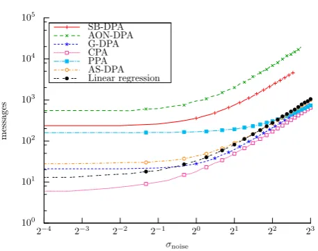
Undersampling. When the noise standard deviation is lower than 23, the number of messages needed to perform an attack is quite small (lower than 500). In this case, the statistical stability of the involved distinguisher plays a role. To better understand how the different attacks perform in this context we redrew in Fig. 2 the curves with a thiner resolution than in Fig. 1. We detail our observations below:
– An important efficiency difference occurs between the CPA, the DPAs and the PPA. For example with a noise standard deviation of 1, CPA needs only 30 messages
100 101 102 103 104 105
2−4 2−3 2−2 2−1 20 21 22 23
messages
σnoise SB-DPA
AON-DPA G-DPA CPA PPA AS-DPA Linear regression
Fig. 2: Evolution of the number of messages (y-axis logscaled) to achieve a success rate of 90% according to the noise standard deviation (x-axis logscaled) – Higher resolu-tion.
to reach a success rate of 90%, whereas PPA needs 280 messages to achieve the same threshold.
– CPA is the most efficient attack. This confirms that Pear-son’s coefficient is the good tool to measure a linear cor-relation.
– In comparison, the PPA is much less efficient than the CPA (and even also than the DPAs). This result was ac-tually expected. Indeed, centering the leakage and the model random variables (i.e.computingEb L·m(Vˆk)
−
b
E(L)Eb m(Vˆk)
instead ofEb L·m(Vkˆ)
in the PPA at-tack) and then normalizing the centered mean by the standard deviations of the random variables (i.e.dividing
b
E L·m(Vˆk)
−Eb(L)Eb m(Vkˆ)
byσb(L)andσb m(Vkˆ)
thus getting the CPA distinguisherCPA(k)ˆ ) is useful to reduce the linear dependency estimation errors when the number of observations is small (i.e. undersampling), which is the case when the attacks are performed for a small amount of noise.
– G-DPA, CPA and PPA are more efficient than AS-DPA and regression attacks. It may be noted that this situation is the opposite of the one occuring in the oversampling case.
al-ways the best attack. However its efficiency is very close to that of G-DPA and PPA when the noise standard deviation reaches the threshold 4. Actually CPA is mainly better than the other tested attacks when the leakage is not very noisy (i.e. , when the noise standard deviation is between 0 and 4). Eventually, it can be noted that the efficiency of AS-DPA and linear regression attack tends to be close to that of the CPA while the perfect model scenario is optimally suited for CPA.
5.2 Attack Results in the Random Linear Leakage Scenario
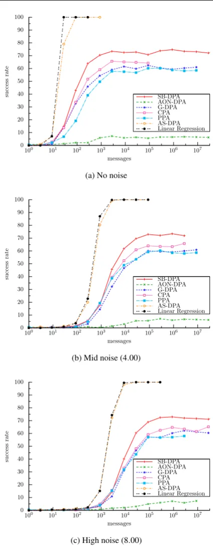
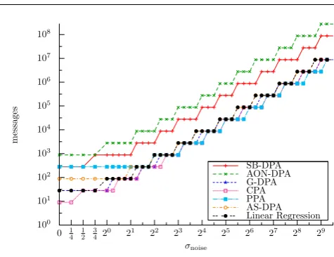
In this section we assume thatLsatisfies (25). In Fig. 3, we recorded the success rate for different numbers of messages and for different values of noise standard deviation.
Observations are reported below. As in the perfect model scenario we can split our observations in two parts.
Oversampling. When the number of messages available is greater than approximately 105×σ2, the curves have the same shape for each distinguisher but contrary to what hap-pened in the perfect model scenario, all the attacks do not reach a success rate of 100%.
– The maximum success rate achieved by the model-based attacks is lower than 75% (e.g. , CPA achieves a suc-cess rate of 62% while G-DPA and PPA are still less efficient with a success rate limit of 58%) independent of the noise standard deviation. In other terms, for some linear functionsδ(·), those attacks do not succeed in dis-criminating the good key candidate when the Hamming weight function is involved as model. In Appendix B, we give a theoretical explanation of the CPA ineffective-ness for some linear functionsδ(·)and we argue that it is related to the algebraic properties of the s-boxSthat is targeted.
– At the opposite, the regression attack and the AS-DPA always succeeds in recovering the key and, actually, in a more efficient way than other attacks. Moreover, as it can be observed in Fig. 3b–3c, this assessment is confirmed independent of the noise standard deviation.
– AON-DPA only reaches a maximal success rate of 6% which is very low compared to the others. A possible explanation for the AON-DPA poor effectiveness resides in the fact that the design of the setsΩ0andΩ1under
the hypothesism=HW is not relevant whenδ(·)is far away from the Hamming weight function
– At the opposite SB-DPA reaches a maximal success rate of 72% which is better than CPA. This observation is not surprising since SB-DPA targets only one bit (indepen-dently of the model choice) over eight, which lowers the impact of the model choice on the remaining seven bits.
0 10 20 30 40 50 60 70 80 90 100
100 101 102 103 104 105 106 107
success
rate
messages
SB-DPA AON-DPA G-DPA CPA PPA AS-DPA Linear Regression
(a) No noise
0 10 20 30 40 50 60 70 80 90 100
100 101 102 103 104 105 106 107
success
rate
messages
SB-DPA AON-DPA G-DPA CPA PPA AS-DPA Linear Regression
(b) Mid noise (4.00)
0 10 20 30 40 50 60 70 80 90 100
100 101 102 103 104 105 106 107
success
rate
messages
SB-DPA AON-DPA G-DPA CPA PPA AS-DPA Linear Regression
(c) High noise (8.00)
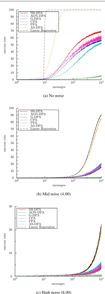
Undersampling. Let us focus on the critic values when a small number of messages is involved in the attack (lower than 500). In this case, the statistical stability of the involved distinguisher plays a role. To better understand how the dif-ferent attacks perform in this context we redrew in Fig. 4 the curves with a thiner resolution than in Fig. 3.
Our observations are detailled below:
– In this situation, each distinguisher has the same ranking as in oversampling.
– G-DPA, CPA and PPA are relatively less efficient than in the perfect model scenario. Indeed, in the latter model scenario they are more efficient than AS-DPA and re-gression attack which is not the case here.
– SB-DPA and AON-DPA still have a different behavior than other model based attacks due to the use of a subop-timal model (with respect to the attacker choice in (22)).
The impact of the noise on the attacks efficiency in our linear random model scenario is very close to what we ob-served in the perfect model context. Namely the maximal success rate is the same whatever the noise deviation but more messages are needed to achieve it. In fact, we confirm the theoretical analysis in [21], where the author shows that doubling the noise deviation just increases the number of needed messages by√Nto reach the same success rate.
Among the attacks we simulated in the random model scenario, the linear regression attack and the AS-DPA are clearly the most efficient ones and they are the only ones that reach a success rate of 100%.
5.3 Attacks Experiments in Real Life
In the previous sections, we have confronted our theoretical analyses with simulations in realistic scenarios. Two attacks emerged, the CPA and the linear regression. In the follow-ing, we aim to confront our results against real measure-ments. Thus we only focus on CPA and linear regression attacks. Attack parameters are described below:
Attacks Target. The 8-bit output of the AES s-box, denoted byS, is targeted. Namely the variableVkin (1) satisfies:
Vk=S(P⊕k) , (26)
wherePcorresponds to an 8-bit value known by the adver-sary.
Attack Types. We list below the attacks we have performed:
– CPA withmsatisfying (22).
– Regression Attack withBlin= (vˆk[i])06i67as basis
func-tions (Assumption 3 withd=1).
– Regression Attack withBquad= (vkˆ[i]·vkˆ[j])06i6j67as
basis functions (Assumption 3 withd=2).
0 10 20 30 40 50 60 70 80 90 100
100 101 102 103
success
rat
e
messages SB-DPA
AON-DPA G-DPA CPA PPA AS-DPA Linear Regression
(a) No noise
0 10 20 30 40 50 60 70 80 90 100
100 101 102 103
success
rat
e
messages SB-DPA
AON-DPA G-DPA CPA PPA AS-DPA Linear Regression
(b) Mid noise (4.00)
0 10 20 30
100 101 102 103
success
rate
messages SB-DPA
AON-DPA G-DPA CPA PPA AS-DPA Linear Regression
(c) High noise (8.00)
Leakage Measurements. Power consumption leakages have been measured on a 8051 8-bit micro-controller. In each measurement curve, the part related to the manipulation of
Vkis composed of 200 points. We suppose the curves to be synchronized (a glitch is used to be synchronized at the be-ginning of the manipulation processing). Before mounting the attacks, a pre-processing step has been performed on the curves to determine the most pertinentpoint of interestfor each attack. By definition, this point is the one among the 200 points per curve that optimizes the attack efficiency. As argued in Section 3.5, it corresponds for the CPA to the point when the error resulting from the approximation of the leak-age by the attack model (i.e.the Hamming weight function) is minimum. For the regression attacks, the point of interest is the point on which the error resulting from the approxima-tion of the leakage by a linear (resp. quadratic) combinaapproxima-tion of the coordinates of the manipulated variable is minimum. During the pre-processing, we have used the fact that we knew the valuesvk,imanipulated by the device. Even if this does not correspond to a real life adversary, pre-processing in this context allows us to determine the time/point when an attack performed by an adversary with no such a knowl-edge is the most efficient. In the following, we sum-up the pre-processing step for the three attacks.
– CPA: the coefficientCPAHW(k)2has been estimated for
each of the 200 points of the curve – the estimation being performed for a sample of size 400,000 – to determine the best attack time.
– Regression Attack: a model functionmlin(resp.mquad)
corresponding to the correct khas been computed for each of the 200 points of the curve, the estimation be-ing performed for a sample of size 400,000. Then, 200 determination coefficientsR2have been performed (one
for each modelMkand the corresponding leakage point) to determine the best attack time corresponding to the basis functionsBlin(resp.Bquad)
Figure 5 illustrates the results of the pre-processing step for each attack and each of the 200 points.
For the attack comparisons, only the point of interest re-sulting in the maximal distinguishing value has been consid-ered for each attack.
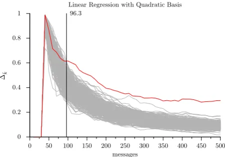
Attack Comparaison. For each attack, the distinguishing co-efficient (iny-axis) has been computed for each key candi-date and for a given (increasing) number of power traces (x -axis). We recorded the minimal number of messages needed to have the real key ranked first (i.e.emerging from others). Results are drawn in Fig. 6,7 and 8. As expected linear re-gression with linear basis is clearly more efficient than CPA
i.e., a lower number of messages is required for the real key to emerge (68 messages is sufficient for the first one while 95 at least are needed for the CPA). As expected, the linear
0 0.05 0.1 0.15 0.2 0.25
0 50 100 150 200
Manipulation times
ρ2(L,mquad(X))
ρ2(L,mlin(X))
ρ2(L,HW(X))
x: 74
y: 0.1670
x: 83
y: 0.2346 xy: 83: 0.2348
Fig. 5: Characterisation Timing Diagram. Max values are pinpointed by an arrow.
regression with quadratic basis needs more messages. In fact the information contained in the quadratic part of the leak-age is not enough to compensate for the increase of noise resulting from the multiplication of leakage points (which is necessary to process the linear regression). Moreover the quadratic regression has to build a larger model (i.e., from a larger basis) from data. We can remark that even with quadratic basis, the minimum number of messages needed to discriminate the real key is still very close to the one for CPA (≈95).
0 0.2 0.4 0.6 0.8 1
0 50 100 150 200 250 300 350 400 450 500
∆ˆk
messages Correlation Factor 95
0 0.2 0.4 0.6 0.8 1
0 50 100 150 200 250 300 350 400 450 500
∆ˆk
messages
Linear Regression with Linear Basis 68
Fig. 7: Evolution of the distinguishing value (y-axis) with the number of messages (x-axis) for all key candidates for linear regression with linear basis. The curve of the real key used in the device is plotted in red.
0 0.2 0.4 0.6 0.8 1
0 50 100 150 200 250 300 350 400 450 500
∆ˆk
messages
Linear Regression with Quadratic Basis 96.3
Fig. 8: Evolution of the distinguishing value (y-axis) with the number of messages (x-axis) for all key candidates for linear regression with quadratic basis. The curve of the real key used in the device is plotted in red.
5.4 Conclusion on the Attack Simulations and Experiments
When the chosen model exactly corresponds to the leak-age function (perfect model case), each distinguisher reveals the key and the CPA and regression attacks are among the most efficient ones (actually except SB-DPA and AON-DPA all tested attacks have equivalent efficiency when the noise increases). Nevertheless in case of undersampling, CPA is ranked first. This can be explained by the fact that the linear regression attack has to rebuild the model from data while CPA is directly provided with the optimal model function and uses the observations only to corroborate a linear de-pendency.
When the model is unknown, the linear regression at-tack and the AS-DPA always succeed in revealing the key. they both are moreover more efficient than the model-based attacks. Nevertheless, collating both, the linear regression is always better than AS-DPA. That is, at a cost of a lit-tle computational overhead, linear regression attack shall be preferred to the other distinguishers.
Finally, if one has a good linear approximation ofδ(·) then CPA is an optimal way to perform an attack. In other cases, the linear regression attack will always perform better.
6 Conclusion and Future Works
In this paper, we have compared standard univariate side channel attacks and we have demonstrated that they all can be rewritten as a CPA. Our analyses show how important the model used for the attacks is. As a good model is not always known to the adversary, we have focused on another sound attack that is not parameterized by a model. This attack (in-troduced by Schindleret al.in [7]) is based on linear regres-sion techniques. It is experimentally compared to CPA both in a favourable context for CPA (i.e., the real leakage model is known) and in a more realistic context (i.e., the real leak-age model is linear but unknown and randomly generated). Eventually we have shown that in all cases the linear regres-sion attack performs well independent of the leakage nature, provided that the key-dependent bits leak independently. We have moreover proposed an extension of the original attack in such a way that the latter assumption can be relaxed.
Based on our study, we think that the linear regression attacks are a relevant alternative to attacks based on ana pri-orimodel choice (ase.g., the CPA). Our work moreover hi-lights the fact that any new attack should be compared at first mathematically and experimentally if needed to the existing ones to reveal the core differences with the state-of-the-art. An interesting extension of our work will be to investigate the behavior of the linear regression attacks in multivariate contexts. Moreover, rewritting the side channel attack prob-lematic in terms of a model estimation probprob-lematic opens the door to a large variety of stochastic tools that could be investigated for further research.
References
1. Kocher, P., Jaffe, J., Jun, B.: Differential Power Analysis. In Wiener, M., ed.: Advances in Cryptology – CRYPTO ’99. Vol-ume 1666 of Lecture Notes in Computer Science., Springer (1999) 388–397