Full Wave Indoor Propagation Modelling Using the Volume
Integral Equation
Ian Kavanagh and Conor Brennan*
Abstract—The transition towards next generation communications has increased the need for fast and accurate propagation models that can predict all aspects of the wireless channel. This paper develops a very accurate approach for indoor propagation modelling based on the volume electric field integral equation (VEFIE). The three-dimensional form of the VEFIE is used to predict frequency domain characteristics. Whilst, a 2D to 3D model is developed based on the 2D VEFIE to perform accurate and efficient time domain predictions. The 2D to 3D model applies correction terms to the solution of the 2D VEFIE to account for three-dimensional propagation. Both models are compared against frequency and time domain measurements as well as popular empirical models for both scenarios.
1. INTRODUCTION
The surge in use of mobile devices in recent times has put a strain on wireless communications infrastructure. This has led to a move towards decentralised networks. Femto and pico cells served by small telecommunications access nodes are becoming more attractive as a means to provide reliable wireless communications networks with a high capacity [1]. These devices are built to work inside buildings and normally provide a small area of coverage but have to serve very complex environments composed of a large variety of different materials [2]. Knowledge of the propagation characteristics of these environments in the frequency and time domains is vital for the continued development of energy efficient wireless communications systems that can provide the required coverage and performance. Thus, there is an increased demand for accurate propagation models that can swiftly describe the propagation channel and serve as tools to optimise the location and configuration of base stations within femto and pico cell environments [3]. These models should be capable of including as much of the geometrical and material information of the environment as is reasonably possible but also yield predictions rapidly. This is extremely challenging for indoor environments.
Empirical or approximate models are presently the most common models used for indoor propagation. They provide rapid predictions but lack the accuracy needed for modern applications. In addition, specific models are intended for either frequency or time domain predictions but not for both. The COST 231 multi-wall model [4] and the Motley-Keenan model [5] are two quick and theoretically simple models for predicting path loss but their accuracy is restricted by the underlying measurement campaigns used to develop them. The SIRCIM computer simulator [6] produces power delay profiles based on statistical channel impulse response models. Significant research has recently been focused on deterministic models, in particular ray tracing, which is built on geometrical optics (GO). Ray tracing is a relatively fast method, although slower than empirical models, that originates from the asymptotic approximation of the solution of Maxwell’s equations at high frequencies. It is capable of producing predictions in both the frequency and time domains. GO has been augmented with the Uniform Theory of Diffraction [7] and diffuse scattering [8] to further augment its accuracy. Diffuse
Received 18 April 2019, Accepted 3 July 2019, Scheduled 17 July 2019
* Corresponding author: Conor Brennan ([email protected]).
scattering has seen significant interest in the literature recently and is increasingly being included in ray tracing models [9, 10]. The current trend, improving the accuracy of ray tracing, suggests that it may be beneficial to take a different approach — to start with an accurate full-wave method and attempt to reduce its computational complexity.
Full-wave propagation models are based on the numerical solution of Maxwell’s equations. Provided that they include all of the information of the propagation problem they should be able to produce accurate predictions but are typically computationally expensive. There have been limited attempts in the literature at developing full 3D propagation models based on full-wave techniques. For example, the finite difference time domain (FDTD) method is shown to be slow for relatively small indoor problems [11, 12] in both 3D and 2D with research ongoing to reduce its computational complexity. The boundary integral equation is another full-wave technique that has been used for indoor propagation [13], while the MR-FDPF method [14, 15] is based on a full-wave technique but employs approximations to significantly reduce its computational cost. These approximations require the MR-FDPF method to be calibrated with measurements before it can be used as an accurate propagation model, thus, calling into question the deterministic nature of the model. The volume electric field integral equation (VEFIE) has previously been investigated for indoor propagation modelling in [16–18] but has not been validated against measurements before for a realistic indoor environment. In this paper, the VEFIE is used as the basis for a full-wave three-dimensional indoor propagation model. The 3D VEFIE and a 2D to 3D model based on the 2D VEFIE are considered. The 3D VEFIE is validated against the Mie Series and the 2D to 3D model is compared against the 3D VEFIE. Both models are applied to realistic building environments and compared against measurements. The 3D VEFIE is applied, primarily, for frequency domain predictions but the 2D to 3D model is used for predictions in both the frequency and time domains. Comparisons against popular empirical models are also presented.
This paper is organised as follows. Section 2 describes the formulation and solution of the VEFIE in three and two dimensions. The 2D to 3D model is presented in Section 3. The measurement campaigns, the results of which are compared against the VEFIE models, are detailed in Section 4. Numerical results analysing the accuracy and runtime of the models as well as comparing them against popular empirical models are presented in Section 5. Section 6 concludes the paper with some final remarks.
2. FORMULATIONS
Indoor propagation modelling can be considered as a general scattering problem governed by Maxwell’s equations. Consider a region of space containing an inhomogeneity with finite volumeV illuminated by an electromagnetic field, with a time dependence of ejωt (assumed and suppressed in the following), located outside of the scatterer as shown in Figure 1. The inhomogeneous scatterer material is characterised by its relative permittivity, r(x, y, z), and conductivity, σ(x, y, z); its permeability is assumed constant and equal to that of free space, i.e., μr(x, y, z) = 1. The volumetric equivalence principle can be used to replace the dielectric material of the scatterer with equivalent induced sources that radiate in free space. The electric field can then be split into two parts: one called the incident field, Ei, due to the primary source and the second denoted the scattered field, Es, produced by the equivalent sources of the scatterer. The total electric field is the superposition of these two fields
E(r) =Ei(r) +Es(r), (1)
which satisfies the vector Helmholtz equation. The total electric field can be represented everywhere by the volume electric field integral equation (VEFIE)
E(r) =Ei(r) +k02
1 + 1
k02
∇∇·
V G(r,r
)χ(r)E(r)dr, (2)
whereG(r,r) is the three-dimensional scalar Green’s function
G(r,r) = e
−jk0|r−r|
4π|r−r|, (3)
and
χ(r) = k 2(r)
k2 0
Figure 1. An inhomogeneous scatterer illuminated by an incident electromagnetic field that produces a scattered electric field. The fields in the vicinity of the scatterer must satisfy Maxwell’s equations.
is the contrast function, the use of which incorporates the geometry of the problem. k0is the background (free space) wave number and k2(r) = ω2μ(r)(r)−jωμ(r)σ(r). In this work, the primary unknown is chosen to be the electric field, E(r), as opposed to the volume currents, J(r), because although it increases the size of the computational domain it enables the use of the fast Fourier transform (FFT) to expedite its solution. The electric field is related to the volume currents by
J(r) =jω0[r(r)−1]E(r). (5)
The ease with which inhomogeneous scatterers can be modelled and the absence of a need for absorbing boundary conditions, such as are needed in an FDTD implementation, make this a very convenient method.
The 2D VEFIE is derived from Eq. (2) by assuming that the problem is homogeneous in the z -direction, i.e., infinite scatterers, and invariant fields, and transverse magnetic (TMz) polarisation. This yields
Ez(r) =Ezi(r) +k02
SG(r,r
)χ(r)E
z(r)dr. (6)
It can be shown that Eq. (3) reduces to the two-dimensional scalar Green’s function given by
G(r,r) = 1 4jH
(2) 0
k0|r−r|
, (7)
where H0(2)(k0|r−r|) is the zeroth order Hankel function of the second kind. [16] demonstrates the suitability of the two-dimensional VEFIE for the problem of indoor propagation modelling, which is extended to three dimensions in this work.
2.1. Incident Field
In a full 3D problem described by Eq. (2), the primary source is modelled in three dimensions. Throughout this work, a vertical Hertzian dipole (oriented along thez-direction) is used for this purpose. Its far-field radiation pattern is described by
Ei(r)∼= ˆθjωμ0 Il 4πre
−jk0rsinθ, (8)
In two dimensions, for problems described by the 2D VEFIE in Eq. (6), the source is modelled as two-dimensional. The dipole fields in Eq. (8) are replaced with those of a line source
Ezi(r) = 1 4jH
(2)
0 (k0r). (9)
For the purposes of comparison the 2D fields computed using the line source are assumed to be in the plane perpendicular to the centre of the axis of the Hertzian dipole, i.e., forθ= π2 and z= 0.
2.2. Discretisation
The solutions of both Eqs. (2) and (6) proceed similarly. The problem to be solved is discretised into
N uniform cells of size Δv = Δx×Δy×Δz in 3D [19] and size Δx×Δy in 2D [20]. The unknown total electric field is approximated by the superposition ofN pulse basis functions and point-matching is employed to enforce the resultant equations at the cell centres. This results in a matrix equation of the form
V=ZE, (10)
for both the 3D and 2D VEFIE.
In the discretised version of the 3D VEFIE, Eq. (2),Z is a matrix of size 3N ×3N which can be expressed as
Z=I−k20ΔvGD−ΔvHGD. (11)
E and Vare column vectors of length 3N representing the unknown total electric field and the known incident electric field respectively, that is
E= ⎡ ⎣EExy
Ez
⎤
⎦, V= ⎡ ⎢ ⎣
Eix Eiy Eiz
⎤ ⎥
⎦. (12)
Eμ and Eiμ, where μ = {x, y, z}, in Eq. (12) are vectors of length N and contain the x, y, and z
components of the total and incident electric fields at the centre of each cell in the discretised problem.
I is the identity matrix, Grepresents the Green’s function in Eq. (3)
G= ⎡
⎣G0T G0T 00
0 0 GT
⎤
⎦, (13)
where each GT has dimensions N ×N and block Toeplitz structure. D is a diagonal contrast matrix consisting of Eq. (4) evaluated at the cell centres. His a sparse matrix containing a suitable numerical implementation of the ∇∇·operation.
For the discretised form of the 2D VEFIE, Eq. (6),Zis a matrix of sizeN×N given by
Z=I−k20GD. (14)
E and V are column vectors of length N representing the z component of the unknown total electric field and the known incident electric field in two dimensions respectively. I is the identity matrix, G
represents the two-dimensional Green’s function in Eq. (7), which exhibits block Toeplitz structure, and
D is a diagonal matrix similar to the 3D case above.
2.3. Solution
cases the bi-conjugate gradient stabilised (BiCGSTAB) [22] method is used to solve Eq. (10) for the unknown total electric field.
The choice to use the total electric field as opposed to the volume currents in the derivation of the VEFIE is very important for accelerating its solution. The product ofGwithDEis a convolution due to the Toeplitz structure of Gin both three and two dimensions which can be exploited by using the FFT to efficiently compute the product of Gwith DE. This reduces the complexity of computing this matrix-vector product during each iteration of the iterative solver fromO(N2) toO(NlogN). The storage requirements for G are also reduced from O(N2) to O(N) as all that is required to specify G
is a single N ×1 vector. DE can also be computed efficiently because D is a sparse diagonal matrix which also only requires a single N×1 vector to specify it. MultiplyingD withE can be performed as a vector-vector multiplication instead of a matrix-vector product reducing its complexity from O(N2) to O(N).
The use of the total electric field as the primary unknown in the VEFIE enables the use of the FFT, but it requires the discretisation of the entire problem domain including free space. This greatly increases the number of unknown values that need to be computed. However, by considering the underlying structure of the matrix elements it is easy to distinguish between unknown values that have an effect on unknowns located elsewhere in the problem and those that do not due to being located in free space where Eq. (4) equals zero. Such unknown values in free space consequently do not affect the solution at any other location. Thus, a reduced operator can be used to ignore unknown values in free space, while still retaining the grid structure necessary for the implementation of the FFT. This reduces the number of iterations required to converge to a solution. This technique is described in more detail in [23].
2.4. Validation with Mie Series
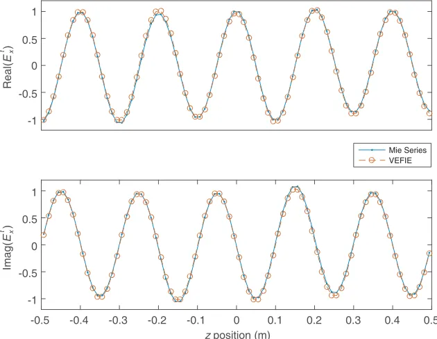
To validate the 3D VEFIE the analytical Mie Series solution for scattering from a homogeneous sphere is used. A dielectric sphere of radius 0.2470 m with relative permittivityr = 2.62 is placed in free space in the presence of a plane wave travelling in thez-direction and polarised in thex-direction at 1.5 GHz. A very good agreement is achieved between the analytical Mie Series result and the 3D VEFIE as shown in Figure 2, validating its implementation.
Real(
E
)
t x
-1 -0.5 0 0.5 1
Mie Series VEFIE
z position (m)
-0.5 -0.4 -0.3 -0.2 -0.1 0 0.1 0.2 0.3 0.4 0.5
Imag(
E
)
-1 -0.5 0 0.5 1
t x
3. 2D TO 3D MODEL
The solution of the 3D VEFIE is quite computationally expensive compared with the 2D formulation. This is for two reasons. Firstly, the solution of the 3D VEFIE requires the computation of three field components,x,y and z, as opposed to the singlez component in the 2D case. Secondly, assuming that
Nx, Ny and Nz are the number of discretisations in the x, y and z-directions respectively, the total number of discretisations required grows asNxNyNz instead of NxNy in the two-dimensional problem. This shows that a more computationally efficient approach would be to develop a model based on the 2D VEFIE and correct its solution to account for three-dimensional propagation. A simple heuristic technique to approximately correct the solution of the 2D VEFIE is presented here. This leads to an accurate 3D propagation model capable of providing a solution in a fraction of the time required for a full 3D solution.
3.1. Correction Method
There are several differences between the 3D and 2D forms of the VEFIE. Due to the use of the dipole and line source for the incident fields the main difference present in both the incident and scattered fields arises from the reduction of
e−jk0rx,y,z
4πrx,y,z ,
to its 2D representation
1 4jH
(2)
0 (k0rx,y)≈ 1 4j
2j πk0rx,ye
−j k0rx,y,
where
2j
πk0re−jk0r is the large argument approximation of the zeroth order Hankel function. rx,y,z denotes three-dimensional distance andrx,y two-dimensional distance, i.e., zis assumed to be 0. If the solution of the 2D VEFIE is chosen as the plane perpendicular to the centre of the axis of the Hertzian dipole, θ = π2, then a partial correction for the 2D fields in this plane to account for 3D propagation can be achieved through multiplication by
k0
2πrx,y,z. (15)
It has been found experimentally that a reasonable correction for the 2D field forθ= π2 can be obtained through multiplication of a modified version of Eq. (15) given by
β
√
rx,y,z, (16)
where
β = ωμ0Il
4
k0
2π, (17)
and I and lare the same as that in Eq. (8).
The base correction for the 2D VEFIE is, thus, given by
Et(rx,y,z) = βE√z(rx,y)
rx,y,z , (18)
where Et(rx,y,z) is the total field in three dimensions, and Ez(rx,y) is the solution of the 2D VEFIE.
Et(rx,y,z) is a good approximation for the 3D fields as the dominant component in the 3D VEFIE is
the z component. The fields at planes when θ= π2 can be computed by splitting them up into those that have line of sight (LOS) of the antenna and those that do not (NLOS). For points in LOS, the 3D fields can be computed by
Et(rx,y,z) =βE√z(rx,y)
where
γ = tan−1
x2
a+y2a
|za|
, (20)
wherexa,ya, andzaare the distances in thex,y, andz-directions to the pointrx,y,zfrom the transmitter. sin(γ) applies a correction based on the radiation pattern of the antenna because this is the dominant component in indoor LOS scenarios. Points in NLOS regions are computed with
Et(rx,y,z) =α+βE√zr(rx,y)
x,y,z , (21)
whereα, which has been experimentally determined, is given by
α= za
10. (22)
3.2. Comparison against 3D and 2D VEFIE
Consider a cube of size 2 m×2 m×2 m consisting of a concrete-like material defined byr= 4, μr= 1 andσ= 0.01 positioned in air with its top left edge located at (−0.5,1.5) and centred in thez-direction, i.e., it extends fromz=−1 to z= 1. The transmitter is located at (−1.5,2,0). Figure 3 demonstrates a comparison between the 2D to 3D model and the 3D and 2D VEFIE at a frequency of 1.2 GHz along thez axis from z=−1 to z= 1. The LOS results located at (−2,−1, z), whilst the NLOS results are for the locations (2,−1, z). The RMS error and standard deviation for the results in Figure 3 can be found in Table 1.
-1 -0.8 -0.6 -0.4 -0.2 0 0.2 0.4 0.6 0.8 1
z location (m)
-60 -55 -50 -45 -40 -35 -30 -25 -20
Received power (dBm)
3D VEFIE-LOS 2D to 3D-LOS 2D VEFIE-LOS
3D VEFIE-NLOS 2D to 3D-NLOS 2D VEFIE-NLOS
Figure 3. Comparison of the 2D to 3D model against the 3D and 2D VEFIE. The location of the LOS results is (−2,−1, z) and the NLOS results are located at (2,−1, z).
Table 1. Accuracy of the 2D to 3D model and 2D VEFIE against the 3D VEFIE for the results in Figure 3.
LOS NLOS
RMS Error Std. Dev. RMS Error Std. Dev
2D VEFIE 9.06 1.21 13.73 4.37
2D to 3D 1.68 1.02 3.19 3.11
0.5 1 1.5
Frequency (GHz)
-100 -80 -60 -40 -20
Received power (dBm)
(2, -1, 0)
0.5 1 1.5
-50 -40 -30 -20
-10 (-2, -1, 0)
0.5 1 1.5
Frequency (GHz)
-100 -80 -60 -40
-20 (2, -1, 1)
3D VEFIE 2D to 3D 2D VEFIE
0.5 1 1.5
-50 -40 -30 -20
-10 (-2, -1, -1)
Figure 4. Comparison of the 2D to 3D model against the 3D and 2D VEFIE over a frequency range from 500 MHz to 1.5 GHz with a spacing of 10 MHz.
Table 2. Averaged accuracy of the 2D to 3D model and 2D VEFIE against the 3D VEFIE for the results in Figure 4.
LOS NLOS
RMS Error Std. Dev. RMS Error Std. Dev
2D VEFIE 9.65 2.95 19.32 5.51
2D to 3D 2.44 2.45 3.16 3.01
wide frequency range due to its derivation from the full 3D VEFIE. Figure 4 and Table 2 demonstrate the effectiveness of the 2D to 3D model over a frequency range from 500 MHz to 1.5 GHz. Figure 4 compares the 2D to 3D model against the 3D and 2D VEFIE from 500 MHz to 1.5 GHz at the points (−2,−1,0), (2,−1,0), (−2,−1,−1), (2,−1,1). The average RMS error and standard deviation for all of these results are shown in Table 2. These results include points in LOS, NLOS, points in the same plane as the transmitter and points in a plane 1 m above and below the transmitter but in each case the 2D to 3D model provides a much better agreement with the 3D VEFIE than the 2D VEFIE. The good agreement achieved by the 2D to 3D model across a range of frequencies (Figure 4) suggests an ability to produce accurate time domain simulations, by applying an inverse Fourier transform to this data. This is explored more in Section 5.3.
3.3. Limitations
is assumed. However, this is a good approximation for the total field in 3D as it is dominated by thez
component. The derivation here is specific to a vertical dipole but works well for other omni-directional antennas that have a similar radiation pattern to a dipole as shown in Section 5.3.
4. MEASUREMENT CAMPAIGNS
Two measurement campaigns are used to validate and determine the accuracy of the VEFIE based models. The first measurement campaign was carried out on a single floor in a portion of a typical house. It measured the received signal strength for several receiver locations. The second campaign was carried out in a laboratory room at the Graz, University of Technology [24] where the complex channel transfer function was measured.
4.1. Narrow Band Campaign
The first measurement campaign measured the received signal strength in the building depicted by the 2D slice shown in Figure 5. The portion of the building where the campaign was performed is of size 6.95 m×8.2 m×2.95 m. In the 2D slice shown and for the purposes of applying the 2D VEFIE to the problem the only materials present are those shown in Figure 5, i.e., concrete, glass and wood. The floors in the house are wood, stone and tile for the living room, hall and bathroom respectively. The ceiling is a thin layer of plaster in each room. The electrical parameters used to model these materials can be found in Table 3. They are based on averaged values from the literature around 915 MHz. Small clutter such as a coffee table, book cabinet and chairs have been neglected in the model but are present in the measurement environment. The stairs located on the left hand side of the building, as seen in Figure 5, are modelled as a solid block of wood. These discrepancies between the model and measurement environment will introduce a source of error in the results. Currently, there has been no investigation of the level of detail required by indoor propagation models.
This measurement campaign used two LSR 900 MHz omnidirectional dipole antennas operating at 915 MHz and an Anritsu MS2651B spectrum analyser to measure the received signal strength. At each receiver location shown in Figure 5 five measurements were taken; one at the receiver location and the
Table 3. Material parameters used to characterise the house in Figure 5.
Material r μr σ
Concrete 4.4 1 0.01
Glass 4.8 1 0
Wood 2.2 1 0
Stone 4.0 1 0.1
Tile 12 1 0
Plaster 2.5 1 0
remaining four at the corners of aλ×λsquare centred on the receiver location. These five measurement values were averaged to remove some of the effects of fast fading on the results.
4.2. Wide-Band Campaign
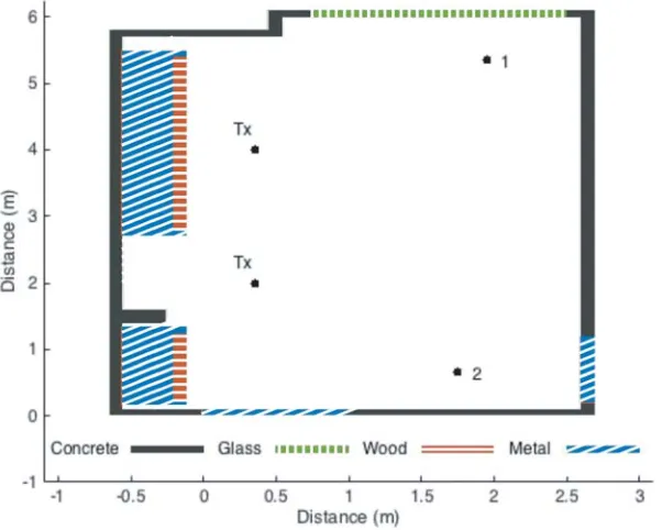
The second measurement campaign measured the complex channel transfer function for the room shown in Figure 6. The size of the room is 3.35 m×6.1 m. It is made up of four different materials, namely concrete, glass, wood and metal. The electrical parameters used to model these are shown in Table 4. These are based on values reported by Meissner et al. in [25] and averaged values from the literature for wood and metal (assumed to be aluminium). Only the 2D VEFIE and 2D to 3D model are applied to this building, therefore, the height, floor and ceiling are neglected for modelling purposes. As well, there are tables on the right hand side of the room that are neglected which will introduce a source of error in the comparison between the measurements and VEFIE models. Skycross SMT-3TO10M UWB antennas and custom made coin antennas which both have an approximately uniform azimuthal radiation pattern and zeros in the pattern at +/−90◦ elevation angle [24] were used. The complex channel transfer function over the frequency range from 3.1 GHz to 10.6 GHz was measured using a Rohde and Schwarz ZVA-24 vector network analyser [24].
Table 4. Material parameters used to characterise the room in Figure 6.
Material r μr σ
Concrete 6.0 1 0.08
Glass 5.5 1 0
Wood 2.2 1 0
Metal 1.7 1 3×10⁷
5. NUMERICAL RESULTS
In this section the VEFIE based models are compared against the measurement campaigns described in Section 4 and popular empirical models. The accuracy of the models is examined in the frequency domain for the 3D and 2D VEFIE and in the frequency and time domains for the 2D to 3D model.
5.1. Frequency Domain Measurement Comparison
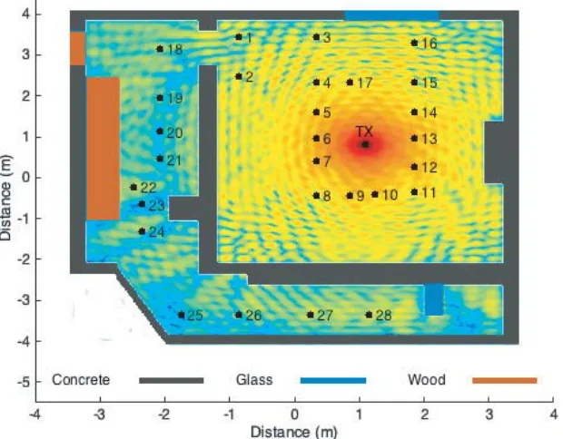
The 3D and 2D VEFIE are applied to the propagation problem defined by the house shown in Figure 5. Their solution produces a value for the total electric field at every discretised point within the problem. Figure 7 demonstrates the result of the 3D VEFIE solution at a height of 1.39 m above the floor. This is the same height as the transmitter and receivers. The results of the 3D and 2D VEFIE are averaged over a box of sizeλ×λcentred on the receiver location, similar to the averaging applied to the measurements to reduce the effect of fast fading. A comparison of the VEFIE against the measurement results is shown in Figure 8. The root mean square (RMS) error and standard deviation between the VEFIE and measurements are shown in Table 5. The 3D VEFIE agrees very well with the measurement results. The 3D VEFIE agrees very well with the analytical Mie Series solution as shown in Section 2.4, thus, the discrepancies between the 3D VEFIE and measurement results can be accounted for by an incomplete knowledge of the environment and the lack of clutter included in the simulation, like tables
Table 5. Runtime and accuracy measurements of the 3D and 2D VEFIE and 2D to 3D model.
Runtime (mins) RMS Error (dB) Std. Dev. (dB)
3D VEFIE 1168 3.81 3.87
2D VEFIE 1.6 28.60 5.00
2D to 3D 1.6 4.39 4.23
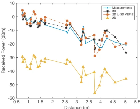
and chairs. As noted in Section 4.1 the measurement environment contains a coffee table, book case, and chairs that are not modelled. The stairs are also modelled as a solid block of wood. However, it is clear from Figure 8 and Table 5 that the 2D VEFIE requires a correction term to account for 3D propagation and to be able to provide a good agreement with the 3D VEFIE and consequently the measurement results.
0.5 1 1.5 2 2.5 3 3.5 4 4.5 5 5.5
Distance (m) -60
-50 -40 -30 -20 -10 0 10
Received Power (dBm)
Measurements 3D 2D to 3D VEFIE 2D
Figure 8. Comparison of the 3D and 2D VEFIE and the 2D to 3D model against measurements for the problem shown in Figure 5.
The 2D to 3D model presented in Section 3 provides corrections that when applied to the 2D VEFIE correct its solution to account for three-dimensional propagation. The results of this model are also shown in Figure 8 against the VEFIE and measurements. It can clearly be seen the 2D to 3D model provides a significant improvement over the 2D VEFIE. The full 3D VEFIE solution is more accurate than the 2D to 3D model. However, the main advantage of the 2D to 3D model is its significantly quicker runtime, 1.6 minutes as opposed to 1,168 minutes for the full 3D VEFIE. It should be noted that the runtime of the 2D to 3D model is dependant on the efficiency of the visibility algorithm used to determine whether points are in LOS or NLOS regions. Here, the visibility is known for the 28 receiver points and thus the additional time to compute the 2D to 3D model over the 2D VEFIE is negligible.
5.2. The 3D VEFIE and Empirical Models
5.2.1. COST 231 Multi-Wall Model
The single floor COST 231 multi-wall model [4] represents the path loss as
P L(d) =L0+ 20 log10(d) + kw
i=1
kwiLwi, (23)
wheredis the distance from the transmitter, andkw is the number of different types of walls, two being used in this work. kwi is the number of walls of type Lwi obstructing the field, and Lwi is 3.4 dB for light walls (<10 cm) and 6.9 dB for heavy walls (>10 cm). L0 is fitted to the measurements.
5.2.2. Adjusted Motley-Keenan Model
The adjusted Motley Keenan model [5] calculates the path loss as
P L(d) =L0+ 10nlog10(d) + N
i=1
kiL0i2 log3
ei e0i
, (24)
where dis the distance from the transmitter; ki is the number of walls of typei;L0i is the loss in the reference wall of typei;e0iis the thickness of the reference wall of typei; andeiis the actual thickness of the wall. nmust be determined experimentally by performing measurement campaigns. The reference values required for the adjusted Motley-Keenan model can be found in Table 6. L0 and nare fitted to the measurements using a least squares approach.
Table 6. Reference values for Motley-Keenan model.
Wall e0i(cm) L0i(dB)
Plasterboard 12 2.5
Concrete 15 6.0
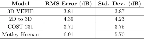
The RMS error and standard deviation of the COST 231 multi-wall model and the adjusted Motley-Keenan model are shown in Table 7. It can be seen in Figure 9 the empirical models fit a curve through the measurement results with a few variations to account for NLOS areas. They do not include the fading information present in the 3D VEFIE and 2D to 3D model. Each of the empirical models has to be fitted to the measurement results. They require L0 to be determined experimentally. The Motley-Keenan model requires a measurement campaign to determine the value of n also. The 3D VEFIE and 2D to 3D model do not require measurement campaigns to be able to provide a very high level of accuracy but they do require knowledge of the environment, the scattering objects that are present and the electrical parameters used to characterise them, permeability, permittivity and conductivity. As well as producing a low RMS error and standard deviation the 3D VEFIE and 2D to 3D model can be used to produce information about the signal in the time domain and angle of arrival information also [29].
Table 7. RMS error and standard deviation of the 3D VEFIE, 2D to 3D model and empirical models.
Model RMS Error (dB) Std. Dev. (dB)
3D VEFIE 3.81 3.87
2D to 3D 4.39 4.23
COST 231 3.71 3.75
0.5 1 1.5 2 2.5 3 3.5 4 4.5 5 5.5 Distance (m)
-35 -30 -25 -20 -15 -10 -5 0 5
Received Power (dBm)
Measurements 3D 2D to 3D COST 231 Multi-Wall Motley-Keenan
Figure 9. Comparison of the 3D VEFIE, 2D to 3D model and empirical models against measurements.
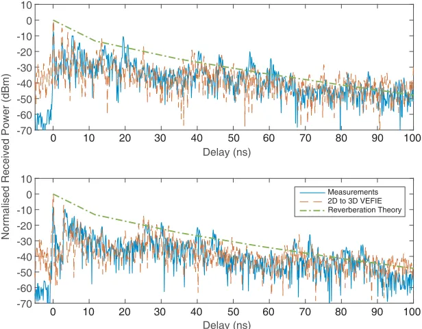
5.3. Time Domain Analysis
A complete indoor propagation model should be capable of predicting the radio channel in both the frequency and time domains accurately and efficiently. The 2D to 3D model presented has been shown to work well for frequency domain predictions. Now, the 2D to 3D model is applied to the room in Figure 6 for the separate transmitter locations shown, (0.35,2) and (0.35,4), and solved from 3.1 GHz to 10.6 GHz at 5 MHz increments. Time domain results are computed from the frequency sweep information by applying the inverse discrete Fourier transform (DFT) which produces a power delay profile (PDP) like those shown in Figure 10. Due to the periodicity of the DFT the data for the 2D to 3D model and measurements is windowed with a Hann window before the DFT is applied to it in order to reduce the effect of aliasing on the resultant time domain data. In Figure 10 the 2D to 3D model is compared
Delay (ns) -70
-60 -50 -40 -30 -20 -10 0 10
Normalised Received Power (dBm)
Delay (ns) -70
-60 -50 -40 -30 -20 -10 0 10
Measurements 2D to 3D VEFIE Reverberation Theory
0 10 20 30 40 50 60 70 80 90 100
0 10 20 30 40 50 60 70 80 90 100
against the measurement results where it can be seen that except for the noise preceding the initial pulse a good agreement is achieved. There are errors expected between the 2D to 3D model results and the measurements due to the incomplete modelling of the environment as noted in Section 4.2. There are tables and other small items that are not included in the model which will affect the measurement results. The 2D to 3D model results are also compared against a simpler model based on reverberation theory [30] in Figure 10. The model based on reverberation theory considers the volume of the room, the surface area of the walls, floor and ceiling as well as their material properties to compute an average power delay profile for the entire room. Similar to the empirical models investigated in Section 5.1 the reverberation theory model fits a curve through the measurement results for the specific transmitter and receiver locations investigated here. The 2D to 3D model provides a better accuracy that can also be seen in a comparison of the most commonly used metrics, namely mean delay and RMS delay spread shown in Table 8. Once all of the 2D simulations have been performed information about the total electric field is available at every frequency for every discretised point within the 2D problem. Thus a power delay profile can be computed for every receiver point without any extra significant overhead. A big advantage of the 2D to 3D model approach is the finer level of detail that it provides in the resultant PDP as shown in Figure 10 as well as the more accurate mean delay and RMS delay spread values.
The 2D to 3D time domain modelling approach produces a large amount of data. In the frequency domain analysis, the data from the VEFIE and measurement campaign was averaged over a box of size
λ×λto remove some of the effects of fast fading. Here, by applying a 10-point moving average filter, which corresponds to a delay of 1 ns, a much clearer picture of the signal evolution is shown as can be seen in Figure 11.
Table 8. Average mean delay and RMS delay spread for all transmitter and receiver pairs.
Mean Delay (ns) RMS Delay Spread (ns)
Measurements 51.86 28.68
2D to 3D 51.65 28.65
Reverberation Theory 55.16 36.51
-70 -60 -50 -40 -30 -20 -10 0
Normalised Received Power (dBm)
-70 -60 -50 -40 -30 -20 -10 0
Measurements 2D to 3D VEFIE Delay (ns)
Delay (ns)
0 10 20 30 40 50 60 70 80 90 100
0 10 20 30 40 50 60 70 80 90 100
6. CONCLUSIONS
The current state of wireless system development and indoor location and tracking algorithms have created a greater demand for very accurate indoor propagation models. In this paper the volume electric field integral equation (VEFIE) is used as the basis for complete indoor propagation modelling in the frequency and time domains. The three-dimensional formulation of the VEFIE is applied for modelling in the frequency domain. The 2D VEFIE despite its speed is shown to lack accuracy. Novel heuristic correction terms are applied to the 2D VEFIE to correct its solution and account for 3D propagation. This model, called the 2D to 3D model, can be applied for modelling in the frequency and time domains due to its speed and high level of accuracy. The two approaches; the 3D VEFIE and 2D to 3D model, are compared against measurements taken within a single floor of a house where they show a high level of accuracy. The 2D to 3D model is also used to predict time domain information for a laboratory room and compared against measurements. In both comparisons with measurements the VEFIE based models are also compared against popular empirical models where they show a higher level of accuracy and increased detail.
ACKNOWLEDGMENT
The authors gratefully acknowledge the financial support offered by the Irish Research Council under the Government of Ireland Postgraduate Scholarship Scheme 2014. The authors would like to thank the Wireless Communications Group of the Signal Processing and Speech Communications Laboratory at Graz, University of Technology for providing access to their MeasureMINT UWB database.
REFERENCES
1. Zhang, J., G. De la Roche, et al.,Femtocells: Technologies and Deployment, Wiley Online Library, 2010.
2. Saunders, S. and A. Arag´on-Zavala, Antennas and Propagation for Wireless Communication Systems, John Wiley & Sons, 2007.
3. Rappaport, T. S., Wireless Communications: Principles and Practice, Vol. 2, Prentice Hall PTR, New Jersey, 1996.
4. Pedersen, G. F.,COST 231 — Digital Mobile Radio towards Future Generation Systems, EU, 1999. 5. Motley, A. J. and J. M. P. Keenan, “Personal communication radio coverage in buildings at 900 MHz
and 1700 MHz,” Electronics Letters, Vol. 24, No. 12, 763–764, Jun. 1988.
6. Rappaport, T. S., S. Y. Seidel, and K. Takamizawa, “Statistical channel impulse response models for factory and open plan building radio communicate system design,” IEEE Transactions on Communications, Vol. 39, No. 5, 794–807, May 1991.
7. De Adana, F. S., O. G. Blanco, I. G. Diego, J. P. Arriaga, and M. F. Catedra, “Propagation model based on ray tracing for the design of personal communication systems in indoor environments,” IEEE Transactions on Vehicular Technology, Vol. 49, No. 6, 2105–2112, Nov. 2000.
8. Ament, W. S., “Toward a theory of re ection by a rough surface,” Proceedings of the IRE, Vol. 41, No. 1, 142–146, Jan. 1953.
9. Degli-Esposti, V., “A diffuse scattering model for urban propagation prediction,” IEEE Transactions on Antennas and Propagation, Vol. 49, No. 7, 1111–1113, Jul. 2001.
10. Degli-Esposti, V., D. Guiducci, A. de’Marsi, P. Azzi, and F. Fuschini, “An advanced field prediction model including diffuse scattering,” IEEE Transactions on Antennas and Propagation, Vol. 52, No. 7, 1717–1728, Jul. 2004.
11. Zhai, M.-L., W.-Y. Yin, Z. D. Chen, H. Nie, and X.-H. Wang, “Modeling of ultra-wideband indoor channels with the modified leapfrog ADI-FDTD method,” International Journal of Numerical Modelling: Electronic Networks, Devices and Fields, Vol. 28, No. 1, 50–64, 2015.
13. Lim, C.-P., J. L. Volakis, K. Sertel, R. W. Kindt, and A. Anastasopoulos, “Indoor propagation models based on rigorous methods for site-specific multipath environments,” IEEE Transactions on Antennas and Propagation, Vol. 54, No. 6, 1718–1725, Jun. 2006.
14. De la Roche, G. and J. M. Gorce, “A 3D formulation of MR-FDPF for simulating indoor radio propagation,” 2006 First European Conference on Antennas and Propagation, 1–6, Nov. 2006. 15. De la Roche, G., J. M. Gorcey, and J. Zhang, “Optimized implementation of the 3D MR-FDPF
method for indoor radio propagation predictions,”2009 3rd European Conference on Antennas and Propagation, 2241–2245, Mar. 2009.
16. Pham-Xuan, V., I. Kavanagh, M. Condon, and C. Brennan, “On comparison of integral equation approaches for indoor wave propagation,” 2014 IEEE-APS Topical Conference on Antennas and Propagation in Wireless Communications (APWC), 796–799, Aug. 2014.
17. Kavanagh, I., “Developing a method of moments based indoor propagation model,” EUROCON 2015 — International Conference on Computer as a Tool (EUROCON), Vol. 1, No. 2, 1–6, IEEE, Sep. 2015.
18. Lu, C. C., “Indoor radio-wave propagation modeling by multilevel fast multipole algorithm,” Microwave and Optical Technology Letters, Vol. 29, No. 3, 168–175, 2001.
19. Zhang, Z. Q., Q. H. Liu, C. Xiao, E. Ward, G. Ybarra, and W. T. Joines, “Microwave breast imaging: 3-D forward scattering simulation,” IEEE Transactions on Biomedical Engineering, Vol. 50, No. 10, 1180–1189, Oct. 2003.
20. Peterson, A. F., S. L. Ray, and R. Mittra, Computational Methods for Electromagnetics, Vol. 2, IEEE Press, New York, 1998.
21. Golub, G. H. and C. F. van Loan,Matrix Computations, Vol. 3, JHU Press, 2012.
22. Van der Vorst, H. A., Iterative Krylov Methods for Large Linear Systems, Vol. 13, Cambridge University Press, 2003.
23. Van Dongen, K., C. Brennan, and W. M. D. Wright, “Reduced forward operator for electromagnetic wave scattering problems,” IET Science, Measurement and Technology, Vol. 1, No. 1, 57–62, Jan. 2007.
24. Meissner, P., E. Leitinger, S. Hinteregger, J. Kulmer, M. Lafer, and K. Witrisal,
“MeasureMINT UWB database, Graz University of Technology,” [online] available:
www.spsc.tugraz.at/tools/UWBmeasurements, 2013.
25. Meissner, P., M. Gan, F. Mani, E. Leitinger, M. Frhle, C. Oestges, T. Zemen, and K. Witrisal, “On the use of ray tracing for performance prediction of UWB indoor localization systems,” 2013 IEEE International Conference on Communications Workshops (ICC), 68–73, Jun. 2013.
26. Sarkar, T. K., Z. Ji, K. Kim, A. Medouri, and M. Salazar-Palma, “A survey of various propagation models for mobile communication,” IEEE Antennas and Propagation Magazine, Vol. 45, No. 3, 51–82, Jun. 2003.
27. Solahuddin, Y. F. and R. Mardeni, “Indoor empirical path loss prediction model for 2.4 GHz 802.11n network,” 2011 IEEE International Conference on Control System, Computing and Engineering (ICCSCE), 12–17, Nov. 2011.
28. Andrade, C. B. and R. P. F. Hoefel, “IEEE 802.11 WLANs: A comparison on indoor coverage models,”2010 23rd Canadian Conference on Electrical and Computer Engineering (CCECE), 1–6, May 2010.