Available Online atwww.ijcsmc.com
International Journal of Computer Science and Mobile Computing
A Monthly Journal of Computer Science and Information Technology
ISSN 2320–088X
IMPACT FACTOR: 6.199
IJCSMC, Vol. 8, Issue. 7, July 2019, pg.52 – 64
Selection of Optimal Materialized Views in
Data Warehouse Using Hybrid Technique
Wesal Adeeb Abdullah
1; Naji Mutar Sahib
2; Jamal Mustafa Al-Tuwaijari
31
Department of Computer Sciences, College of Science, Diyala University, Iraq 2
Department of Computer Sciences, College of Science, Diyala University, Iraq 3
Department of Computer Sciences, College of Science, Diyala University, Iraq 1 [email protected],2[email protected], 3[email protected]
Abstract— Decision making is the main purpose of DW. Typically, decision making queries are analytical, complex, recurring and include aggregation functions or many join operations posed over DW. A critical issue in designing DW is answering these queries efficiently. Many ways have been proposed to address this problem, one of them is materialize views while due to space constraints all views cannot be materialized in DW. In this paper we have design an efficient methodology for selecting an optimal MVs based on three factors (MV response time, MV storage area and MV frequency) using bitmap index to minimize the total time of creating MVs, then using hybrid technique (Firefly algorithm and Quantum Particle Swarm Optimization algorithm) to select optimal MV which has low response time, low storage area and high frequency. The results proved that bitmap index achieved good results because it take less time and storage area in recoupoing results since bitmap indices have the ability of accomplishing processes on index level before recouping the base relations where, the total time of applying these functions over bitmap index was found 168 milleseconds, while directly over base tables was found 216 milleseconds. Also, the hybrid technique was more efficient in term of optimal MVs selection time since, FA presents optimal initial point to QPSO algorithm.
Keywords— data warehouse, materialized views, processing time, firefly algorithm, quantum particle swarm optimization algorithm.
I. INTRODUCTION
rapidly [4]. Selecting views to materialize is one of the most significant decisions in DW design. The problem of view selection can be defined as select a collection of derived views which decrease the total query processing time to materialize them in DW. Therefore the goal is select an appropriate collection of views to materialize to decrease the total query processing time [3]. In this paper MVs are selected under three constraints (MV response time, MV storage area and MV frequency). Another alternative method to access data which required much less time in DW is bitmap index technique, since it is efficient especially for read-mostly data. Bitmap indices in most DW applications are shown to perform good results than other indexing schemas like: B-tree or R-tree [5].
II. RELATEDWORKS
Sapna and Roshna in 2014 [4] proposed framework for achieving high query performance by detecting which query is more beneficial for creating the MVs. They determine the performance of any query depending on the processing time required for this query submitted directly to DW with respect to this query through selected MVs. The implementation results illustrate that the processing time of queries directly selected to DW was found 32 milliseconds whereas these queries through MVs was found 15 milliseconds. They also using mathematical model for preserving the selected MVs depending on the storage required by these MVs to be stored. Dengfeng Yao et. al (2015) [1] present a methodology for improving the cost model and the polynomial greedy algorithm to address the storage space constraints of the databases for selecting the views that have minimum cost from the candidate views for materializing them in DW. This algorithm firstly, calculates the available storage space to decide adding or deleting the candidate MVs by selecting a lower cost. The implementation results show that the algorithm was effective. Amit Kumar and T.V. Vijay Kumar (2017) [2] presented a technique for solving the view selection problem. This technique dependent on the hybrid properties of the Discrete Genetic operator based Particle Swarm Optimization algorithm which is a combination of a PSO algorithm and genetic operators like: mutation and crossover for selecting optimal collection of views from a multidimensional lattice. The implementation results illustrate that the proposed technique was effective as comparative with other most existing technique used to select views to materialize also the proposed technique decreased the analytical queries processing time.
III.MATERIALIZEDVIEWS
Materialized views include pre-computed and summarized information used for answering queries posed on DW for saving query response time and storage. In DW, typically MVs are designed according to the user‟s requirements (e.g., frequently mentioned queries) [6]. Materialized views are schema objects which can be used to re-compute, summarize distributed data and replicate. In DW, MVs can be stored in another database or in the same database as its base relations for using it to improve the query performance by rewriting these queries through MVs rather than base tables. In data warehouse MVs store the query results physically in a table therefore when this query is posed to DW there is no need to re-calculate it again because such a view is already materialized in DW transparently to the DB application or the end users and can be used at any time this query is posed on the system [7]. Therefore, MVs optimize the DW performance by reducing the query processing time which is significant in big OLAP systems since queries are directed to the MVs rather than the base relations [8]. One of the disadvantages of MVs is that they need extra space because they stored physically in DW, also they must be synchronous with the base relations, so when the base tables are changed at any time after the MVs were defined these MVs must be maintained or re-calculated [4]. Due to these downsides all views cannot be materialize and most important issue in designing DW is to select an appropriate set of views to materialize in DW. There are three types of MVs in DW, one contains aggregation functions like (SUM, AVG, MIN, MAX, COUNT, STDEV, VAR, etc…), one contains joins only and the third type is hybrid MVs which contains joins and aggregation functions [9], in this paper MVs with aggregation functions have been created.
IV.BITMAPINDEXTECHNIQUE
said to has low cardinality. The gender attribute is an example of low cardinality attribute because it has only two values „male‟ and „female‟ [13].
V. FIREFLYALGORITHM
Firefly algorithm is a nature inspired, metaheuristic algorithm that is based on the behaviour of the social flashing of fireflies in summer sky in the regions that have tropical temperature [14]. Most fireflies produce rhythmic and short flashes and the patterns of these flashes are unique for most times for a particular region. Females of a specific region respond to the male individual pattern of the same region [15]. The characteristics of flashes can be idealized based on the following three rules [15]: any firefly can be attracted to another firefly regardless of their sex because all fireflies are unisex, the attractiveness of each firefly is proportional to its brightness which reduces when the distance among fireflies increases, the firefly will moves randomly when there is no firefly brighter than a particular firefly, the firefly brightness is circumscribed by the objective function value [14][15]. Firefly algorithm seems more effective in optimization because it utilizes real random numbers and also, the communication among particles is global [14]. The attractiveness between any two fireflies which is proportional with the light intensity seen by neighboured fireflies can be defined by eq. (1) [16], [17].
β = β0 ℮-γd2 (1)
Where: d is the distance between any two fireflies.
β0 is the attractiveness at d=0 and γ is the light absorption coefficient.
The distance (d) between each two fireflies k and m at xk and xm can be calculated using the Cartesian distance
as in eq. (2) [16], [17].
dkm= / Xk – Xm / = √ ∑si=1 (Xk,i – Xm,i)2 (2)
The movement of firefly k which is attracted by brighter firefly can be computed using eq. (3) [16], [17].
Xk= Xk + β0 ℮-γd2 (Xk - Xm) + α (rnd – 0.5) (3)
Where: Xk is the previous position, the second term is used to calculate the attractiveness and the third term is
used in case of movement in random direction when there is no brighter one, and rnd is random number uniformly distributed between [0, 1]. For most cases in practice β0 =1 and α ϵ [0, 1] [16], [17].
VI.QUANTUMPARTICLESWARMOPTIMIZATIONALGORITHM
Quantum particle swarm optimization algorithm has been proposed by Sun and others in 2004, this algorithm is probability searching algorithm and it is based on the quantum mechanics and relies on the delta potential well [18]. The basic idea in QPSO algorithm is the combination of standard PSO algorithm in which the positions of particles are updated based on the particles current location information of local and global optimum position information with quantum physics [19]. Because in quantum space, the particle‟s velocity and position cannot be circumscribed simultaneously, the function known wave function Ψ(X,t)has been used to describe the particle‟s movement state [20]. In QPSO model the particle can be emerges in random position of the all feasible search space based on certain probability and better value of fitness function, thus the QPSO model is superior in term of the global search performance as the comparison with standard PSO model [21]. The QPSO algorithm consists random location between global best and Pbest position known mean best position in the algorithm‟s iterative equation for optimizing the ability of the particles global search [22]. The QPSO algorithm can be converges when the particle converges to its local attraction point (Li,t) which can be
calculated using eq. (4) [].
Lji,t = Wji,t Lji,t + (1- Wji,t) Gjt (4)
Where: Wji,t is random number normally distributed in [0, 1].
when the particles move in one dimensional delta potential well them new position can be calculated using eq. (5) [23].
Ydi,t = Lji,t ± Mji,t /2 ln 1/s (5)
Where: s is random number uniformly distributed on interval [0, 1], and the value of Mji,t can be calculated using
the following two equations eq. (6) and eq. (7) [24].
Mdi,t = 2α / Ydi,t - Ldi,t / (6)
Mdi,t =2α / Ydi,t - Gdi,t / (7)
By using eq. (6) and eq. (7) with eq. (5) the particle‟s updated position can be calculated using eq. (8) and eq. (9) [24].
Ydi,t = Lji,t ± 2α / Ydi,t - Ldi,t / ln (1/ sdi,t+1 ) (8)
Ydi,t = Lji,t ± 2α / Ydi,t - Ldi,t / ln (1/ sdi,t+1 ) (9)
In eq. (8) and eq. (9) the probability of using ± based on the random number value use – when the random number value is greater than 0.5 and use + otherwise [18], α is known contraction expansion factor and its very significant factor in this algorithm because it used to balance the local and global search of the algorithm [24].
VII. THEPROPOSEDSYSTEM
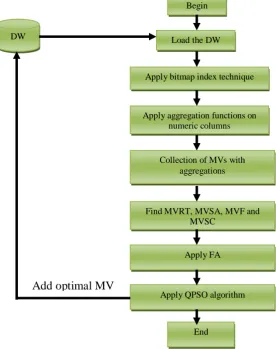
This section introduce the main stages of the proposed work (selection optimal MVs using hybrid technique) as shown in fig. 1.
Fig. 1 The proposed system for selecting optimal MVs using hybrid technique.
Begin
Load the DW
Apply bitmap index technique
Apply aggregation functions on numeric columns
Collection of MVs with aggregations
Find MVRT, MVSA, MVF and MVSC
End
Apply QPSO algorithm Apply FA DW
A. Apply Bitmap Index Technique
The first step in the proposed work is apply the bitmap index on the determined column after computing the column cardinality to decide whether bitmap index is appropriate for this column or not using algorithm in Table 1.
TABLE I
ALGOROTHM TO CALCULATE THE COLUMNS CARDINALITY
Input: selected table from DW.
Output: the cardinality of each column in determined table. Begin
Step (1): select required table from DW.
Step (2): select the determined columns and wait for the answer from the server.
Step (3): the server will calculate the value of cardinality which is the number of distinct groups in the determined column and return it to the end user.
End
B. Apply Aggregation Functions
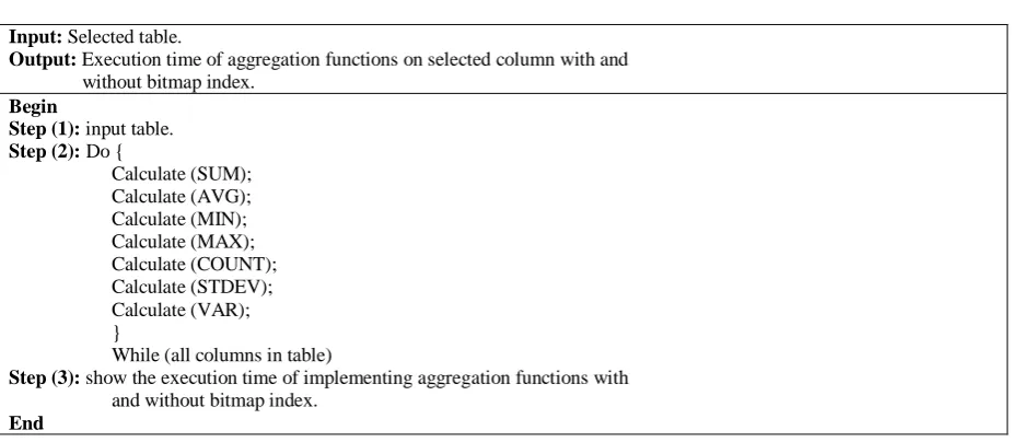
The second step in the proposed work is applying the aggregation functions (AVG, MAX, SUM, MIN, STDEV, VAR and COUNT) on the selected column with two ways (over bitmap index and directly on base tables) using algorithm in Table 2.
TABLE II
ALGORITHM FOR APPLYING AGGREGATION FUNCTIONS
Input: Selected table.
Output: Execution time of aggregation functions on selected column with and without bitmap index.
Begin
Step (1): input table. Step (2): Do {
Calculate (SUM); Calculate (AVG); Calculate (MIN); Calculate (MAX); Calculate (COUNT); Calculate (STDEV); Calculate (VAR); }
While (all columns in table)
Step (3): show the execution time of implementing aggregation functions with and without bitmap index.
End
C. Find Materialized Views Parameters and Selection Costs
After applying aggregation functions in the last step, we have a set of MVs, in this step we will calculate the response time which is the time required for processing this MV, the storage area which is the storage required by current MV and computed by multiplying the MV columns and rows, and the frequency which is how many the current MV requested as MVs information parameters and stored them in MVs information table for calculating the selection cost to each MV in the MVSET using eq. (10)
MVSC= W1* FC+ W2* RTC+ W3* (1- SAC) (10)
Where: W1, W2 and W3 are weights given to FC, RTC and SAC consecutively and their summation is equal to 1. The cost of each parameter has been calculated by dividing the current value of each parameter on the maximum value of this parameter.
TABLE III
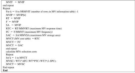
ALGORITHM TO FIND MVS SELECTION COSTS Input: MVs set.
Output: The MVs Selection Costs. Begin
Repeat
MVIT ← MVIP end repeat
Repeat
For k ← 0 to NRMVIT (number of rows in MV information table) -1 MVIP ← MVIP[k]
RT ← MVIP F ← MVIP SA ← MVIP
RTC ← RT/MMVRT (maximum MV response time) FC ← F/MMVF (maximum MV frequency) SAC ← SA/MMVSA (maximum MV storage area) MVCT (MV cost table) ←RTC
MVCT ← FC MVCT ← SAC end repeat
calculate MVs selection costs Repeat
for k ← 1 to MVCT
MVSC= WT1*AFC+WT*PTC+WT3*(1-SPC); MVCT ← MVSC
End repeat End
D. Apply Firefly Algorithm
In this step FA that shown in Table VI has been used to produce optimal initial point to the QPSO algorithm. Firefly algorithm find the brightest one (in this optimization problem the brightest one is the maximum selection cost value), then calculating the distance and attractiveness among the brightest one and other fireflies, finally it reorder the fireflies according the amount of movement of each firefly towards the brightest one until the termination condition is met.
TABLE IV FIREFLY ALGORITHM
Input: two-dimensional matrix of MVs selection costs, maximum number of iterations (M), light absorption coefficient (γ), α.
Output: selection costs reordered based on their movements towards the brightest one. Begin
Step (1): set A=1.
Step (2): begin from the value in the middle, then find the brightest one.
Step (3): compute the distance among the brightest one and other selection costs using eq. (2). Step (4): compute the attractiveness between the brightest one and each selection costs using eq. (1).
Step (5): if the brightness of (xk ) < brightness of (xm ) then firefly (xk ) will move towards firefly (xm ) using eq. (3). Step (6): Ranks MVs selection costs based on their movement.
A=A+1
Step (7): if stopping condition (A>M ) not satisfied then Repeat from step (2)
Else
Take the sorted selection costs. End
E. Apply QPSO Algorithm
The QPSO algorithm which illustrated in Table VI has been used to find optimal MVs which have low response time, low storage area and high frequency for using them to reduce the complex queries response time. At the first step the QPSO algorithm calculates the fitness value of each particle using eq. (11) and eq. (12), and determines the Pbest position. At each iteration, the QPSO algorithm calculates the mean best position of the swarm‟s particle (mbest), as well as evaluates the fitness value of each particle and updates its Pbest and current gbest position before updating its current position until the termination condition is met.
Mean = ∑Ni=1 (Xi)/N (11) Variance= (Xi-mean)2 /N (12) Where:
TABLE V
QUANTUM PARTICLE SWARM OPTIMIZATION ALGORITHM
Input: Search space result from FA (MVs selection costs reordered by FA), r1, r2, r3, parameter α, number of iterations w.
Output: Optimal MV.
Begin
Step(1): set d=1
Step(2): calculate the fitness function for each MV selection cost using eq. (11) and eq. (12). Step(3): determine Pbest position and gbest position.
Step(4): if the fitness of the particle f(x)> fitness of the best particle f(pbest) then go to step(5) else go to step(6). Step(5): f(pbest) = f(x) and pbest = x
F(global) = fitness of the best neighbours of f(x). Step(6): if f(x)> f(global) then
F(global) = f(x) and global = x.
Step(7): update the position of the Pbest particle according eq.(2), calculate the mean best position for new Pbest position Step(8): if (r3<0.5) then
Update the particle position according eq.(8) with (+) sign. Else
Update the particle position according eq.(8) with (-) sign. d=d+1
Step (9): if stopping condition (d>w) not satisfied then Repeat from step(2)
Else
Take optimal MV. End
VIII. THEIMPLEMENTATIONOFTHEPROPOSEDSYSTEM
The sales system data warehouse which built by one of the master‟s project [25] has been taken as a case study. It contains seven dimension tables and one fact table (Suppliers table, Items table, Clients table, Invoices table, Invoices-details table, SuppInvoices table, SuppInvoices-details table and Fact-Sales table).
A. Implementing Bitmap Index
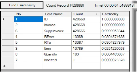
The button “Find Cardinality” in Fig. 2 has been used to calculate the selected column cardinality to decide whether bitmap index is appropriate for this column or not.
Fig. 2 Interface to calculate the columns cardinality.
B. Implementing Aggregation Functions
TABLE VI
ILLUSTRATES THE IMPLEMENTATION OF AGGREGATION FUNCTIONS ON MANY COLUMNS IN VARIOUS TABLES AND THE RESPONSE TIME OF THESE AGGREGATIONS WITH AND WITHOUT BITMAP INDEX TECHNIQUE.
Case NO Filed name
Aggregation Time
Aggregation in relational algebra Function Time using base tables
Time using bitmap index
Case 1 Quatity
Quatity Ꞙsum Quatity (TBL_INVOICE_DETAILS) Sum 00:00:00:078 00:00:00:062
Quatity ꞘAvg Quatity (TBL_INVOICE_DETAILS) Avg 00:00:00:078 00:00:00:078
Quatity ꞘMin Quatity (TBL_INVOICE_DETAILS) Min 00:00:00:093 00:00:00:062 Quatity ꞘMax Quatity (TBL_INVOICE_DETAILS) Max 00:00:00:078 00:00:00:062 Quatity ꞘCount Quatity (TBL_INVOICE_DETAILS) Count 00:00:00:093 00:00:00:046 Quatity ꞘStDev Quatity (TBL_INVOICE_DETAILS) StDev 00:00:00:093 00:00:00:062
Quatity ꞘVar Quatity (TBL_INVOICE_DETAILS) Var 00:00:00:093 00:00:00:062
Case 2 Price
priceꞘsum price (TBL_ITEMS) Sum 00:00:00:031 00:00:00:046
price ꞘAvg price (TBL_ ITEMS) Avg 00:00:00:046 00:00:00:015
price ꞘMin price (TBL_ ITEMS) Min 00:00:00:031 00:00:00:015
price ꞘMax price (TBL_ ITEMS) Max 00:00:00:031 00:00:00:015
price ꞘCount price (TBL_ ITEMS) Count 00:00:00:031 00:00:00:015
price ꞘStDev price (TBL_ ITEMS) StDev 00:00:00:031 00:00:00:031
price ꞘVar price (TBL_ ITEMS) Var 00:00:00:015 00:00:00:031
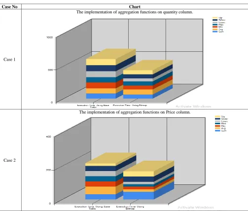
The following Table VII shows the charts of implementing aggregations in Table VI with and without bitmap index (each colour represents a single function).
TABLE VII
SHOWS THE CHARTS OF IMPLEMENTING AGGREGATIONS IN TABLE VI CASE‟S.
Case No Chart
Case 1
The implementation of aggregation functions on quantity column.
Case 2
C. Calculating the MVs Selection costs
In this step the response time, storage area, frequency and them costs have been calculated of each MV as shown in Fig. 3 for using them in calculating the selection cost for each MV in MVSET using eq. (10) as illustrated in Fig. 4.
Fig. 3The costs of MVs parameters.
Fig. 4 The selection costs of each mv in MV set.
D. Implementing Firefly Algorithm
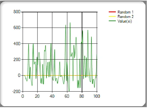
After calculating the MVs selection costs which is two-dimensional matrix contains 625 MVs selection costs as shown in Fig. 5. Firefly algorithm has been applied on this two-dimensional matrix to produce optimal initial point to the QPSO algorithm as shown in Fig. 6.
Fig. 6 The implementaion of FA
E. Implementing QPSO Algorithm
The last step in the proposed work is using QPSO algorithm to find optimal MVs which have low response time, low storage space and high frequency as shown in Fig. 7.
Fig. 7 The implementation of QPSO algorithm.
The location of each particle in the search space resulted by QPSO algorithm is illustrated in fig. 9.
Fig. 9 The position of each particle in QPSO algorithm.
IX.RESULTSDESCUSION
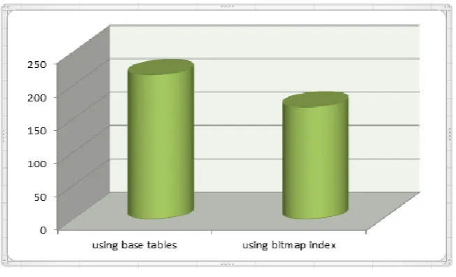
The implementation results proved that bitmap index reduce the MV creation total time. The time difference of applying aggregation functions on one column is sales system DW over base table and over bitmap index is illustrated in Fig. 10, where the total time of applying these functions over bitmap index was found 168 milleseconds, while directly over base tables was found 216 milleseconds.
Fig. 10 The time difference of aggregation functions over bitmap index and over direct access
The optimal MVs resulted by hybrid technique which evaluated based on the three factors (MVRT, MVSA and MVF) to find optimal one which has low response time, low storage area and high frequency have been illustrated in Table VIII.
TABLE VIII
OPTIMAL MVS RESULTED BY HYBRID TECHNIQUE
Iteration NO. Location MVSC SA RT F
60, 197 441 1.2717
74, 166, 168 395 1.3202
76, 78 397 0.2530
79 398 0.6829
80 399 0.9762
33, 101, 183 458 0.7567
160 414 1.1459
29, 95, 177 454 0.7611
The optimal MV which has low response time, storage area as well as high frequency has been found in iteration 61 and the system came back to it again in iterations 67 and 200.
X. CONCLUSIONS
The proposed study introduce an efficient technique to select most beneficial MVs that have low response time and storage area besides high frequency. The implementation results proved that bitmap index achieves good results because it takes less time and storage area in recoupoing results since bitmap indices have the ability of accomplishing processes on index level before recouping the base relations. Also, the hybrid technique (FA and QPSOA) was more efficient in term of optimal MVs selection time since, FA presents optimal initial point to QPSO algorithm.
REFERENCES
[1] D. yao, A. Abulizi, and R. Hou, “An improved algorithm of materialized view selection within the confinement of space,” IEEE Fifth International Conferenc on Big Data and Cloud Computing , 2015. [2] I. Kumar and T. V. V. Kumar, “Materialized View Selection using Discrete Genetic Operators based
Particle Swarm Optimization,” International Conference on Inventive Systems and Control (ICISC), IEEE , 2017.
[3] Mr. P. P. Karde and Dr. V. M. Thakare, “SELECTION OF MATERIALIZED VIEW USING QUERY OPTIMIZATION IN DATABASE MANAGEMENT : AN EFFICIENT METHODOLOGY,” International Journal of Database Management Systems ( IJDMS ), Vol.2 (4), November 2010.
[4] S. Choudhary, and R. Mahajan, “A Design and Implementation of Efficient Algorithm for Materialized View Selection with its Preservation in a Data Warehouse Environment,” International Journal of Science and Research (IJSR), Vol. 4, Issue 11, November 2015.
[5] J. Rajurkar, and T. K. Khan, “Efficient Query Processing and Optimization in SQL using Compressed Bitmap Indexing for Set Predicates,” IEEE Sponsored 9th International Conference on Intelligent Systems and Control (ISCO), 2015.
[6] Ashadevi. B, “Analysis of View Selection Problem in Data Warehousing Environment ,“ International Journal of Engineering and Technology ,Vol.3 (6), pp.447-457, Dec 2011- Jan 2012.
[7] N. Bagheri and M. Sadeghzade, “Using Bat Algorithm for Materialized View Selection in Data Warehouse,” International Journal of Advanced Research in Computer Science and Software Engineering , Vol. 4, Issue 10, October 2014.
[8] M. A. Saleh,” Optimal Selection of Materialized Views and Indexes for Quality Data Warehouse,” A thesis submitted to the Department of Computer Science- College of Computers Science and information technology- University of Anbar In a partial fulfillment of the requirements for the degree of Master in computer science, 2016.
[9] S. U. Khan, W. M. Shah, M. Haris and R. Naseem , “Data Warehouse Enhancement Manipulating Materialized View Hierarchy,” IEEE , 2013.
[10] K. Stockinger and K. Wu, “Bitmap Indices for Data Warehouses,” Computational Research Division Lawrence Berkeley National Laboratory , University of California, 2007.
[11] B. P. S. Chattopadhyay, S. Mitra, R. Chowdhury and Dr. M. De, “Study & Comparison of Indexing Models in Data Warehouses,” International Journal of Software Engineering & Practices, Vol.2, Issue 3, July 2012.
[12] N. Sharma and A. Panwar, “A Comparitive Study of Indexing Techniques in Data Warehouse,” International Journal of Multidisciplinary Sciences and Engineering, Vol. 3(7), July 2012.
[13] M. M. Hamad and M. Abdul-Raheem, “EVALUATION OF BITMAP INDEX USING PROTOTYPE DATA WAREHOUSE,” International Journal of Computers & Technology, Volume 2 (2), April 2012 . [14] Asokan K and A. Kumar R, “Application of Firefly algorithm for solving Strategic bidding to
maximize the Profit of IPPs in Electricity Market with Risk constraints,“ International Journal of Current Engineering and Technology, Vol.4(1), February 2014.
[15] S. K. Pal , C.S Rai and A. P. Singh “Comparative Study of Firefly Algorithm and Particle Swarm Optimization for Noisy Non-Linear Optimization Problems ,“ I.J. Intelligent Systems and Applications, 2012.
[17] Z. T. M. Al-Ta‟i and O. Y. Abd Al-Hameed, “Comparison between PSO and Firefly Algorithms in Fingerprint Authentication”, International Journal of Engineering and Innovative Technology (IJEIT), Volume 3, Issue 1, July 2013.
[18] L. Jing-hui and X. Wen-bo, “The Optimization about PID controller's parameter based on QPSO Algorithm,” IEEE, 10th International Symposium on Distributed Computing and Applications to Business, Engineering and Science, 2011.
[19] R. Li and D. wang, “Clustering Routing Protocol for Wireless Sensor Networks Based on Improved QPSO Algorithm,” IEEE, international conference on advanced mechatronic systems, Xiamen, China, December 6-9, 2017.
[20] M. Chen, J. Ruan, D. Xi, “Micro Grid Scheduling Optimization Based on Quantum Particle Swarm Optimization (QPSO) Algorithm,” IEEE, 2018.
[21] Z. Dongming, X. Kewen, W. Baozhu and G. Jinyong, “An Approach to Mobile IP Routing Based on QPSO Algorithm,” IEEE Pacific-Asia Workshop on Computational Intelligence and Industrial Application, 2008.
[22] I. R. Mohammed, “Image Steganography based on the behavior of Particle Swarm Optimization,” A Thesis Submitted to the Council of the College of Computer - University of Diyala as a Partial Fulfillment of the Requirements for Degree of Master, 2018.
[23] M. Clerc and J. Kennedy, “The Particle Swarm—Explosion, Stability, and Convergence in a Multidimensional Complex Space,” IEEE TRANSACTIONS ON EVOLUTIONARY COMPUTATION, VOL. 6(1), FEBRUARY 2002.
[24] J. Sun, C. Lai and Xiao- Jun, “Particle Swarm Optimization Classical and Quantum Perspective," A Chapman & Hall/CRC Press, 2011.