A Fast Deterministic Algorithm for Side Lobe Level Reduction of Open Loop Coplanar Distributed Antenna Arrays in WSNs

(1)

A Fast Deterministic Algorithm for Side Lobe Level Reduction

of Open Loop Coplanar Distributed Antenna Arrays in WSNs

Haythem H. Abdullah1, Heba S. Dawood2, and Amr H. Hussein2, *

Abstract—Distributed beamforming (DBF) is an eﬃcient technique for reliable communications in wireless sensor networks (WSNs). In DBF based networks, the randomly distributed nodes cooperate to form a randomly distributed antenna array (RAA) which has a main beam directed towards the intended receiver. Due to the nodes randomness, the DBF results in poor pattern characteristics such as high side lobe level (SLL) and pattern asymmetry around the main beam sides. In this paper, a fast deterministic algorithm for SLL reduction of open loop distributed antenna arrays is introduced. Unlike the existing state of the art optimization techniques for SLL reduction, the proposed algorithm provides a fast deterministic solution for energy transmission or the weight of each node without changing its location. Consequently, the exhaustive search burden of the optimization based techniques for the optimum weights is avoided. The simulation results reveal that the proposed algorithm has superior performance to the optimization techniques in terms of execution time, synthesized SLL, and half power beamwidth (HPBW).

1. INTRODUCTION

The traditional antenna arrays consisting of periodic structures such as linear, planar, and circular antenna arrays configurations suffer from scan blindness problem and tight fabrication constraints [1]. Also, the utilization of co-located antennas or traditional arrays in wireless communication systems may lead to significant frequency selective fading, limited transmit power, limited bandwidth, and reduced system capacity. As a promising solution for these critical problems, the distributed antenna networks have been introduced in [2]. In the same context, the distributed Multi-input Multi-output (D-MIMO) has been introduced in [3] for further enhancement of the spectral and energy efficiency of the conventional co-located MIMO (C-MIMO). Wireless Sensor Networks (WSNs) consist of a large number of sensor nodes distributed over a specific area. The nodes are collaborating together for sensing, collecting, and processing information. They have a limited power supply and can’t transmit a signal for a long distance [4]. Distributed beamforming is the key solution for mitigating these problems. In DBF, each sensor node acts as a virtual antenna element to construct a randomly distributed antenna array (RAA). However, the randomness of the distributed nodes creates an array pattern having a high SLL which causes high interference with the unintended receivers located within the same region as well as reducing the received power level at the intended receiver [5, 6]. The interference with the unintended receivers limits the system capacity and increases the bit error rate. As antenna arrays with low side lobe levels are required for efficient and reliable communications, many research works are introduced for SLL reduction of distributed antenna arrays. In [7], a node selection based technique for SLL reduction was introduced. It is mainly based on selecting a combination of nodes from the available set of nodes in the WSN and determines the nodes weights according to their locations.

Received 27 July 2019, Accepted 4 September 2019, Scheduled 21 September 2019

* Corresponding author: Amr Hussein Hussein Abdullah ([email protected], [email protected]).

(2)

However, it depends on the MAC protocol and one-bit feedback from the unintended receiver which is impossible in some cases. In [8], a modiﬁed version of the node selection technique denoted as Bat-Chicken Swarm Optimization (BATCSO) was introduced. It tends to optimize the peak SLL of the array pattern by controlling the nodes transmission energies. A long these lines, a Genetic Algorithm (GA) based technique for SLL minimization was introduced in [9]. It synthesizes the transmission energy of each node without changing the nodes locations. It provides better performance compared to the conventionally distributed beamforming (CDBF). In [10], two Weightless Swarm Algorithm (WSA) and Particle Swarm Optimization (PSO) based techniques were introduced for SLL reduction by adjusting the nodes transmission energy. But, they suﬀer from increased computational complexity. The WSA based technique provided higher SLL reduction than GA and PSO based techniques which consequently improves the signal to noise and interference ratio (SINR) and the capacity of unintended receivers. Along these lines, PSO and Gravitational Search Algorithm (GSA) based SLL reduction techniques were introduced in [11]. They control both transmission energy and transmission phase of each node without any changes in the nodes locations. In [12], a hybrid meta-heuristic optimization algorithm denoted as (PSOGSA-E) which is a combination between the PSO and GSA-Explore was introduced. It suppresses the SLL by optimizing the weight (amplitude and phase) of each node in the RAA. Also, the Non-dominated Sorting GA with selective distance (NSGA-SD) algorithm was introduced in [13]. It provides a bi-objective optimization formulation for the DBF. It controls the weight (amplitude and phase) of each node to minimize the SLL and at the same time maximizes the directivity of the array pattern. But, it is worth pointing to that all the aforementioned SLL reduction techniques which are based on optimization algorithms are time consuming.

There are several applications such as satellite communications, radar systems, and wireless sensor networks where large arrays sizes are very critical to achieve the desired radiation patterns to fulfill the required systems performances. However, large antenna arrays based systems have large computation burden, complex RF front end chains, and high power consumption. To mitigate these problems, adaptive beamforming making the use of sparse characteristics of large antenna arrays based systems is the key solution. In [14], an efficient l0-norm constrained normalized least-mean-square (L0-CNLMS) adaptive beamforming algorithm for controllable sparse antenna arrays was introduced. It is suitable for sparse antenna arrays of different configurations such as standard hexagonal array (SHA) used in satellite communications, rectangular array (RA) used for C-band based radar systems, triangular array (TA) used for P-band based stealth aircraft and satellite detection systems, and irregular arrays (IA) used for S-band communications. Also, it converges faster and utilizes fewer number of antenna elements compared to state of the art sparsity based adaptive beamforming algorithms. However, for non-sparse arrays, its performance is degraded and provides high SLL compared to the conventional non-sparse beamforming algorithms. In the same context, several sparsity based optimization filtering algorithms can be utilized in the SLL reduction as introduced in [15–17]. These algorithms have proved their effectiveness in the well-defined antenna arrays structures such as linear and planar configurations. However, they have to be modified to be applied to randomly distributed antenna arrays. In RAAs, the randomness of nodes distribution may make the separation distances between some of the array nodes to be small enough to maximize the mutual coupling between the neighboring nodes. Several techniques have been introduced to minimize the coupling effect between the antenna arrays elements as in [18] and [19].

(3)

2018. The paper is organized as follows. In Section 2, the system model is introduced. The proposed SLL reduction algorithm is presented in Section 3. The simulation results are illustrated in Section 4. Finally, the paper is concluded in Section 5.

2. SYSTEM MODEL

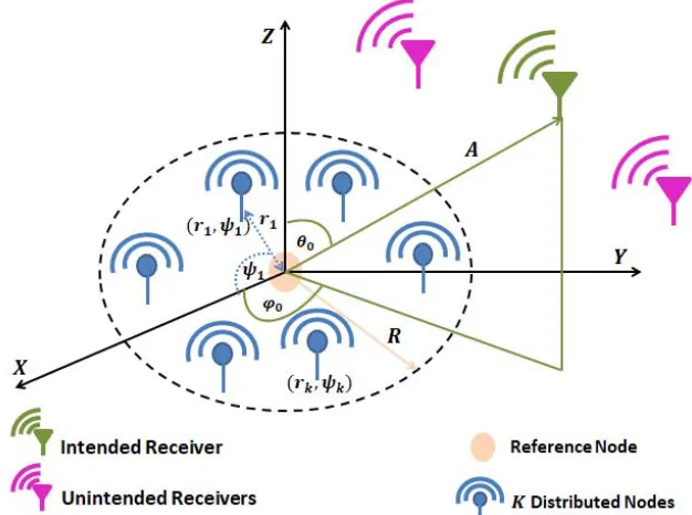
In this section, the geometrical conﬁguration of distributed antenna arrays is introduced. ConsiderK nodes which are distributed over a circular disk of radius R meters. Each node has polar coordinates (rk, ψk) where rk is the distance of the kth node from the central point of the cluster, rk ∈ [0, R],

and ψk is the azimuth angle of the kth node with respect to x-axis, ψk ∈ [−π, π]. It is assumed that

all nodes are isotropic antennas and coplanar with each other. Furthermore, all nodes are perfectly synchronized in phase, time, and frequency. Assume that an intended receiver exists in the proximity of other unintended receivers distributed randomly in space as shown in Fig. 1. The intended receiver has spherical coordinates (A, θ0, ϕ0), whereAis the distance between the intended receiver and the central point of the RAA,θ0the elevation direction,θ0∈[0, π], andϕ0the azimuth direction,ϕ0∈[−π, π] of the intended receiver. The spherical coordinates of theLunintended receivers are (Al, θl, ϕl),l= 1,2, . . . L,

where Al is the distance between the unintended receiver and the central point of the RAA, θl the

elevation direction, θl ∈[0, π], and ϕl the azimuth direction, ϕl ∈[−π, π] of the unintended receivers.

Also, assume that the intended and unintended receivers are located within the same plane as the distributed nodes where θ0 = θl = π₂. Fig. 1 shows the geometrical structure of distributed antenna

array [5].

Figure 1. Geometrical structure of the distributed antenna array.

3. PROPOSED SLL REDUCTION ALGORITHM

In WSNs, to mitigate the high interference with the unintended receivers and increase the received power level at the intended receiver, SLL reduction is the key solution. It signiﬁcantly improves the capacity and the bit error rate performance of the network. In this section, the proposed algorithm for SLL reduction of RAAs is introduced. The steps of the proposed algorithm are presented as follows:

(4)

kth _{node with respect to the center point of the RAA, respectively and} _k _{= 1,}_2,_{3, . . . K}_{. The array}

pattern of the RAA, AF(ϕ) is given by [5]:

AF(ϕ) = 1

K

k=1 wke−j

2π

λrkcos(ϕ−ψ_k) ₍₁₎

wherewk is the transmission weight of thekth node which is given by:

wk =ξkejΨk (2)

where ξk and Ψk are the kth node transmission energy amplitude and initial transmission phase,

respectively. For a uniformly fed array, ξk= 1 and Ψk is determined by [5] as follows:

Ψk =

2π

λrkcos (ϕ0−ψk) (3)

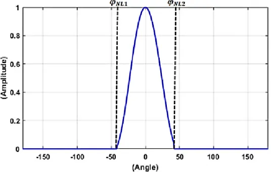
It is required to synthesize an array pattern which has a main beam directed towards the intended receiver with minimum SLL. In this case, the desired array pattern,AFd(ϕ), can be deﬁned as follows:

AFd(ϕ) =

⎧ ⎨ ⎩

0, −π≤ϕ < ϕN L1

AF(ϕ), ϕN L1 ≤ϕ≤ϕN L2

0, ϕN L2 < ϕ≤π

(4)

where ϕN L1 and ϕN L2 are the angles of the ﬁrst two nulls of the ordinary array pattern AF(ϕ). For clariﬁcation, consider the ordinary array pattern forK = 16 elements, R= 1 m, and the main beam is directed at ϕ0 = 0◦. Then, the desired array pattern AFd(ϕ) is plotted as shown in Fig. 2.

Figure 2. The desired array pattern AFd(ϕ) for K = 16 elements, R = 1 m and the main beam

directed at ϕ0 = 0◦.

The synthesized array patternAFsyn(ϕ) should have the same characteristics as the desired array

patternAFd(ϕ) such that:

AFsyn(ϕ) =

1 K

K

k=1 vke−j

2π

λrkcos(ϕ−ψk)∼₌AF_d(ϕ) (5)

wherevkis the synthesized transmission weight of thekthnode which equalsδkejΨk. δkis the synthesized

transmission energy of the kth _{node, while the initial transmission phase Ψ}

k of the kth node remains

ﬁxed as deﬁned in Eq. (3). Substitutingvk in Eq. (5), the synthesized array pattern is rewritten as

AFsyn(ϕ) =

1 K

K

k=1

δkejΨke−j

2π

(5)

To estimate the transmission energy of each node, δk, Eq. (6) is transformed into a matrix form as

follows:

[δ]₁_×_K×[S]_K_×_N = [U]₁_×_N (7)

or for simplicity Eq. (7) is written as:

δS =U (8)

whereN is the number of samples of the desired patternAFd(ϕ). The number of samples is chosen to

be large enough to maintain the pattern smoothness and details. For a given number of samples, N, the sample angles of ϕ∈ [−π, π] can be calculated by:

ϕn =

2nπ

N , n= 1,2,3, . . . N (9)

The elements of [U]₁_×_N vector are the samples of the desired patternAFd(ϕ) at the sample angleϕn

within the range −π ≤ϕ≤π and can be deﬁned as:

[U]₁_×_N = [AFd(ϕ1)AFd(ϕ2). . . AFd(ϕN)] (10)

δ is the (1×K) vector of the synthesized transmission energies of the distributed nodes which is given by

δ= [δ₁δ2. . . δK] (11)

S is aK×N matrix whose elements are given by

Skn=

1

KejΨke−j 2π

λrkcos(ϕn−ψk), k = 1,2, . . . , K and n= 1,2, . . . , N (12)

The synthesized transmission energy vector can be obtained by solving Eq. (8). As S is a non-square matrix, both sides of Eq. (8) are multiplied by the Hermitian transpose of the matrixSwhich is denoted asSH. Then Eq. (8) is written as:

δSSH ₌_USH ₍₁₃₎

LetRSS =SSH which is aK×K square matrix. Then Eq. (13) can be rewritten as:

δRSS =USH (14)

Multiplying both sides of Eq. (14) by the inverse of theRSS matrix, the synthesized transmission energy

vectorcan be calculated by:

δ =USHR_SS−1 (15)

whereR−_SS1 is the inverse of the square matrixRSS.

4. SIMULATION RESULTS

In this section, several simulations are carried out to evaluate and compare the performance of the proposed algorithm with that of the GA based synthesis techniques introduced in [9, 10] and that of the NSGA-SD algorithm introduced in [13]. The GA is utilized to synthesize the antenna array for the maximum SLL reduction by optimizing the transmission energy δ which minimizes the following cost function.

CF(δ) = 20log₁₀max(AF(ϕSL)) AF(ϕM L)

(16)

where AF(ϕSL) is the amplitude of the array pattern at the side lobe angle ϕSL which is deﬁned as

ϕSL ∈ [(−π, ϕN L1)∪(ϕN L2, π)], while AF(ϕM L) is the amplitude of the array pattern at the main

lobe angle ϕM L. Also, the maximum number of iterations (Iga) of the GA is limited to Iga = 100

(6)

4.1. Synthesized Array Pattern Analysis

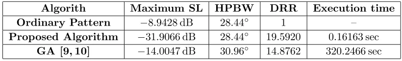
In this section, the synthesized array patterns using the proposed algorithm, GA, and NSGA-SD optimization based techniques are compared with the ordinary array pattern in terms of the maximum SLL, HPBW, execution time, and dynamic range ratio (DRR) which is deﬁned as:

DRR= maximum transmission energy minimum transmission energy =

δmax

δmin

(17)

Four test cases are considered using a small number of nodes distributed over a small circular area of radius R, i.e., (K = 16 and R = 1 m), (K = 8 and R = 1 m), and using a large number of nodes distributed over a moderate area, i.e., (K = 32 and R= 4 m) and (K= 64 and R= 6 m).

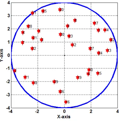
Test case (1): in this case, consider aK = 16 distributed antenna array whose nodes are randomly distributed over a small circular disk area of radius R = 1 m as shown in Fig. 3. The direction of the intended receiver is at the azimuth angle ϕ0 = 0

◦

. The estimated ﬁrst two null angles of the ordinary pattern are ϕN L1 =−34.56◦ and ϕN L2 = 41.04◦. Consequently, the desired array pattern, AFd(ϕ) is

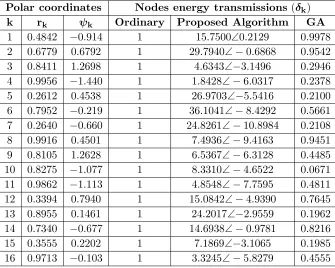
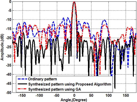
deﬁned according to Eq. (4) and the number of samples is set to N = 1000 samples. The synthesized patterns using the proposed algorithm and the GA based algorithm compared to the ordinary pattern are shown in Fig. 4. The resultant maximum SLL, HPBW, and DRR are listed in Table 1. It is clear that the proposed algorithm provides the lowest SLL and the same HPBW as the ordinary pattern. However, the DRR of the proposed algorithm is slightly greater than that of the GA. Also, it provides about 256.78% reduction in the SLL while the GA provides only 56.60% reduction in the SLL. Using the same number of samplesN = 1000, the estimated execution time of the proposed algorithm is 0.16163 sec which is much lower than the execution time of the GA based algorithm which equals 320.2466 sec. The polar coordinates (rkψk) and nodes energy transmissions (δk) of the synthesized patterns are tabulated

in Table 2.

Figure 3. The nodes distribution forK = 16 and R= 1 m.

Table 1. The resultant maximum SLL, HPBW, DRR, and execution time of the proposed algorithm and the GA compared to the ordinary pattern for K= 16 andR= 1 m.

Algorith Maximum SL HPBW DRR Execution time Ordinary Pattern −8.9428 dB 28.44◦ 1 –

Proposed Algorithm −31.9066 dB 28.44◦ 19.5920 0.16163 sec

(7)

Table 2. The polar coordinates (rk, ψk) and nodes energy transmissions (δk) of the synthesized pattern

forK = 16 and R= 1 m.

Polar coordinates Nodes energy transmissions (δ_k)

k r_k ψ_k Ordinary Proposed Algorithm GA

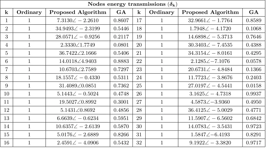
1 0.4842 −0.914 1 15.7500∠0.2129 0.9978 2 0.6779 0.6792 1 29.7940∠−0.6868 0.9542 3 0.8411 1.2698 1 4.6343∠−3.1496 0.2946 4 0.9956 −1.440 1 1.8428∠−6.0317 0.2378 5 0.2612 0.4538 1 26.9703∠−5.5416 0.2100 6 0.7952 −0.219 1 36.1041∠−8.4292 0.5661 7 0.2640 −0.660 1 24.8261∠−10.8984 0.2108 8 0.9916 0.4501 1 7.4936∠−9.4163 0.9451 9 0.8105 1.2628 1 6.5367∠−6.3128 0.4485 10 0.8275 −1.077 1 8.3310∠−4.6522 0.0671 11 0.9862 −1.113 1 4.8548∠−7.7595 0.4811 12 0.3394 0.7940 1 15.0842∠−4.9390 0.7645 13 0.8955 0.1461 1 24.2017∠−2.9559 0.1962 14 0.7340 −0.677 1 14.6938∠−0.9781 0.8216 15 0.3555 0.2202 1 7.1869∠−3.1065 0.1985 16 0.9713 −0.103 1 3.3245∠−5.8279 0.4555

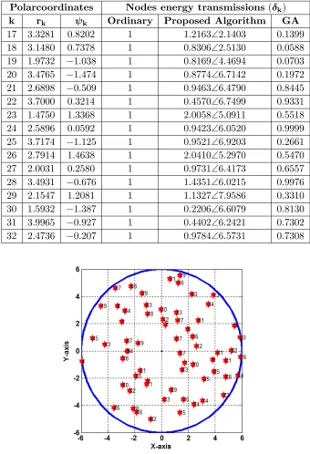
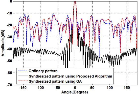
Test case (2): in this case, consider a (K = 32 andR= 4 m) RAA whose main beam is directed at the azimuth angle ϕ0 = 0◦ as shown in Fig. 5. The ﬁrst two null angles of the ordinary pattern are ϕN L1=−8.68◦ andϕN L2 = 8.28◦. Fig. 6 shows the synthesized patterns using the proposed algorithm and the GA compared to the ordinary pattern, and the resultant maximum SLL, HPBW, and DRR are listed in Table 3. The percentages of SLL reduction are 88.36% and 42.98% for the proposed algorithm and the GA based algorithm respectively. The execution time of the proposed algorithm is 0.2523 sec while the execution time of the GA equals 565.0136 sec. Furthermore, the DRR of the proposed algorithm is smaller than that of the GA. The polar coordinates (rk, ψk) and nodes energy

transmissions (δk) of the synthesized patterns are listed in Table 4 and Table 5, respectively.

Proposed Algorithm −16.8359 dB 7.56◦ 17.9752 0.2523 sec GA [6, 7] −12.7795 dB 8.28◦ 187.0206 565.0136 sec

(8)

Figure 4. The synthesized patterns using the proposed algorithm and the GA compared to the ordinary pattern forK = 16 andR= 1 m.

transmissions (δk) of the synthesized patterns are listed in Table 7, Table 8, and Table 9, respectively.

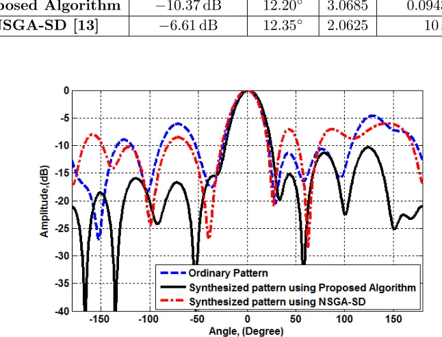
Test case (4): in this case, the proposed algorithm is compared with the NSGA-SD algorithm introduced in [13] for synthesizing a RAA whose parameters are (K = 8 and R = 4 m) as shown in Fig. 9. Fig. 10 shows the synthesized patterns using the proposed algorithm and NSGA-SD compared to the ordinary pattern. The resultant maximum SLL, HPBW, and DRR are listed in Table 10. The simulation results revealed that the proposed algorithm outperforms the NSGA-SD algorithm in terms of maximum SLL reduction and HPBW. It provides SLL reduction of about 123.97% while the NSGA-SD provides a few reduction of about 42.76%. Also, the proposed algorithm provides the same HPBW as the ordinary pattern while the NSGA-SD algorithm provides HPBW which is slightly greater than that of the ordinary pattern. Furthermore, using the same number of samples N = 1000 samples, the proposed algorithm provides a very small execution time of 0.09438 sec which is much lower than the execution time of the NSGA-SD algorithm which equals 10 sec. The polar coordinates (rk, ψk) and

(9)

Polarcoordinates Nodes energy transmissions (δ_k)

1 2.6553 −0.757 1 0.9140∠0.8556 0.3433

2 3.9234 0.3059 1 0.6666∠−0.3410 0.9521 3 2.0722 −0.591 1 0.5477∠0.2746 0.0053 4 3.5536 −0.505 1 0.6914∠−1.1944 0.1701 5 3.1862 0.6389 1 0.5505∠−1.1972 0.0484 6 2.2991 −0.669 1 0.1842∠1.3524 0.0100 7 3.2846 −0.296 1 1.3402∠−0.3347 0.7344 8 2.7649 1.2815 1 1.8963∠1.7440 0.1082 9 2.2200 1.4641 1 3.3109∠−0.6330 0.5389 10 2.1880 −0.544 1 0.4172∠−1.3665 0.5891 11 3.3880 0.5188 1 1.4029∠0.7994 0.4571 12 0.9962 0.9142 1 0.9722∠−2.5973 0.3741 13 3.2684 0.1062 1 1.6215∠0.2036 0.9758 14 3.6165 0.5609 1 1.0629∠0.9961 0.7570 15 2.8659 −0.499 1 0.9242∠1.7201 0.6325 16 3.5685 −1.539 1 0.9499∠−0.9651 0.2144

4.2. Side Lobe Level Analysis

In this section, the resultant SLL is examined under the impact of the variations in the number of nodes, K and the circular area radiusR.

(10)

Polarcoordinates Nodes energy transmissions (δ_k)

17 3.3281 0.8202 1 1.2163∠2.1403 0.1399 18 3.1480 0.7378 1 0.8306∠2.5130 0.0588 19 1.9732 −1.038 1 0.8169∠4.4694 0.0703 20 3.4765 −1.474 1 0.8774∠6.7142 0.1972 21 2.6898 −0.509 1 0.9463∠6.4790 0.8445

22 3.7000 0.3214 1 0.4570∠6.7499 0.9331

23 1.4750 1.3368 1 2.0058∠5.0911 0.5518 24 2.5896 0.0592 1 0.9423∠6.0520 0.9999 25 3.7174 −1.125 1 0.9521∠6.9203 0.2661 26 2.7914 1.4638 1 2.0410∠5.2970 0.5470 27 2.0031 0.2580 1 0.9731∠6.4173 0.6557 28 3.4931 −0.676 1 1.4351∠6.0215 0.9976 29 2.1547 1.2081 1 1.1327∠7.9586 0.3310 30 1.5932 −1.387 1 0.2206∠6.6079 0.8130 31 3.9965 −0.927 1 0.4402∠6.2421 0.7302 32 2.4736 −0.207 1 0.9784∠6.5731 0.7308

GA, and the ordinary pattern are shown in Fig. 11. The simulation results revealed that the proposed algorithm outperforms the GA technique as it provides maximum SLL range (from −31.9066 dB to −40.3119 dB) when K changes from (K = 16 to K = 80). However, the ordinary pattern and the GA provide maximum SLL range (from −8.9428 dB to −14.7544 dB) and (from −14.0047 dB to −32.3507 dB), respectively.

(11)

GA [9, 10] −12.8419 dB 5.5◦ 62.8482 1721.023 sec

(12)

the entire range of disk radius. It provides maximum SLL range ( from −31.9066 dB to −7.8920 dB) when the disk radius R changes from (R = 1 m to 10 m). However, the ordinary pattern and the GA provide maximum SLL ranges (from−8.9428 dB to−3.9208 dB) and (from−14.0047 dB to−5.5796 dB) respectively.

Table 7. The polar coordinates (rk, ψk) for K = 64 andR = 6 m.

Polarcoordinates

k r_k ψ_k k r_k ψ_k k r_k ψ_k k r_k ψ_k

1 1.9157 −0.471 17 2.5249 1.0758 33 3.5861 −1.521 49 1.8737 −0.303 2 3.6516 −0.621 18 4.7466 1.1031 34 4.8725 0.7798 50 3.8408 0.7141 3 5.7384 0.3249 19 5.6172 −0.6290 35 3.7670 −0.584 51 2.1731 0.7369 4 5.9970 0.1321 20 2.5328 −0.405 36 2.5348 0.4253 52 5.2119 0.0044 5 2.4775 1.1248 21 4.8209 −0.149 37 1.3981 0.6896 53 3.5400 −1.236 6 2.4928 0.6844 22 5.6417 −0.614 38 2.9827 0.1857 54 4.0240 −0.822 7 1.9263 1.4323 23 3.0031 1.1940 39 5.6978 1.3289 55 2.6788 0.7561 8 4.6713 −0.779 24 4.5939 −1.023 40 5.9471 0.1632 56 5.1492 1.3315 9 3.8507 −0.167 25 4.1866 −0.370 41 4.1747 −0.036 57 2.7058 0.2669 10 3.0345 −1.556 26 5.4961 0.8670 42 2.2828 1.5371 58 5.2587 −1.116 11 2.6946 1.1376 27 1.3639 −0.123 43 4.2919 −0.111 59 2.9472 −1.325 12 2.5994 0.1341 28 5.1596 −0.379 44 5.9806 −0.305 60 4.7005 −1.077 13 5.6406 0.8122 29 4.4680 −1.232 45 5.2395 −0.178 61 3.5281 0.6887 14 4.7677 −0.879 30 3.9320 −1.145 46 5.8972 −0.078 62 5.1005 1.4072 15 4.7336 −1.277 31 5.2981 1.4547 47 5.7858 −0.924 63 2.0543 −0.737 16 4.8680 1.1787 32 3.7789 0.8876 48 2.9178 −1.199 64 2.5512 0.0031

Table 8. The nodes energy transmissions (δk) of the synthesized pattern forK = 64 and R= 6 m.

Nodes energy transmissions(δk)

(13)

Table 9. The nodes energy transmissions (δk) of the synthesized pattern forK = 64 and R= 6 m.

Nodes energy transmissions(δk)

k Ordinary Proposed Algorithm GA k Ordinary Proposed Algorithm GA 33 1 2.3079∠−6.8117 0.1726 49 1 3.9142∠−11.3588 0.7557 34 1 16.5709∠−7.0848 0.9876 50 1 20.7471∠−12.0369 0.9212 35 1 36.6102∠−6.6202 0.7685 51 1 28.2178∠−10.1590 0.8000 36 1 28.5454∠−9.2038 0.7136 52 1 8.9211∠−12.0014 0.8768 37 1 25.1721∠−5.8573 0.9249 53 1 11.8328∠−11.4923 0.3159 38 1 12.5651∠−6.6190 0.9840 54 1 5.1548∠−11.3130 0.2939 39 1 1.5942∠−7.0245 0.2941 55 1 20.9906∠−12.3521 0.6820 40 1 20.2395∠−6.8799 0.9397 56 1 2.2180∠−12.3755 0.0664 41 1 24.6302∠−9.6349 0.3558 57 1 5.0911∠−15.6113 0.2043 42 1 4.0354∠−7.8365 0.4616 58 1 4.2611∠−12.8152 0.2024 43 1 16.3730∠−9.4768 0.0829 59 1 26.4804∠−14.6527 0.6462 44 1 12.6796∠−9.5369 0.4293 60 1 3.0665∠−14.3484 0.1310 45 1 29.0337∠−10.6186 0.4842 61 1 29.6211∠−14.6274 0.0178 46 1 3.7763∠−9.7732 0.5034 62 1 2.4838∠−16.8718 0.6771 47 1 3.0559∠−11.5927 0.5997 63 1 26.0455∠−18.5841 0.8941 48 1 5.4749∠−14.6929 0.7557 64 1 11.4999∠−18.4030 0.7483

Table 10. The resultant maximum SLL, HPBW, and DRR of the proposed algorithm and the NSGA-SD compared to the ordinary pattern forK = 8 andR = 4 m.

NSGA-SD [13] −6.61 dB 12.35◦ 2.0625 10 sec

(14)

Table 11. The polar coordinates (rk, ψk) and nodes transmission weights (vk) of the synthesized

pattern forK = 8 and R= 4 m.

Polar coordinates Nodes transmissions weight (v_k)

k r_k ψ_k Ordinary Proposed Algorithm NSGA−SD

1 0 0 1∠0.12 1.2661∠−0.6484 0.53∠0.18 2 3.2755 0.5855 1∠1.31 0.5252∠0.5315 0.94∠1.10 3 3.1219 −0.343 1∠−0.69 0.4938∠−1.158 0.31∠−1.12 4 0.6868 0.8369 1∠0.10 1.5151∠0.8978 0.19∠0.05 5 2.8898 1.2064 1∠−1.73 1.1818∠−1.2798 0.76∠−1.03 6 2.7509 −1.545 1∠2.19 0.6784∠2.2068 0.56∠2.05 7 1.7605 0.0227 1∠−0.12 0.8861∠0.3869 0.97∠0.01 8 2.5911 1.4158 1∠0.04 1.1477∠−0.5825 0.72∠0.16

Figure 11. The maximum SLL versusK forR= 1 m.

(15)

5. CONCLUSION

In this paper, a fast deterministic distributed beamforming algorithm is proposed for maximum SLL reduction of RAAs in wireless sensor networks. It controls the energy transmission δ_k or transmission weight (v_k) of each node without altering the nodes locations. The simulation results verify the feasibility and eﬀectiveness of the proposed algorithm compared to the recent state of the art GA and NSGA-SD optimization based techniques. It provides the highest SLL reduction while maintaining the same HPBW as the ordinary pattern. Furthermore, it is not time consuming which makes it suitable for adaptive beamforming of distributed random antenna arrays.

REFERENCES

1. Bhattacharyya, K., Phased Array Antennas: Floquet Analysis, Synthesis, BFNs and Active Array Systems, John Wiley & Sons, 2006.

2. Adachi, F., W. Peng, T. Obara, T. Yamamoto, R. Matsukawa, and S. Nakada, “Distributed antenna network for gigabit wireless access,” International Journal of Electronics and Communications (AE ¨U), Vol. 66, No. 8, 605–612, 2012.

3. Jung, S. Y. and B. W. Kim, “Near-optimal low-complexity antenna selection scheme for energy-eﬃcient correlated distributed MIMO systems,” International Journal of Electronics and Communications (AE ¨U), Vol. 69, No. 7, 1039–1046, 2015.

4. Valenzuela-Valdes, J., F. Luna, R. Luque-Baena, and P. Padilla, “Saving energy in WSNs with beamforming,” IEEE, International Conference on Cloud Networking, 255–260, 2014.

5. Ochiai, H., P. Mitran, H. V. Poor, and V. Tarokh, “Collaborative beamforming for distributed wireless ad hoc sensor networks,”IEEE Transactions on Signal Processing, Vol. 53, No. 11, 4110– 4124, 2005.

6. Jayaprakasam, S., S. K. A. Rahim, and C. Y. Leow, “Distributed and collaborative beamforming in wireless sensor networks: Classiﬁcations, trends, and research directions,” IEEE Communications Surveys& Tutorials, Vol. 19, No. 4, 2092–2116, 2017.

7. Ahmed, M. F. and S. A. Vorobyov, “Sidelobe control in collaborative beamforming via node selection,” IEEE Transactions on Signal Processing, Vol. 58, No. 12, 6168–6180, 2010.

8. Liang, S., T. Feng, G. Sun, J. Zhang, and H. Zhang, “Transmission power optimization for reducing sidelobe via bat-chicken swarm optimization in distributed collaborative beamforming,” IEEE International Conference on Computer and Communications (ICCC), 2164–2168, 2016.

9. Jayaprakasam, S., S. Rahim, L. C. Yen, and K. Ramanathan, “Genetic algorithm based weight optimization for minimizing sidelobes in distributed random array beamforming,” IEEE International Conference on Parallel and Distributed Systems, 623–627, 2013.

10. Jayaprakasam, S., S. K. A. Rahim, C. Y. Leow, and T. O. Ting, “Sidelobe reduction and capacity improvement of open-loop collaborative beamforming in wireless sensor networks,” PloS one, Vol. 12, No. 5, 1–33, 2017.

11. Jayaprakasam, S., S. K. A. Rahim, C. Y. Leow, and M. F. M. Yusof, ‘Beampatten optimization in distributed beamforming using multiobjective and metaheuristic method,”IEEE Symposium on Wireless Technology and Applications (ISWTA), 86–91, 2014.

12. Jayaprakasam, S., S. Rahim, and C. Y. Leow, “PSOGSA-explore: A new hybrid metaheuristic approach for beampattern optimization in collaborative beamforming,” Applied Soft Computing, Vol. 30, 229–237, 2015.

13. Jayaprakasam, S., S. K. A. Rahim, C. Y. Leow, T. O. Ting, and A. A. Eteng, “Multiobjective beampattern optimization in collaborative beamforming via NSGA-II with selective distance,” IEEE Transactions on Antennas and Propagation, Vol. 65, No. 5, 2348–2357, 2017.

14. Shi, W., Y. Li, L. Zhao, and X. Liu, “Controllable sparse antenna array for adaptive beamforming,” IEEE Access, Vol. 7, 6412–6423, 2019.

(16)

16. Li, Y., Y. Wang, and T. Jiang, “Sparse-aware set-membership NLMS algorithms and their application for sparse channel estimation and echo cancelation,” AEU — International Journal of Electronics and Communications, Vol. 70, No. 7, 895–902, 2016.

17. Li, Y., Z. Jiang, W. Shi, X. Han, and B. Chen, “Blocked maximum correntropy criterion algorithm for cluster-sparse system identiﬁcations,” IEEE Transactions on Circuits and Systems II: Express Briefs, 2109.

18. Yu, K., Y. Li, and X. Liu, “Mutual coupling reduction of a MIMO antenna array using 3-D novel meta-material structures,”Applied Computational Electromagnetics Society Journal, Vol. 33, No. 7, 758–763, 2018.