Embedded Extended Visual Cryptography Schemes

Embedded Extended Visual Cryptography Schemes Feng Liu1 _{and ChuanKun Wu}1

1_{The State Key Laboratory of Information Security}

Institute of Software, Chinese Academy of Sciences, Beijing 100190 China Email: {liufeng, ckwu}@is.iscas.ac.cn

Homepage: http://iscas.ac.cn/ liufeng

Abstract

Visual cryptography scheme (VCS) is a kind of secret sharing scheme which allows the encoding of a secret image into 𝑛 shares that distributed to 𝑛 participants. The beauty of such scheme is that a set of qualified participants is able to recover the secret image without any cryptographic knowledge and computation devices. Extended visual cryptography scheme (EVCS) is a kind of VCS which consists of meaningful shares (compared to the random shares of traditional VCS). In this paper, we propose a construction of EVCS which is realized by embedding random shares into meaningful covering shares, and we call it the embedded ex-tended visual cryptography scheme (embedded EVCS). Experimental results compare some of the well-known EVCS’s proposed in recent years systematically, and show that the proposed embedded EVCS has competitive visual quality compared with many of the well-known EVCS’s in the literature. Besides, it has many specific advantages against these well-known EVCS’s respectively.

Keywords: Secret sharing, Embedded extended visual cryptography scheme

1 Introduction

Many other applications of VCS, other than its original objective (i.e. sharing secret image), have been found, for example, authentication and identification [4], watermarking [5] and transmitting passwords [6] etc..

Figure 1: An example of traditional (2,2)-VCS with image size 128×128.

The associated secret sharing problem and its physical properties such as contrast, pixel expan-sion and color were extensively studied by researchers worldwide. For example, Naor et al. [3] and Blundo et al. [7] showed constructions of threshold VCS with perfect reconstruction of the black pixels. Ateniese et al. [8] gave constructions of VCS for the general access structure. Krishna et al., Luo et al., Hou et al. and Liu et al. considered color visual cryptography schemes [9–12]. Shyu et al. proposed a scheme which can share multiple secret images [13]. Furthermore, Eisen et al. proposed a construction of threshold VCS for specified whiteness levels of the recovered pixels [14]. The term of extended visual cryptography scheme (EVCS) was first introduced by Naor et al. in [3], where a simple example of (2,2)-EVCS was presented. In this paper, when we refer to a corresponding VCS of an EVCS, we mean a traditional VCS that have the same access structure with the EVCS. Generally, an EVCS takes a secret image and 𝑛 original share images as inputs, and outputs𝑛shares that satisfy the following three conditions: (1) Any qualified subset of shares can recover the secret image; (2) Any forbidden subset of shares cannot obtain any information of the secret image other than the size of the secret image; (3) All the shares are meaningful images. Examples of EVCS can be found in the experimental results of this paper, such as Figure 4, 5 and 6.

EVCS can also be treated as a technique of steganography. One scenario of the applications of EVCS is to avoid the custom inspections, because the shares of EVCS are meaningful images, hence there are fewer chances for the shares to be suspected and detected.

the share images. Recently, Wang et al. proposed three EVCS’s by using error diffusion halftoning technique [23] to obtain nice looking shares. Their first EVCS also made use of complementary shares to cover the visual information of the shares as the way proposed in [20]. Their second EVCS imported auxiliary black pixels to cover the visual information of the shares. In such a way, each qualified participants did not necessarily require a pair of complementary share images. Their third EVCS modified the halftoned share images and imported extra black pixels to cover the visual information of the shares.

However, the limitations of these EVCS’s mentioned above are obvious. The first limitation is that the pixel expansion is large (Formal definitions of pixel expansion will be given in Definition 1 of Section 2.1). For example, the pixel expansion of the EVCS in [16] is𝑚+𝑞, where𝑚is the pixel expansion of the secret image and𝑞is the chromatic number of a hyper-graph, in any case the value of 𝑞 satisfies 𝑞≥2. The construction in [15] has the pixel expansion∑𝑛_𝑞=12𝑞−1_{𝑏𝑞, where 𝑏𝑞 is the} number of elements of𝑆 which contains exactly𝑞 elements, and𝑆is the set of the qualified subsets. For example, for a (3,3)-EVCS, the pixel expansion will be 13 (see the last example of Section 7 in [15]). The pixel expansion of the (𝑘, 𝑛)-EVCS in [17] is𝑚+𝑚0 where𝑚0 ≥ ⌈𝑛/(𝑘−1)⌉. The second limitation is the bad visual quality of both the shares and the recovered secret images; this is confirmed by the comparisons in [20]. Unfortunately, the EVCS in [20] has other limitations, first it is computation expensive, second, the void and cluster algorithm makes the positions of the secret pixels dependent on the content of the share images and hence decrease the visual quality of the recovered secret image, third and most importantly, a pair of complementary images are required for each qualified subset and the participants are required to take more than one shares for some access structures, which will inevitably cause the attentions of the watchdogs at the custom and increase the participants’ burden. The same problems also exist in the first method proposed by Wang et al. [23]. For Wang et al.’s second method, each qualified subset does not require complementary images anymore; however, this method is only for threshold access structure, and the auxiliary black pixels of their EVCS also darkened the shares. In fact, the way of generating auxiliary black pixels of this method can be viewed as a special case of our approach in Section 4 of this paper. For Wang et al.’s third method, the halftoned share images are modified and extra black pixels are imported to cover the visual information of the shares. The limitation of this method is that, the visual effect of each share will be affected by the content of other shares, and the content of the input original share images should be chosen in a selected way.

Tsai et al.’s EVCS [19] is simple, but it may not satisfy the contrast condition of anymore. And the recovered secret image contains the mixture of the visual information of share images. Consider the essence of mixing grey-level pixels; the secret information may be hard to be recognized by human eyes.

dynamic range. (Explicit discussions on the security of the EVCS in [18] can be found in Section 4.2 of [18]).

The rest of this paper is organized as follows: Section 2 gives some preliminary results about VCS and the halftoning technique. In Section 3, we introduce the formal definition of embedded EVCS, and give the main idea about our construction. In Section 4, we give two methods to generate the covering shares. In Section 5, we embed the traditional VCS into the covering shares and discuss the bounds of our scheme. In Section 6, we propose a method to further reduce the black ratio, which enhances the visual quality of the shares. In Section 7, we give some experimental results and comparisons. At last, in Section 8, we conclude the paper.

2 Preliminaries

In this section, we give some definitions about VCS and some preliminary results about the halftoning technique by using the dithering matrix.

2.1 Definitions of traditional VCS

Suppose all the participants of a secret sharing scheme is 𝒱 = {0,1, . . . , 𝑛−1}. The spec-ifications of all qualified and forbidden subsets of participants constitute an access structure (Γ𝑄𝑢𝑎𝑙,Γ𝐹 𝑜𝑟𝑏), where Γ𝑄𝑢𝑎𝑙 is the superset of qualified subsets, and Γ𝐹 𝑜𝑟𝑏 is the superset of

for-bidden subsets, and Γ𝑄𝑢𝑎𝑙∩Γ𝐹 𝑜𝑟𝑏 =∅. In this paper we only consider the access structure with

Γ𝑄𝑢𝑎𝑙∪Γ𝐹 𝑜𝑟𝑏 = 2𝒱. The superset Γ𝑄𝑢𝑎𝑙 is monotone because if part of the participants in a set 𝐵(∈ Γ𝑄𝑢𝑎𝑙) can recover the shared secret, then it is obvious that all the participants in 𝐵 can

recover the shared secret as well. Let

Γ𝑚 ={𝐴∈Γ𝑄𝑢𝑎𝑙:∀𝐵 ⊈𝐴⇒𝐵 /∈Γ𝑄𝑢𝑎𝑙} and Γ𝑀 ={𝐴∈Γ𝐹 𝑜𝑟𝑏 :∀𝐵 ⊋𝐴⇒𝐵 /∈Γ𝐹 𝑜𝑟𝑏}

Then Γ𝑚 is calledthe minimal qualified access structure, Γ𝑀 is calledthe maximal forbidden access

structure. For the superset of subsets 𝒞 ⊆2𝒱_{, define𝑐𝑙(𝒞) ={𝐵 ⊆ 𝒱 :∃𝐴∈ 𝒞𝑠𝑡. 𝐵 ⊇𝐴}. We call}

𝑐𝑙(𝒞) the closure of 𝒞. Since Γ𝑄𝑢𝑎𝑙 is monotone, then 𝑐𝑙(Γ𝑚) = Γ𝑄𝑢𝑎𝑙. From the above discussion

it is known that the qualified access structure Γ𝑄𝑢𝑎𝑙 and the minimal qualified access structure Γ𝑚

are determined by each other, so when we discuss the qualified access structure, we only need to give discussions on the minimal qualified access structure in the rest of this paper.

The threshold access structure is a special case of the general access structure. More specifically, a threshold (𝑘, 𝑛) access structure is a general access structure satisfies the following

Γ𝑄𝑢𝑎𝑙={𝐵⊆ 𝒱 :∣𝐵∣ ≥𝑘}and Γ𝐹 𝑜𝑟𝑏={𝐵⊆ 𝒱 :∣𝐵∣ ≤𝑘−1}

and

Take a (2,3) access structure as an example. We have Γ𝑄𝑢𝑎𝑙={{1,2},{2,3},{1,3},{1,2,3}},

Γ𝐹 𝑜𝑟𝑏 ={{},{1},{2},{3}}, Γ𝑚={{1,2},{2,3},{1,3}} and Γ𝑀 ={{1},{2},{3}}.

In this paper, we will focus on black and white secret image only, where the white pixel is denoted by 0 and the black pixel is denoted by 1. Generally, a VCS consists of a pair of collections of matrices (𝐶0, 𝐶1). The matrices in the collections (𝐶0, 𝐶1) are called share matrices, where each share matrix consists of 𝑛×𝑚 sub-pixels. However, many studies make use of basis matrices to simplify their discussions (see examples in [7, 8, 14, 16, 17, 24]). Now we give the formal definition of the basis matrix VCS as follows.

Definition 1 (Basis Matrix VCS [8]) Let (Γ𝑄𝑢𝑎𝑙,Γ𝐹 𝑜𝑟𝑏) be an access structure on a set of 𝑛

participants. The boolean𝑛×𝑚matrices𝑀0 _and𝑀1_{are the basis matrices of a visual cryptography} scheme if there exist values {ℎ𝑋 : 𝑓𝑜𝑟 𝑋∈Γ𝑄𝑢𝑎𝑙} and𝛼(>0)satisfying:

1. (Contrast) If𝑋={𝑖1, 𝑖2,⋅ ⋅ ⋅ , 𝑖𝑝} ∈Γ𝑄𝑢𝑎𝑙, then the ORof rows𝑖1, 𝑖2,⋅ ⋅ ⋅, 𝑖𝑝 of𝑀0 is a vector 𝑣 that satisfies 𝑤(𝑣)≤(ℎ𝑋 −𝛼𝑚), whereas, for𝑀1, we have that 𝑤(𝑣)≥ℎ𝑋.

2. (Security) If𝐹 ={𝑖1, 𝑖2,⋅ ⋅ ⋅, 𝑖𝑝} ∈Γ𝐹 𝑜𝑟𝑏, then the𝑝×𝑚 matrices obtained by restricting𝑀0

and 𝑀1 _{to rows𝑖}

1, 𝑖2,⋅ ⋅ ⋅ , 𝑖𝑝 are equal up to a column permutation.

In the above definition,

∙ 𝑤(𝑣) is the hamming weight of a vector 𝑣.

∙ 𝑚 is called the pixel expansion of the traditional VCS. Besides, in this paper, we also define the secret image pixel expansion as the pixel expansion of the recovered secret image over the original secret image, and we define the share pixel expansion as the pixel expansion of the final output shares over the original share images.

∙ 𝛼 is called the contrast of the recovered secret image.

∙ ℎ𝑋 is called the threshold of a qualified subset𝑋.

2.2 Halftoning technique by using dithering matrix

One of the main drawbacks of the VCS’s proposed in [3, 7, 8, 16] is that, they cannot deal with the grey-scale image. MacPherson [24] proposed a VCS to deal with the grey-scale image, however, it has large pixel expansion 𝑐×𝑚, where𝑐is the number of the grey-levels and 𝑚 is the pixel expansion of the corresponding black and white VCS. In order to deal with the grey-scale image, the halftoning technique was introduced into the visual cryptography [11, 18, 25–27]. The halftoning technique (or dithering technique) is used to convert the grey-scale image into the binary image. This technique has been extensively used in printing applications which has been proved to be very effective. Once we have the binary image, the VCS proposed in [3, 7, 8, 16] can be applied directly. However, the concomitant loss in quality is unavoidable in this case.

Many kinds of halftone algorithms have been proposed in the literature. In this paper, we make use of the patterning dithering [28]. The patterning dithering makes use of a certain percentage of black and white pixels, often called patterns, to achieve a sense of grey scale in the overall point of view. The pattern consists of black and white pixels, where different percentage of the black pixels stands for the different greynesses. The halftoning process is to map the grey scale pixels from the original image into the patterns with certain percentage of black pixels. The halftoned image is a binary image. However, in order to store the binary images one needs a large amount of memory. A more efficient way is by using the dithering matrix. The dithering matrix is a 𝑐×𝑑

integer matrix, denoted as 𝐷. The entries, denoted as 𝐷𝑖,𝑗 for 0≤𝑖≤𝑐−1 and 0≤𝑗 ≤𝑑−1,

of the dithering matrix are integers between 0 and 𝑐𝑑−1, which stand for the grey-levels in the dithering matrix. Denote 𝑔 ∈ {0,⋅ ⋅ ⋅, 𝑐𝑑} as the grey-levels of a pixel in the original image. The halftoning process is formally described in Algorithm 1.

Generally, for an input image𝐼 of size 𝑝×𝑞, the halftoning process runs on each pixel in𝐼 as follows.

Algorithm 1 The halftoning process for each pixel in 𝐼:

Input: The 𝑐×𝑑dithering matrix 𝐷 and a pixel𝑥 with grey-level 𝑔 in input image𝐼

Output: The halftoned pattern at the position of the pixel 𝑥

For𝑖= 0to𝑐−1 do

For𝑗 = 0 to𝑑−1 do

If 𝑔≤𝐷𝑖𝑗 then print a black pixel at position (i,j);

Else print a white pixel at position (i,j);

To describe the halftoning process clearer, take the dithering matrix with 10 (= 3×3 + 1) grey-levels as an example, where the grey-levels of the original image range from 0 to 9.

𝐷0=

7 0 5 2 4 6 3 8 1

Matrix 1: Dithering matrix with 10 grey-levels𝐷0.

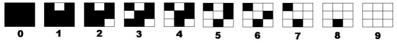
In Algorithm 1, the halftoning process causes the 𝑐𝑑pixel expansion on the input image. We call it the halftone pixel expansion. In the rest of the paper, we denote 𝑠 as the halftone pixel expansion, i.e. 𝑠=𝑐𝑑. Take the above dithering matrix𝐷0 as an example, the halftoned patterns of the grey-levels 0,⋅ ⋅ ⋅ ,9 are shown in Figure 2.

Figure 2: The halftoned patterns of the dithering matrix𝐷0 of the grey-levels 0,⋅ ⋅ ⋅ ,9.

3 A sketch and the main idea of the proposed embedded EVCS

In this section, we will give an overview of our construction. First we introduce the formal definition of embedded EVCS.

Definition 2 (embedded EVCS) Denote𝑀0_and𝑀1 _{as the basis matrices of a traditional VCS} with access structure (Γ𝑄𝑢𝑎𝑙,Γ𝐹 𝑜𝑟𝑏) and pixel expansion 𝑚. In order to encode a secret image 𝐼,

the dealer takes 𝑛 grey-scale original share images as inputs, and converts them into 𝑛 covering shares which are divided into blocks of 𝑡sub-pixels (𝑡≥𝑚). By embedding the rows of 𝑀0 _and𝑀1 (after randomly permuting their columns) into the blocks, the embedded EVCS outputs 𝑛 shares

𝑒0,⋅ ⋅ ⋅ , 𝑒𝑛−1, and there exist values {ℎ𝑋 : 𝑓𝑜𝑟 𝑋∈Γ𝑄𝑢𝑎𝑙}, 𝛼 and 𝜌 satisfying:

1. The stacking result of each block of a qualified subset of shares can recover a secret pixel. More precisely, if 𝑋 = {𝑖1,⋅ ⋅ ⋅, 𝑖𝑝} ∈ Γ𝑄𝑢𝑎𝑙, denote 𝐵𝑖1,⋅ ⋅ ⋅, 𝐵𝑖𝑝 as the blocks at the same

position of the shares 𝑒𝑖1,⋅ ⋅ ⋅ , 𝑒𝑖𝑝, then for a white secret pixel, the OR of 𝐵𝑖1,⋅ ⋅ ⋅ , 𝐵𝑖𝑝 is a

vector𝑣 that satisfies𝑤(𝑣)≤ℎ𝑋−𝛼𝑡, and that for a black secret pixel, it satisfies𝑤(𝑣)≥ℎ𝑋.

2. Part of the information of the original share images is preserved in the shares. Define 𝜌 = (𝑡−𝑚)/𝑡 be the ratio of the information of the original share images that preserved in the shares, and it satisfies 𝜌 >0.

meaningful in the sense that parts of the information of the original share images are preserved. The value 𝜌 reflects the ratio of the information of the original share images that preserved in the shares. Explicitly, the value of𝜌 is between 0 and 1, where𝜌= 0 means that no information of the original share images can be observed, and 𝜌 = 1 means that all the information of the original share images can be observed. Generally, when𝜌 >0, the shares can be considered as meaningful. The larger the value of𝜌is the better visual quality the shares will have. At last, Definition 2 does not have the security condition. The secret image is, in fact, encrypted by the corresponding VCS, and then we embed its shares into the covering shares. Hence, the security of the embedded EVCS is guaranteed by the security of the corresponding VCS, i.e. the security condition of Definition 1. Furthermore, we need to point out that, in [16], Ateniese et al. proved the optimality of their scheme under their definition of EVCS. Under the definition of Ateniese et al., all the information of the original share images is preserved in the shares. However, as the second condition of the above Definition 2 indicates, only parts of the information of the original share images are preserved in the shares, i.e. Definition 2 is a relaxed model of the EVCS model proposed in [16]. Hence our scheme can have smaller pixel expansion by sacrificing part of the information of the original share images. We claim that our definition is reasonable, because the information of the original share images is not as important as that of the secret image for the participants. Besides, experimental results of this paper show that preserving all the information of original share images does not imply better visual quality of the final output shares.

The idea of our embedded EVCS contains two main steps: (1) Generate 𝑛 covering shares, denoted as 𝑠0, 𝑠1,⋅ ⋅ ⋅, 𝑠𝑛−1; (2) Generate the embedded shares by embedding the corresponding VCS into the 𝑛covering shares, denoted as 𝑒0, 𝑒1,⋅ ⋅ ⋅, 𝑒𝑛−1.

In step 1, we generate the covering shares for an access structure Γ𝑚. We take 𝑛 grey-scale

original share images, denoted as 𝐼0, 𝐼1,⋅ ⋅ ⋅, 𝐼𝑛−1, as the inputs, and output 𝑛binary meaningful shares 𝑠0, 𝑠1,⋅ ⋅ ⋅ , 𝑠𝑛−1, where the stacking results of the qualified shares are all black images, i.e.

shares covers all the information of the original share images. The detailed information about the embedding process will be introduced in Section 5.

4 Generating the covering shares by using the dithering matrices

In this section, we propose a method to construct the covering shares𝑠0, 𝑠1,⋅ ⋅ ⋅, 𝑠𝑛−1 by using the𝑛 input original share images𝐼0, 𝐼1,⋅ ⋅ ⋅ , 𝐼𝑛−1.

Let𝐷0 be the dithering matrix in Example 1. Suppose the grey-levels of all the pixels in the image 𝐼0 are smaller than 4, then the positions corresponding to 𝐷000 ,𝐷002, 𝐷011, 𝐷012 and 𝐷021 of all the pixels in the image 𝐼₀′ are always black after being halftoned by 𝐷0, where𝐷0

𝑖𝑗 is the entry

in the𝑖-th row and 𝑗-th column of 𝐷0. We now give another dithering matrix𝐷1:

𝐷1=

1 8 3 6 4 2 5 0 7

Matrix 2: Dithering matrix𝐷1 for 10 grey-levels.

If an image𝐼1 has all its pixels with grey-levels smaller than 5, after running Algorithm 1, we get that, the positions correspond to 𝐷1

01,𝐷110, 𝐷201 and 𝐷221 of all the pixels in the image 𝐼1′ are always black. Hence, when we stack the images 𝐼₀′ and𝐼₁′, the resulting image will be an all black image and 𝐼₀′ and 𝐼₁′ are covering shares. At this point, we can embed the share matrices of the (2,2)-VCS into the images𝐼₀′ and 𝐼₁′.

Generally, in order to construct the covering shares𝑠0, 𝑠1,⋅ ⋅ ⋅ , 𝑠𝑛−1 for the general access struc-ture Γ𝑚, we need to construct 𝑛 dithering matrices 𝐷0, 𝐷1,⋅ ⋅ ⋅, 𝐷𝑛−1. By halftoning the input original share images 𝐼0, 𝐼1,⋅ ⋅ ⋅ , 𝐼𝑛−1 (after being properly darkened where the darkening method is proposed in Section 4.2 Equation 1), we get the covering shares 𝑠0, 𝑠1,⋅ ⋅ ⋅, 𝑠𝑛−1 satisfying that the stacking results of the qualified covering shares are all black images.

Define the positions of the dithering matrix as the elements in the universal set𝒢 ={𝑔0, 𝑔1,

𝑔2,⋅ ⋅ ⋅ , 𝑔𝑠−1}, i.e. the universal set contains all the grey-levels in the dithering matrix, where 𝑠is the halftone pixel expansion. We denote the sets 𝐴0, 𝐴1,⋅ ⋅ ⋅ , 𝐴𝑛−1 as 𝑛subsets of 𝒢, each subset

𝐴𝑖 corresponds to a participant𝑖∈ 𝒱 and a covering share 𝑠𝑖. For any qualified subset 𝑄 ∈Γ𝑚,

the union of the corresponding subsets of𝐴0, 𝐴1,⋅ ⋅ ⋅ , 𝐴𝑛−1 covers𝒢, i.e. ∪𝑗∈𝑄𝐴𝑗 =𝒢. In the rest

of this paper, we call the subsets 𝐴0, 𝐴1,⋅ ⋅ ⋅ , 𝐴𝑛−1 thecovering subsets as they correspond to the covering shares respectively.

Here, we introduce two new concepts: the black ratio for a subset 𝐴𝑖 and the average black

ratio (Section 4.2 explains the reason for the necessity of these two concepts). Define the black ratio of the covering subset 𝐴𝑖 for the universal set 𝒢 to be 𝑅(𝐴𝑖,𝒢) = ∣𝐴𝑖∣/∣𝒢∣, and define the

and the average black ratio are expected to be as small as possible (we will explain the reason in Section 4.2 as well).

At this point, it is clear that in order to generate the covering shares, we need three steps: (1) Generate the covering subsets 𝐴0, 𝐴1,⋅ ⋅ ⋅, 𝐴𝑛−1 given a Γ𝑚; (2) Convert the subsets into the

dithering matrices 𝐷0, 𝐷1,⋅ ⋅ ⋅ , 𝐷𝑛−1; (3) Halftone the original share images 𝐼0, 𝐼1,⋅ ⋅ ⋅, 𝐼𝑛−1 to generate the covering shares𝑠0, 𝑠1,⋅ ⋅ ⋅ , 𝑠𝑛−1 by using𝐷0,𝐷1,⋅ ⋅ ⋅,𝐷𝑛−1.

The rest parts of this section are organized as follows: In Section 4.1 we show a method to generate the covering subsets and in Section 4.2 we show a method to convert the covering subsets into the dithering matrices and show how to halftone the original share images.

4.1 Generating the covering subsets with minimum average black ratio

Our approach is to construct the covering subsets first for the case of threshold access structure and then extend to the general access structure. In this paper, the covering subsets for threshold access structure are calledthreshold covering subsetsand the covering subsets for the general access structure are called general covering subsets.

Recall that 𝑠 is the halftone pixel expansion, and 𝑛 is the number of shares. Because 𝑠 is independent of the value of 𝑛, we have the following three cases: 1. 𝑠=𝑛, 2. 𝑠 < 𝑛 and 3. 𝑠 > 𝑛. First we consider the case 𝑠=𝑛.

Construction 1 (The construction of (𝑘, 𝑛) threshold covering subsets)

Let 𝑠 = 𝑛. Denote the universal set as 𝒢 = {𝑔0,⋅ ⋅ ⋅, 𝑔𝑛−1}. Define the covering subsets

𝐴𝑖 ={𝑔(0+𝑖) mod𝑛, 𝑔(1+𝑖) mod𝑛, ⋅ ⋅ ⋅ , 𝑔(𝑛−𝑘+𝑖) mod𝑛}.

We have the following theorem:

Theorem 1 For the universal set𝒢={𝑔0,⋅ ⋅ ⋅, 𝑔𝑛−1}, Construction 1 generates𝑛covering subsets

𝐴0, 𝐴1,⋅ ⋅ ⋅ , 𝐴𝑛−1, satisfying that the union of any 𝑘 out of 𝑛 subsets is the universal set 𝒢. The black ratio of each covering subset is 𝑅(𝐴𝑖,𝒢) = (𝑛−𝑘+ 1)/𝑛 for 𝑖= 0,⋅ ⋅ ⋅ , 𝑛−1. Furthermore

these covering subsets have the minimum average black ratio 𝑅¯(𝒢) = (𝑛−𝑘+ 1)/𝑛.

Proof: First, we prove that the subsets 𝐴0, 𝐴1,⋅ ⋅ ⋅, 𝐴𝑛−1 are covering subsets. Let the 𝑛×𝑛 matrix𝑇 be the incidence matrix of𝐴𝑖,𝑖= 0,⋅ ⋅ ⋅ , 𝑛−1, whose entries are defined as

𝑇𝑖𝑗 =

⎧ ⎨ ⎩

1 𝑖𝑓 𝑔𝑖∈𝐴𝑗,

𝑇 =

𝐴0 𝐴1 ⋅ ⋅ ⋅ ⋅ ⋅ ⋅𝐴𝑛−1

𝑔0

𝑔1 ... ...

𝑔𝑛−𝑘−1

𝑔𝑛−𝑘 𝑔𝑛−𝑘+1

... ...

𝑔𝑛−1

⎡ ⎢ ⎢ ⎢ ⎢ ⎢ ⎢ ⎢ ⎢ ⎢ ⎢ ⎢ ⎢ ⎢ ⎢ ⎢ ⎣

1 0 ⋅ ⋅ ⋅ ⋅ ⋅ ⋅ 1 1 1 ⋅ ⋅ ⋅ ⋅ ⋅ ⋅ 1 ... ... ... ... ... ... ... ... 1 1 ⋅ ⋅ ⋅ ⋅ ⋅ ⋅ 1 1 1 ⋅ ⋅ ⋅ ⋅ ⋅ ⋅ 0 0 1 ⋅ ⋅ ⋅ ⋅ ⋅ ⋅ 0 ... ... ... ... ... ... ... ... 0 0 ⋅ ⋅ ⋅ ⋅ ⋅ ⋅ 1

⎤ ⎥ ⎥ ⎥ ⎥ ⎥ ⎥ ⎥ ⎥ ⎥ ⎥ ⎥ ⎥ ⎥ ⎥ ⎥ ⎦

Because there are 𝑘−1 0’s in each row, so the union of any 𝑘 out of 𝑛 subsets must contain at least one 1 for each row, which implies that the union of any 𝑘out of𝑛subsets is the universal set. Since there are𝑛−𝑘+ 1 1’s in each column, so the black ratio of each covering subset equals to (𝑛−𝑘+ 1)/𝑛, and the average black ratio equals to (𝑛−𝑘+ 1)/𝑛.

Then we prove that the average black ratio for𝐴0, 𝐴1,⋅ ⋅ ⋅, 𝐴𝑛−1is minimum: Suppose𝑛subsets

𝐴′₀, 𝐴′₁,⋅ ⋅ ⋅ , 𝐴′_𝑛−1 are the covering subsets for the (𝑘, 𝑛) threshold access structure with universal set being 𝒢={𝑔0,⋅ ⋅ ⋅, 𝑔𝑛−1}. By constructing the incidence matrix for 𝐴′0, 𝐴′1,⋅ ⋅ ⋅ , 𝐴′𝑛−1, denote it as𝑇, then we have that the number of the 0’s in each row of𝑇 should be less than𝑘, otherwise, there always exists a collection of subsets that the union of these subsets is not the universal set (i.e. the subsets correspond to the𝑘 0’s in the row). This means that the minimum number of the 1’s in each row must be at least 𝑛−𝑘+ 1. So, the total number of the 1’s in the matrix 𝑇 is at least𝑛(𝑛−𝑘+ 1), and the average black ratio is at least (𝑛−𝑘+ 1)/𝑛. □

In the above construction, all the subsets𝐴0, 𝐴1,⋅ ⋅ ⋅ , 𝐴𝑛−1 have the same cardinality, i.e. have the same black ratio. However, it is not necessary. The following corollary gives a way to change the black ratio of the covering subsets, while the average black ratio remains the same as the original covering subsets. This change will result in that some covering subsets will have their black ratio decreased by sacrificing the black ratio increase of other covering subsets. This makes sense because in practical applications, different covering subsets may have different importance and hence have different sensitivity on their black ratios.

Corollary 1 Denote the universal set as 𝒢 = {𝑔0,⋅ ⋅ ⋅ , 𝑔𝑛−1}, and denote the (𝑘, 𝑛) threshold covering subsets generated by Construction 1 as 𝐴0, 𝐴1,⋅ ⋅ ⋅, 𝐴𝑛−1. For any two covering subsets

𝐴𝑖 and 𝐴𝑗, where 𝑖∕=𝑗, for any element 𝑥∈𝐴𝑖 and 𝑥 /∈𝐴𝑗, we remove 𝑥 from𝐴𝑖 and put 𝑥 into 𝐴𝑗, denote the new constructed subsets as𝐴′0, 𝐴′1,⋅ ⋅ ⋅, 𝐴′𝑛−1, then the subsets 𝐴′0, 𝐴′1,⋅ ⋅ ⋅, 𝐴′𝑛−1 are still (𝑘, 𝑛) threshold covering subsets. Furthermore, the average black ratio of 𝐴′₀, 𝐴′₁,⋅ ⋅ ⋅, 𝐴′_𝑛−1

remains the same as that of 𝐴0, 𝐴1,⋅ ⋅ ⋅ , 𝐴𝑛−1.

Proof: Let 𝑇 be the incidence matrix of 𝐴0, 𝐴1,⋅ ⋅ ⋅ , 𝐴𝑛−1, and suppose the element 𝑥 belongs

to row 𝑟 for𝑟 ∈ {0,⋅ ⋅ ⋅, 𝑛−1}. Then after 𝑥 being transferred from 𝐴𝑖 to𝐴𝑗, the number of 0’s

cover the universal set, as what the original covering subsets 𝐴0, 𝐴1,⋅ ⋅ ⋅, 𝐴𝑛−1 do. Furthermore, because the total number of 1’s in the incidence matrix 𝑇 is not changed, so the average black

ratio remains the same. Hence the corollary follows. □

The following example demonstrates how Corollary 1 works.

Example 2 For the (3,4) threshold covering subsets 𝐴0 ={𝑔0, 𝑔1}, 𝐴1 ={𝑔1, 𝑔2}, 𝐴2 ={𝑔2, 𝑔3} and 𝐴3 ={𝑔0, 𝑔3}, we get to know that the black ratio of the four covering subsets are 𝑅(𝐴𝑖,𝒢) =

∣𝐴𝑖∣/∣𝒢∣= 1/2 for 𝑖= 0,1,2,3, and the average black ratio is 𝑅¯(𝒢) = 1/2.

By moving the element 𝑔0 from the covering subset 𝐴0 to 𝐴1, and by moving the element 𝑔1 from the covering subset 𝐴0 to 𝐴2, then the four covering subsets are converted into 𝐴′0 = ∅,

𝐴′₁ = {𝑔0, 𝑔1, 𝑔2}, 𝐴′2 = {𝑔1, 𝑔2, 𝑔3} and 𝐴3′ = {𝑔0, 𝑔3}, and the black ratio of the four covering subsets are: 𝑅(𝐴′₀,𝒢) = ∣𝐴′₀∣/∣𝒢∣= 0, 𝑅(𝐴′₁,𝒢) =∣𝐴′₁∣/∣𝒢∣= 3/4, 𝑅(𝐴′₂,𝒢) = ∣𝐴′₂∣/∣𝒢∣= 3/4 and

𝑅(𝐴′₃,𝒢) =∣𝐴′₃∣/∣𝒢∣= 1/2, and the average black ratio is still 𝑅¯(𝒢) = 1/2.

At this point, if the input images𝐼0, 𝐼1,⋅ ⋅ ⋅ , 𝐼𝑛−1 have different requirements on the black ratio of the shares, this can be made feasible according to Corollary 1.

We then construct the covering subsets for the cases 𝑠 < 𝑛 and 𝑠 > 𝑛 for the universal set 𝒢={𝑔0,⋅ ⋅ ⋅ , 𝑔𝑠−1}in Construction 2 and 3 respectively:

Construction 2 We consider the case 𝑠 < 𝑛: We make use of the covering subsets𝐴0,⋅ ⋅ ⋅, 𝐴𝑛−1 of Construction 1. Let 𝐴′₀,⋅ ⋅ ⋅ , 𝐴′_𝑛−1 be generated by removing the elements 𝑔𝑠, 𝑔𝑠+1,⋅ ⋅ ⋅ , 𝑔𝑛−1 from the covering subsets𝐴0,⋅ ⋅ ⋅, 𝐴𝑛−1. i.e. 𝐴′𝑖 =𝐴𝑖− {𝑔𝑠, 𝑔𝑠+1,⋅ ⋅ ⋅, 𝑔𝑛−1}, 𝑖= 0,⋅ ⋅ ⋅, 𝑛−1. The subsets 𝐴′₀, 𝐴′₁,⋅ ⋅ ⋅, 𝐴′_𝑛−1 will satisfy that the union of any 𝑘 out of 𝑛 shares will cover the new universal set 𝒢 = {𝑔0, 𝑔1, 𝑔2,⋅ ⋅ ⋅, 𝑔𝑠−1} of 𝑠 elements, i.e. 𝐴′0,⋅ ⋅ ⋅, 𝐴′𝑛−1 are the covering subsets for the case 𝑠 < 𝑛.

Construction 3 We consider the case 𝑠 > 𝑛. We make use of the covering subsets 𝐴0, 𝐴1, ⋅ ⋅ ⋅, 𝐴𝑛−1 of Construction 1. First, we add 𝑛−(𝑠 mod 𝑛) elements into the universal set 𝒢 = {𝑔0, 𝑔1, 𝑔2,⋅ ⋅ ⋅, 𝑔𝑠−1}, denote the𝑛−(𝑠 mod 𝑛)elements as𝑎0,⋅ ⋅ ⋅, 𝑎𝑛−(𝑠 mod𝑛)−1. Let𝑠′ =𝑠+𝑛− (𝑠 mod 𝑛), then we divide the𝑠′ elements of the new universal set𝒢′ ={𝑔0, 𝑔1, 𝑔2,⋅ ⋅ ⋅ , 𝑔_𝑠′₋₁} into 𝑠′/𝑛groups, where each of the𝑠′/𝑛groups has𝑛elements, denote the𝑠′/𝑛groups as𝐺1,⋅ ⋅ ⋅, 𝐺_𝑠′_/𝑛.

For each 𝐺𝑖, we treat it as a universal set, and call Construction 1 to construct the covering

subsets. Then we will have the following subsets: 𝐴1

0, 𝐴11,⋅ ⋅ ⋅ , 𝐴1𝑛−1, 𝐴02, 𝐴21,⋅ ⋅ ⋅, 𝐴2𝑛−1, ⋅ ⋅ ⋅ ⋅ ⋅ ⋅,

𝐴₀𝑠′/𝑛, 𝐴𝑠₁′/𝑛,⋅ ⋅ ⋅ , 𝐴_𝑛𝑠′₋₁/𝑛, where denote𝐴𝑗_𝑖 as the𝑖-th covering subset belongs to the group𝐺𝑗. Then

let the 𝑛covering subsets for the universal set𝒢′, denoted as 𝐴′₀, 𝐴′₁,⋅ ⋅ ⋅ , 𝐴′_𝑛−1, be𝐴′₀ =𝐴1

0∪𝐴20∪ ⋅ ⋅ ⋅∪𝐴𝑠₀′/𝑛,𝐴′₁ =𝐴1

1∪𝐴21∪⋅ ⋅ ⋅∪𝐴𝑠 ′

/𝑛

1 ,⋅ ⋅ ⋅ ⋅ ⋅ ⋅,𝐴′𝑛−1=𝐴1𝑛−1∪𝐴2𝑛−1∪⋅ ⋅ ⋅∪𝐴𝑠 ′

/𝑛

𝑛−1, and they satisfy that the union of any 𝑘 out of the 𝑛 subset will cover the universal set 𝒢′ ={𝑔0, 𝑔1, 𝑔2,⋅ ⋅ ⋅, 𝑔_𝑠′₋₁}. At

that the union of any 𝑘 out of𝑛 subsets will cover the universal set𝒢 ={𝑔0, 𝑔1, 𝑔2,⋅ ⋅ ⋅, 𝑔𝑠−1}, i.e.

𝐴′′₀,⋅ ⋅ ⋅, 𝐴′′_𝑛−1 are the covering subsets for the case 𝑠 > 𝑛.

An example of Construction 2 and 3 can be found in Example 3 which will be introduced later to cover more cases. Furthermore, we have the following corollary about the average black ratio for the cases 𝑠 < 𝑛and 𝑠 > 𝑛:

Corollary 2 For the universal set 𝒢 = {𝑔0,⋅ ⋅ ⋅ , 𝑔𝑠−1} and the threshold access structure (𝑘, 𝑛), the covering subsets constructed by Construction 2 and 3 for the case𝑠 < 𝑛and𝑠 > 𝑛, respectively, have the minimum average black ratio.

Proof: Because the number of the 0’s in each row of the incidence matrix remains unchanged during Construction 2 and 3, and according to Theorem 1, the corollary follows immediately. □

We now construct the covering subsets for the general access structure Γ𝑚. A simple

con-struction for the general covering subsets can be: Denote 𝐵 ∈ Γ𝑚 as a qualified subset and 𝑚𝑖𝑛{∣𝐵∣ :𝐵 ∈ Γ𝑚} be the minimum number of the cardinality of all the qualified subsets 𝐵 in

Γ𝑚. Then the construction of the general covering subsets𝐴0, 𝐴1,⋅ ⋅ ⋅ , 𝐴𝑛−1 can be converted into the construction of the (𝑚𝑖𝑛{∣𝐵∣: 𝐵 ∈ Γ𝑚}, 𝑛) threshold covering subsets. The constructions of

the general covering subsets for the cases 𝑠 < 𝑛 and 𝑠 > 𝑛 can be the same as the construction of the (𝑚𝑖𝑛{∣𝐵∣: 𝐵 ∈Γ𝑚}, 𝑛) threshold covering subsets. This construction is simple, however,

the disadvantage of this construction is that it has high black ratio for each covering subset (i.e. (𝑛−𝑚𝑖𝑛{∣𝐵∣:𝐵 ∈Γ𝑚}+ 1)/𝑛). Take the general access structure Γ𝑚 ={{0,1},{1,2},{2,3}}as

an example: the black ratio for each covering subset will be (4−2 + 1)/4 = 3/4.

In order to reduce the black ratio of covering subsets, we then propose a construction for general covering subsets by using the technique of cumulative array that introduced in [29].

Construction 4 Denote Γ𝑀 as the maximal forbidden access structure for the general access

structure (Γ𝑄𝑢𝑎𝑙,Γ𝐹 𝑜𝑟𝑏). A cumulative map (𝐴,𝒢) for the Γ𝑄𝑢𝑎𝑙 is a finite set 𝒢 along with a

mapping 𝐴 :𝒱 →2𝒢 _{such that for 𝑄 ⊆ 𝒱 implies that,} ∪

𝑎∈𝑄𝐴𝑎 =𝒢 ⇔𝑄∈ Γ𝑄𝑢𝑎𝑙, where 𝐴𝑎 is

the subset mapped from 𝑎∈ 𝒱.

We can construct a cumulative map (𝐴,𝒢) for Γ𝑄𝑢𝑎𝑙 by using Γ𝑀 as follows: Assume Γ𝑀 =

{𝐹0,⋅ ⋅ ⋅ , 𝐹𝑡−1}. Let the universal set be 𝒢 ={𝑔0,⋅ ⋅ ⋅, 𝑔𝑡−1} and for any 𝑖∈ 𝒱, let 𝐴𝑖 ={𝑔𝑗 ∣𝑖 /∈ 𝐹𝑗, 0≤𝑗 ≤𝑡−1}. For any 𝑋 ∈Γ𝑄𝑢𝑎𝑙 we have ∪_𝑖∈𝑋𝐴𝑖 =𝒢. Note that for any set 𝑋 ∈Γ𝐹 𝑜𝑟𝑏,

we have ∪_𝑖∈𝑋𝐴𝑖∕=𝒢.

Example 3 We make use of the general access structure: Γ𝑚 ={{0,1}, {1,2}, {2,3}}. We have

the maximal forbidden access structure be Γ𝑀 ={{0,2}, {0,3}, {1,3}}. So, we get to know that 𝑡= 3 and we have 𝐴0={𝑔2}, 𝐴1 ={𝑔0, 𝑔1},𝐴2={𝑔1, 𝑔2} and 𝐴3 ={𝑔0}. The incidence matrix, denoted as 𝐾, of the subsets 𝐴0, 𝐴1, 𝐴2 and 𝐴3 is: (Where 𝐾𝑖𝑗 is the entry of 𝐾 at the 𝑖-th row

and 𝑗-th column, and is defined as𝐾𝑖𝑗 =

⎧ ⎨ ⎩

1 𝑖𝑓 𝑔𝑖∈𝐴𝑗

0 𝑜𝑡ℎ𝑒𝑟𝑤𝑖𝑠𝑒 .)

𝐾 =

𝐴0 𝐴1 𝐴2 𝐴3

𝑔0

𝑔1

𝑔2

⎡

⎣ 0 1 0 1_{0 1 1 0}

1 0 1 0

⎤ ⎦

According to Construction 3, we assume𝑠= 4, and since 𝑡= 3, we add two elements 𝑎0 and

𝑎1, then we have 𝑠′ = 6, hence the incidence matrix, denoted as 𝐾′, for the subsets 𝐴′0, 𝐴′1, 𝐴′2 and 𝐴′₃ becomes: (Where 𝐾′

𝑖𝑗 is the entry of 𝐾′ at the 𝑖-th row and 𝑗-th column, and is defined as

𝐾_𝑖𝑗′ =

⎧ ⎨ ⎩

1 𝑖𝑓 𝑔𝑖∈𝐴𝑗

0 𝑜𝑡ℎ𝑒𝑟𝑤𝑖𝑠𝑒 )

𝐾′ =

𝐴′₀ 𝐴′₁ 𝐴′₂ 𝐴′₃ 𝑔0 𝑔1 𝑔2 𝑔3 𝑎0 𝑎1 ⎡ ⎢ ⎢ ⎢ ⎢ ⎣

0 1 0 1 0 1 1 0 1 0 1 0 0 1 0 1 0 1 1 0 1 0 1 0

⎤ ⎥ ⎥ ⎥ ⎥ ⎦

By removing the elements 𝑎0 and 𝑎1, we get the general covering subsets 𝐴′′0 = {𝑔2}, 𝐴′′1 = {𝑔0, 𝑔1, 𝑔3}, 𝐴′′2 = {𝑔1, 𝑔2} and 𝐴′′3 = {𝑔0, 𝑔3}. The black ratios for the four covering subsets are: 𝑅(𝐴′′₀,𝒢) = ∣𝐴′′₀∣/∣𝒢∣ = 1/4, 𝑅(𝐴′′₁,𝒢) = ∣𝐴′′₁∣/∣𝒢∣ = 3/4, 𝑅(𝐴′′₂,𝒢) = ∣𝐴′′₂∣/∣𝒢∣ = 1/2 and

𝑅(𝐴′′₃,𝒢) =∣𝐴′′₃∣/∣𝒢∣= 1/2 and the average black ratio is 𝑅¯(𝒢) = 1/2.

4.2 Converting the covering subsets into dithering matrices

In this part, we will construct the dithering matrices 𝐷𝑖 by using the covering subsets 𝐴𝑖, 𝑖= 0,1,⋅ ⋅ ⋅, 𝑛−1. The dithering matrix𝐷𝑖 should satisfy that, the grey-levels at the positions in 𝐴𝑖 of 𝐷𝑖 are larger than 𝑠− ∣𝐴𝑖∣. As we previously defined, the dithering matrix is an𝑠(=𝑐×𝑑)

integer matrix.

Construction 5 We define the starting dithering matrix, denoted as 𝐷, as described in Matrix 3. (The starting dithering matrix is a random matrix with 𝑠 entries, where each entry of 𝐷 contains a grey-level, and each grey-level of {0,⋅ ⋅ ⋅, 𝑠−1} appears in𝐷 once. Particularly, if 𝑠is a square number, we can choose a magic square as the starting dithering matrix 𝐷. For example 𝐷0 and

𝐷1 in Matrix 1 and 2 respectively.)

We construct the dithering matrix𝐷𝑖 by using the starting dithering matrix𝐷and the covering

𝐷=

𝑔0 𝑔1 ⋅ ⋅ ⋅ ⋅ ⋅ ⋅ 𝑔𝑐−1

𝑔𝑐 𝑔𝑐+1 ⋅ ⋅ ⋅ ⋅ ⋅ ⋅ 𝑔2𝑐−2

... ... ... ...

... ... ... ...

𝑔(𝑑−1)𝑐 𝑔(𝑑−1)𝑐+1 ⋅ ⋅ ⋅ ⋅ ⋅ ⋅ 𝑔𝑠−1

Matrix 3: The starting dithering matrix𝐷.

with the grey-levels {𝑠−1, 𝑠−2,⋅ ⋅ ⋅, 𝑠−𝑡}. Particularly, one can swap the grey-level 𝑔𝑖𝑗 with the

grey-level 𝑠−1−𝑗 in D for 𝐴𝑖, where 𝑗= 0,⋅ ⋅ ⋅ , 𝑡−1.

Repeat the above process for all the covering subsets 𝐴𝑖, 𝑖 = 0,⋅ ⋅ ⋅, 𝑛−1, we get 𝑛 dithering

matrixes 𝐷0,⋅ ⋅ ⋅, 𝐷𝑛−1 respectively.

An example of Construction 5 can be found in Example 4.

At this point, we halftone the input original share images𝐼0, 𝐼1,⋅ ⋅ ⋅, 𝐼𝑛−1 by using the dithering matrices𝐷0, 𝐷1,⋅ ⋅ ⋅ , 𝐷𝑛−1, and hence get the covering shares𝑠0, 𝑠1,⋅ ⋅ ⋅, 𝑠𝑛−1. The stacking result

of the qualified covering shares will be an all black image. However, we have to point out that, this construction requires that the grey-levels of all the pixels in each image have to be no larger than

𝑠− ∣𝐴𝑖∣respectively, where 𝑠is the halftone pixel expansion, i.e. 𝑠=∣𝒢∣. This constraint requires

the dealer to choose the input images carefully. Images that do not satisfy this requirement need to be darkened before being halftoned. A simple method to darken an image𝐼𝑖 satisfying that the

grey-levels of all the pixels in 𝐼𝑖 are no larger than 𝑠− ∣𝐴𝑖∣is as follows,

𝐼𝑖(𝑥, 𝑦)←𝐼𝑖(𝑥, 𝑦)⋅_𝑚𝑎𝑥𝑠− ∣₍𝐴_𝐼𝑖∣

𝑖) (1)

where𝐼𝑖(𝑥, 𝑦) is the grey-level of the pixel at the position (𝑥, 𝑦) in𝐼𝑖 and𝑚𝑎𝑥(𝐼𝑖) is the largest

grey-level of the pixels in𝐼𝑖.

The darkening process will inevitably cause the loss in the visual quality of the shares. So the value of𝑠− ∣𝐴𝑖∣is expected to be as large as possible, and hence the value of∣𝐴𝑖∣/𝑠is expected to

be as small as possible, i.e. the black ratio of 𝐴𝑖 is expected to be as small as possible. Hence the

black ratio 𝑅(𝐴𝑖,𝒢) = ∣𝐴𝑖∣/𝑠 reflects the requirements on a single input image 𝐼𝑖. Furthermore,

Note that, after halftoning 𝐼𝑖 by using 𝐷𝑖 of Construction 5, the pixels corresponding to the

covering subset𝐴𝑖in dithering matrix𝐷𝑖 will be black pixels. If those pixels are regularly arranged

in 𝐷𝑖. Some grid patterns are likely to appear in the halftoned shares from an overall point of

view. According to our experiments, using random matrix or magic square as the starting dithering matrix𝐷can mitigate this phenomenon. That is the reason for choosing random matrix or magic square as the starting dithering matrix in Construction 5.

5 Embedding the corresponding VCS into the covering shares

After generating the covering shares, the embedding process can be realized by the following algorithm.

Algorithm 2 The embedding process:

Input: The𝑛covering shares constructed in Section 4, the corresponding VCS (𝐶0, 𝐶1) with pixel expansion 𝑚 and the secret image𝐼.

Output: The𝑛 embedded shares𝑒0, 𝑒1,⋅ ⋅ ⋅ , 𝑒𝑛−1.

Step 1: Dividing the covering shares into blocks that contain 𝑡(≥𝑚) sub-pixels each. Step 2: Choose 𝑚 embedding positions in each block in the 𝑛 covering shares.

Step 3: For each black (resp. white) pixel in 𝐼, randomly choose a share matrix 𝑀 ∈ 𝐶1 (resp.

𝑀 ∈𝐶0).

Step 4: Embed the𝑚 sub-pixels of each row of the share matrix𝑀 into the 𝑚embedding positions chosen in Step 2.

In the above Algorithm 2, suppose the size of each covering shares is 𝑝×𝑞. We first divide each covering shares into (𝑝𝑞)/𝑡 blocks with each block contains 𝑡 sub-pixels, where 𝑡 ≥ 𝑚. In case 𝑝𝑞 is not a multiple of 𝑡, then some simple padding can be applied, for which the detail is skipped here. We choose𝑚positions in each𝑡sub-pixels to embed the𝑚 sub-pixels of𝑀. In this paper, we call the chosen𝑚positions that are used to embed the secret information theembedding positions. In order to correctly decode the secret image only by stacking the shares, the embedding positions of all the𝑛covering shares should be the same. At this point, by stacking the embedded shares, the 𝑡−𝑚 sub-pixels that have not been embedded by secret sub-pixels are always black, and the 𝑚 sub-pixels that are embedded by the secret sub-pixels recover the secret image as the corresponding VCS does. Hence the secret image appears.

implies that the scheme is an embedded EVCS. In this embedded EVCS, there are𝑡−𝑚sub-pixels in the covering shares 𝑠0, 𝑠1,⋅ ⋅ ⋅ , 𝑠𝑛−1 that preserve the information of the original share images

𝐼0, 𝐼1,⋅ ⋅ ⋅ , 𝐼𝑛−1 and the remaining 𝑚 sub-pixels carry the secret information of the secret image. Hence, we get to know that the smallest secret image pixel expansion is 𝑚+ 1 when we use the above algorithm.

To summarize the above discussion we have the following theorem.

Theorem 2 When embedding 𝑚 sub-pixels of the basis matrix into the 𝑚 embedding positions of each block of 𝑡sub-pixels in the covering shares, if 𝑡=𝑚, then the scheme is a VCS, and if 𝑡 > 𝑚

the scheme is an embedded EVCS. □

Because the𝑚sub-pixels in the share matrix correspond to one secret pixel in the secret image, and the 𝑚 sub-pixels in the share matrix are embedded into 𝑡 positions in the 𝑛 covering shares, we get to know that, one pixel in the secret image corresponds to 𝑡 sub-pixels of the embedded shares in our construction. Hence, the secret image pixel expansion is 𝑡in our construction.

By examining Algorithm 2, it is easy to note that the share pixel expansion can be different from the secret image pixel expansion. The secret image pixel expansion is independent of the share pixel expansion. Because we can choose the block size 𝑡 to be arbitrarily large (we assume the covering shares can be arbitrarily large), the secret image pixel expansion can be arbitrarily large. In our scheme, because the original share images are only expanded when they are halftoned, the share pixel expansion equals to the halftone pixel expansion. In the rest of the paper, we denote

𝑠 as the share pixel expansion or equivalently the halftone pixel expansion. To avoid the image distortion during the halftoning process, we usually let𝑠 be a square number. For example: 4, 9, 16, etc..

When the secret image is much smaller than the covering shares, we may have a number of choices of the values of 𝑡. For a bigger 𝑡, there are more sub-pixels (say 𝑡−𝑚) preserving the information of the covering shares, and hence we have better visual quality for the shares. So there exists a trade-off between the secret image pixel expansion and visual quality of the shares. Furthermore, for bigger halftone pixel expansion, the dithering matrix can simulate more grey-levels; hence have better visual quality for the shares. So another trade-off lies between the share pixel expansion and the visual quality of the shares. (Recall that the share pixel expansion equals to the halftone pixel expansion.)

6 Further improvements on the visual quality of the shares

In this section, we propose a method to reduce the black ratio, which will enhance the visual quality of the shares. We first describe the method for the case𝑠=𝑡in Section 6.1, then consider the case𝑠∕=𝑡in Section 6.2, where𝑠is the share pixel expansion (halftone pixel expansion) and 𝑡

is the secret image pixel expansion.

6.1 Reducing the black ratio of the covering subsets for 𝑠=𝑡

The black ratio of 𝐴𝑖 requires the grey-levels of all the pixels in the original input images 𝐼𝑖

to be no larger than 𝑠− ∣𝐴𝑖∣. So, for an input image, the dealer needs firstly to darken the input

image to satisfy the requirement. If the black ratio is high, the darkening process will decrease the visual quality of the covering shares, so the black ratio is expected to be as small as possible. Recall that in the embedding process, the 𝑚out of every 𝑡sub-pixels in the covering shares are replaced by the sub-pixels of the basis matrix of the corresponding VCS. Hence, there is no difference whether these 𝑚 sub-pixels are all black or not in the stacking result of the qualified covering shares. Our method of reducing the black ratio is realized by reducing the number of the elements in the universal set. The universal set can be modified as follows: Let the new universal set be 𝒢′ ={𝑔0, 𝑔1, 𝑔2,⋅ ⋅ ⋅ , 𝑔𝑠−𝑚−1}, which contains 𝑠−𝑚 elements, recall that the universal set before was 𝒢 ={𝑔0, 𝑔1, 𝑔2,⋅ ⋅ ⋅ , 𝑔𝑠−1}, which contains 𝑠elements, we have 𝒢′ ⊂ 𝒢. The stacking result of the qualified covering shares only needs to satisfy that the positions corresponding to the universal set 𝒢′ are all black.

A modified version of the methods proposed in Section 4 to generate the dithering matrix is as follows.

Construction 6 The construction of the dithering matrix with reduced black ratio:

Step 1: Choose the 𝑚(< 𝑠) embedding positions in the starting dithering matrix, and denote the grey-levels in the embedding positions as {𝑔0,⋅ ⋅ ⋅ , 𝑔𝑚−1}. Remove these positions from the universal set 𝒢, and denote the new universal set as 𝒢′ ={𝑔′

0, 𝑔′1, 𝑔′2, ⋅ ⋅ ⋅ , 𝑔′𝑠−𝑚−1}, i.e. the rest grey-levels other than that in the embedding positions.

Step 2: Generate the covering subsets 𝐴′

𝑖 for the universal set 𝒢′, by using the methods proposed

in Section 4.1, where 𝑖= 0,⋅ ⋅ ⋅ , 𝑛−1. Step 3: Convert the covering subsets𝐴′

𝑖into the dithering matrix𝐷′𝑖, by using the method proposed

in Section 4.2, where 𝑖= 0,⋅ ⋅ ⋅ , 𝑛−1.

Step 4: For each dithering matrix 𝐷′

𝑖, swap the grey-levels{𝑔0,⋅ ⋅ ⋅, 𝑔𝑚−1} in the embedding posi-tions with grey-levels{𝑠−∣𝐴𝑖∣−1,⋅ ⋅ ⋅, 𝑠−∣𝐴𝑖∣−𝑚}in a similar way as that of Construction 5.

Note that, in Construction 6, the reason for Step 4 is as follows: In Step 3, we get the dithering matrix 𝐷′

𝑖, and after halftoning a share image 𝐼𝑖 by 𝐷′𝑖, the pixels correspond to grey-levels{𝑠−

1,⋅ ⋅ ⋅, 𝑠− ∣𝐴𝑖∣} will be halftoned into black pixels with certainty. Beside these pixels, the pixels

correspond to grey-levels{𝑠−∣𝐴𝑖∣−1,⋅ ⋅ ⋅ , 𝑠−∣𝐴𝑖∣−𝑚}will be halftoned into black pixels with the

largest possibility, compared to that of the rest grey-levels. Hence, if these pixels (correspond to grey-levels{𝑠−∣𝐴𝑖∣−1,⋅ ⋅ ⋅, 𝑠−∣𝐴𝑖∣−𝑚}) are replaced by the secret sub-pixels of the corresponding

VCS. The halftoned shares will look brighter than other pixels are replaced. To demonstrate how Construction 6 works, we give the following example.

Example 4 We construct the dithering matrices of an embedded (2,2)-EVCS. Suppose the basis matrices of the corresponding VCS are: 𝑀0 ₌[ 01

01

]

and 𝑀1 ₌ [ 10 01

]

. Let the halftone pixel expansion be 𝑠= 9, and let the starting dithering matrix 𝐷 be as follows.

𝐷=

7 0 5 2 4 6 3 8 1

In this example, we choose the positions with grey-levels 3 and 4 as the embedding positions. Then the new universal set will be 𝒢 ={𝑔′

0, 𝑔1′, 𝑔2′,⋅ ⋅ ⋅, 𝑔6′} ={8,7,6,5,2,1,0}. Then the covering subsets can be 𝐴0 ={8,7,6,5} and 𝐴1 ={2,1,0}. The black ratio of each 𝐴𝑖 will be 𝑅(𝐴0,𝒢) = ∣𝐴0∣/𝑠= 4/9 and 𝑅(𝐴1,𝒢) =∣𝐴1∣/𝑠= 1/3, which require the grey-levels of the input images to be smaller than 5 and 6 respectively. It should be noted that these grey-levels are bigger than the ones in the beginning of Section 4.

According to Construction 6, the dithering matrices,𝐷0 and𝐷1 corresponding to the covering subsets 𝐴0 and𝐴1 are as follows (identical to the Matrix 1 and Matrix 2 respectively).

𝐷0=

7 0 5

2 4 6

3 8 1

𝐷1=

1 8 3

6 4 2

5 0 7

Matrix 4: The dithering matrices 𝐷0 and 𝐷1.

It is easy to verify that, when the grey-levels of the pixels in the input image 𝐼0 (resp. 𝐼1) are smaller than 5 (resp. 6), the stacking result of the above dithering matrices will result that the positions correspond to grey-levels {8,7,6,5,2,1,0} are all black.

The experimental results of Example 4 are shown in Figure 6 in Section 7, where the dithering matrices are from Matrix 4.

of the corresponding VCS are: 𝑀0 ₌

⎡ ⎣ 0110₀₁₀₁

0011

⎤

⎦ _{and 𝑀}1 ₌

⎡ ⎣ 1001₀₁₀₁

0011

⎤

⎦_{. Let the halftone pixel}

expansion be𝑠= 16, the starting dithering matrix be magic square as follows.

𝐷=

0 14 13 3

11 5 6 8

7 9 10 4

12 2 1 15

Then the dithering matrices𝐷0,𝐷1and𝐷2 for the three covering shares are given in Matrix 5, where the entries with grey-levels {8,9,10,11} are the embedding positions.

𝐷0=

15 10 9 12

0 5 6 3

7 2 1 4

8 13 14 11

𝐷1=

0 10 9 3

4 14 13 7

12 6 5 15

8 2 1 11

𝐷2=

0 9 10 3

12 5 6 15

7 14 13 4

11 2 1 8

Matrix 5: The dithering matrices𝐷0,𝐷1 and 𝐷2 for an embedded (3,3)-EVCS.

6.2 Reducing the black ratio of the covering subsets for 𝑠∕=𝑡

Denote 𝑙𝑐𝑚(𝑎, 𝑏) as the least common multiple of the two integers 𝑎 and 𝑏. Our method is to construct 𝑙𝑐𝑚(𝑠, 𝑡)/𝑠 dithering matrices for the 𝑖-th input original share image, denoted as 𝐷𝑖,0,⋅ ⋅ ⋅ , 𝐷𝑖,𝑙𝑐𝑚(𝑠,𝑡)/𝑠−1. The 𝑙𝑐𝑚(𝑠, 𝑡)/𝑠 dithering matrices are used to halftone 𝑙𝑐𝑚(𝑠, 𝑡)/𝑠 adjacent pixels of the input original share images at a time. The𝑙𝑐𝑚(𝑠, 𝑡)/𝑠dithering matrices can be divided into𝑙𝑐𝑚(𝑠, 𝑡)/𝑡blocks with𝑡sub-pixels for each block, we embed𝑚secret sub-pixels into each block. Hence each dithering matrix has a different universal set. For each universal set, we construct the dithering matrix by using the method that is similar to Construction 6 respectively. Hence we get the 𝑙𝑐𝑚(𝑠, 𝑡)/𝑠 dithering matrices for each input original share image. The whole process of generating the dithering matrices can be formally described as follows.

Construction 7 The construction of the 𝑙𝑐𝑚(𝑠, 𝑡)/𝑠 dithering matrices for each input original share image for 𝑠∕=𝑡:

Step 1: Concatenate𝑙𝑐𝑚(𝑠, 𝑡)/𝑠 starting dithering matrices with𝑠entries, and divide these start-ing ditherstart-ing matrices into 𝑙𝑐𝑚(𝑠, 𝑡)/𝑡 blocks.

Step 2: Choose the 𝑚 embedding positions in each block.

Step 4: For each dithering matrix, remove the embedding positions, and the rest positions in each dithering matrix constitute the universal set for this dithering matrix.

Step 5: Generate the dithering matrixes according to Construction 6.

To demonstrate how the above steps can be executed, we give the following example for an embedded (2,2)-EVCS.

Example 5 We take the embedded (2,2)-EVCS as an example, i.e. the pixel expansion of the corresponding VCS is 𝑚= 2. Suppose the halftone pixel expansion is 9, i.e. 𝑠= 9. Suppose that we embed the secret information into every 6 sub-pixels, i.e. 𝑡 = 6. Then we need to construct

𝑙𝑐𝑚(9,6)/9 = 2 dithering matrices for each input original share image. Let the starting dithering matrices 𝐷 of the two dithering matrices that have the same pattern as shown in Matrix 6.

We first concatenate𝑠 starting matrices and divide them into 3 blocks as shown in Matrix 7.

𝐷=

7 0 5 2 4 6 3 8 1

Matrix 6

7 0 5 7 0 5

2 4 6 2 4 6

3 8 1 3 8 1

Matrix 7

We choose the positions 7 and 0 in the first block, and the positions 6 and 2 in the second block, and the positions 8 and 1 in the third block. By removing these positions, we get the uni-versal set for each dithering matrix as follows: For the first dithering matrix, the uniuni-versal set is

𝒢 = {1,2,3,4,5,8} and for the second dithering matrix, the universal set is 𝒢′ ={0,3,4,5,6,7}. According to Construction 3, we have the covering subsets for 𝒢 as 𝐴0 ={2,3,4}, 𝐴1 ={6,7,8}, and for 𝒢′ as 𝐴′₀ ={0,3,4}, 𝐴′₁ ={5,6,7}. Then according to Construction 6, we can construct the 2 dithering matrices 𝐷𝑖,0 and 𝐷𝑖,1 for the 𝑖-th share, where 𝑖= 0,1, as shown in Matrix 8.

𝐷0,0∣∣𝐷0,1=

4 5 0 2 8 0

7 2 3 3 6 1

6 1 8 7 5 4

𝐷1,0∣∣𝐷1,1=

4 3 6 7 0 8

2 7 5 3 1 6

0 8 1 2 5 4

Matrix 8

At this point, we can halftone 2 pixels of the input original share images at a time, and embed 3 pixels of the secret image at a time.

7 Experimental results and comparisons

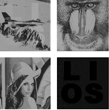
First, we give the original images that will be used in the paper (Figure 3): Lena, airplane, baboon and the secret image. The size of the four images is 256×256; they will be scaled to their proper size when necessary.

Figure 3: The original share images (airplane, baboon and lena) and the secret image.

We provide two well-known objective numerical measurements for the visual quality, the peak signal-to-noise ratio (PSNR) and the universal quality index (UQI) [30]. In this paper, the PSNR is adopted to assess the distortion of each share image with its original halftoned share image (i.e. without the darkening process). In such a way, the PSNR values in Table 9 and 10 can reflect the effects of a combination of the following possible processes in EVCS’s: Darkening, embedding and modification. The PSNR is defined as follows,

𝑃 𝑆𝑁𝑅= 10 log_𝑀𝑆𝐸2552 (2)

where MSE is the mean squared error (MSE). The UQI is adopted to assess the distortion of each share image with its original grey-scale share image (after being scaled to the size of shares). Hence, the UQI value can reflect the effect of the halftoning process besides that of the darkening, embedding and modification processes in EVCS’s. The formal definition of UQI can be found in [30]. In this paper, the block size of UQI is set to be 8 for all the experiments.

The original halftoned share images of the proposed schemes, here, are generated by applying Algorithm 1 on the original share images in Figure 3 directly, and the dithering matrix that is used during the halftoning process of each original share image, after being halftoned, is the same as that is used in the proposed scheme respectively. The original halftoned share images of the Zhou et al. and Wang et al.’s schemes in Figure 5 are generated by the blue noise halftoning technique and error diffusion halftoning technique on the original share images in Figure 3 directly.

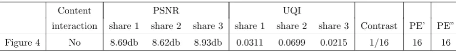
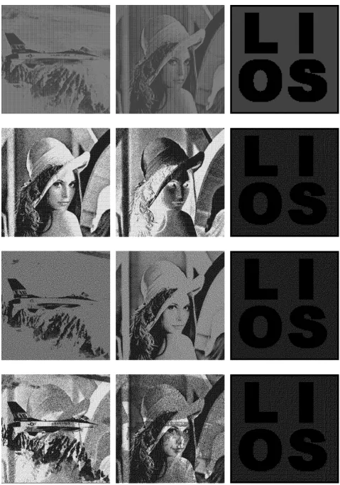
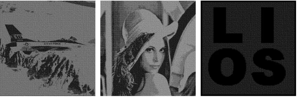
We give two experimental results for the Construction 6, where the black ratio is reduced. The three images of Figure 6 are the experimental results of an embedded (2,2)-EVCS, where the stacking of the two shares on the left will be the recovered image on the right. The share pixel expansion and secret image pixel expansion are 9 and 9 respectively. The contrast of the recovered secret image is 1/9. The PSNR and UQI values can be found in Table 10. Figure 4 show the experimental results of an embedded (3,3)-EVCS1_{, where the stacking of the shares airplane,}

baboon and lena is the recovered secret text “LOIS”. The share pixel expansion and secret image pixel expansion are 16 and 16 respectively. The contrast of the recovered secret image is 1/16. The PSNR and UQI values can be found in Table 9.

Figure 4: The shares and the recovered secret image of an embedded (3,3)-EVCS after reducing the black ratios, the image size is 1024×1024.

Then we give the experimental results (Figure 5 and 6) to compare the visual quality of the shares between the proposed scheme and several well-known schemes proposed in [15–17, 23, 25], where, for each scheme, the stacking of the two shares on the left will be the recovered image on the right. The corresponding pixel expansions, contrast, PSNR and UQI values of each scheme can be found in Table 10.