A normalization circuit of attention in primate lateral prefrontal cortex

(1)

Western University Western University

Scholarship@Western

Electronic Thesis and Dissertation Repository

6-11-2018 1:00 PM

A normalization circuit of attention in primate lateral prefrontal

cortex

Lyndon Duong

The University of Western Ontario

Supervisor

Martinez-Trujillo, Julio C.

The University of Western Ontario

Graduate Program in Physiology and Pharmacology

A thesis submitted in partial fulfillment of the requirements for the degree in Master of Science © Lyndon Duong 2018

Follow this and additional works at: https://ir.lib.uwo.ca/etd Part of the Neurosciences Commons

Recommended Citation Recommended Citation

Duong, Lyndon, "A normalization circuit of attention in primate lateral prefrontal cortex" (2018). Electronic Thesis and Dissertation Repository. 5407.

https://ir.lib.uwo.ca/etd/5407

This Dissertation/Thesis is brought to you for free and open access by Scholarship@Western. It has been accepted for inclusion in Electronic Thesis and Dissertation Repository by an authorized administrator of

(2)

i

Abstract

The way in which visual neurons encode information pertaining to a cluttered scene with

multiple stimuli, and subsequently filter behaviorally relevant information using attention

remains poorly understood. Neurons of area 8a in the macaque lateral prefrontal cortex

have been shown to encode visual and attentional signals. We trained two macaque

monkeys in a visuospatial attention task and performed neurophysiological recordings to

test how neurons in this area encode multiply presented stimuli and attentionally filter

target stimuli from distractors. We found area 8a neuronal responses to several

concurrently presented stimuli to resemble the average of individual responses to those

stimuli when presented alone; this nonlinear response is characteristic of divisive

normalization, a canonical brain computation seen to operate in various neural systems.

Interestingly, the strength of normalization was dependent on visuospatial tuning, with

neurons tuned for the ipsilateral visual hemifield displaying stronger normalized responses

than those tuned for the contralateral hemifield. Furthermore, when presented with

multiple stimuli and attending toward a target stimulus lying in the receptive field,

contralateral-tuned neural activity increased and resembled that of when the target was

presented alone (i.e. Winner-take-all response), whereas ipsilateral-tuned neurons were

less modulated by attention and remained best-described by an average response. Taken

together, our findings suggest a normalization circuit underlying attention in the primate

lateral prefrontal cortex.

Keywords

Attention, Macaque, Prefrontal Cortex, Neural Computation, Neurophysiology,

(3)

ii

Co-Authorship Statement

As at the time of submission, this thesis comprises work submitted as a journal article

currently under review. The contributors to this submitted paper are Lyndon Duong,

Florian Pieper, and Julio Martinez-Trujillo. LD analyzed the data and wrote the paper; FP

(4)

iii

Acknowledgments

The completion project would not have been possible without support from my friends and

family. I owe my deepest gratitude to my mom, dad, Kim, and Tino for their love and

encouragement throughout my degree. It is due to their hard work and sacrifices in their

lives that I have the privilege to pursue my passion in mine.

In the JMT lab, I’d like to thank: Roberto Gulli for his never-ending support, whether it be

scientifically, emotionally, or at the gym; Matthew Leavitt for the continuous supply of

laughter; Benjamin Corrigan for being my conduit for meme-sharing; Guillaume Doucet

for absolutely nothing; Nour Malek for her infinite love and optimism; Theda Backen for

all the fun times hanging together and for her warmth and friendship; Borna Mahmoudian

for listening to my incessant JM fangirling, and words of encouragement to get me through

tougher times. By far, the greatest part of working in this lab has been the lifelong

friendships I’ve made.

Finally, I’d like to thank my supervisor Dr. Julio Martinez-Trujillo for his unconditional

support and guidance despite my wayward. His relentless passion and enthusiasm for his

work continue to inspire me, and have ultimately influenced me to continue my studies in

(5)

iv

List of Figures

Figure 1 Experiment and recordings. ... 12

Figure 2 Response normalization in area 8a ... 13

Figure 3 Spatial tuning and normalization ... 16

Figure 4 Receptive field properties and normalization ... 18

Figure 5 Neuronal responses with directed visuospatial attention. ... 20

Figure 6 Single neuron dynamics of attention ... 22

Figure 7 Winner-take-all decoding with sustained attention ... 24

(9)

1

Introduction and Literature Review

In their seminal publications dating back to the late 1950s, David Hubel and Torsten Wiesel

inserted microelectrodes into awake anesthetized cat primary visual cortex to record the

activity of single neurons in response to visual stimuli (Hubel & Wiesel, 1959). Through a

series of clever experiments, they characterized visual information processing in single

neurons of the primary visual cortex. For their discoveries and functional characterizations

of visual cortex, they were awarded the 1981 Nobel Prize in Physiology or Medicine and

laid the foundation for the field of visual neurophysiology.

Much progress has occurred in the field of visual neurophysiology in the past 60 years. So

much so that the visual system is the most studied sensory modality in contemporary

systems neuroscience (Maunsell, 2015) -- and not without reason. The importance of vision

in our everyday lives is difficult to overstate. In the primate brain (both human and

non-human), the number of neurons dedicated to vision vastly exceeds the number of those that

are devoted to other sensory modalities (Felleman & Van Essen, 1991). This disproportion

reflects our extreme reliance on vision relative to our other senses.

Today, visual function is explored through a wide array of experimental techniques (e.g.

electrophysiology, magnetic resonance imaging, modeling and simulations, etc.), and

across a range of species (e.g. ferrets, rodents, primates, etc.). Furthermore, experimental

designs have branched out in order to study more complex cognitive functions that are

heavily intertwined with vision such as working memory, decision-making, and attention.

However, albeit the seemingly endless number of possible experiments to study the visual

system, all visual research is aimed to answer the same question: how does the brain

(10)

2

1.1 The Neural Code

Neural computation is the study of how neurons process information. In other words, given

a set of inputs to a neuron, what will its output be? In the domain of visual attention, the

study of neural computation has been used to unveil fundamental theories of how attention

allocates cognitive resources in the brain (Desimone & Duncan, 1995), temporal dynamics

of attentional modulation (Buschman & Kastner, 2015), different forms of attention

(Carrasco, 2011), and mathematical models explaining attentional responses in neurons

(Reynolds & Heeger, 2009; Schwedhelm et al., 2016). Neural computation has also been

integrated into other fields, such as machine learning and artificial intelligence (AI)

(Hassabis, et al., 2017). Fundamental concepts derived from our understanding of neural

computation are the foundation of current state-of-the-art machine learning algorithms,

such as artificial neural networks (ANNs) and deep learning (Bengio et al., 2015). By

implementing neural computations inspired by higher-level cognitive functions, like

attention, models have been built that can perform complex tasks such as identifying

several different objects in a single image (Ba et al., 2014), or searching for and identifying

a small object within a large image (Mnih et al., 2014).

This thesis elaborates on many of these biological neural computations borrowed in

machine learning (LeCun et al., 2015; Yamins & DiCarlo, 2016). For example,

max-pooling operations, whereby a neuron exclusively outputs the maximum value it receives

from several inputs while discarding the rest (i.e. winner-take-all). Another example, which

has been further developed by researchers at Google and is the main neural computation

studied in this thesis, is normalization (Ioffe & Szegedy, 2015).

1.2 Normalization

A neuron’s firing rate response to multiple stimuli can be deceptively complex and

nonlinear. The number of action potentials fired in response to multiple simultaneously

presented stimuli is less than the sum of action potentials elicited when each individual

stimulus is presented alone. In other words, neurons respond sublinearly to multiple stimuli

(J. Maunsell, 2015). This holds true for most visual neurons, save for in some cases such

(11)

3

1966), which are known to linearly sum the responses to two stimuli when presented

together.

One reason for the nonlinear responses by most visual neurons is their intrinsic biological

limitation. Neurons cannot fire a negative amount of action potentials, so there will always

exist a point at which the spiking signal is “clipped” (Carandini, 2005). On the opposite

end of the spectrum, a neuron’s action potential firing rate cannot increase to infinity due

to biophysical and energetic restraints, and must saturate. This lower and upper bound on

firing rate sets a finite bandwidth in which a neuron can operate and encode information.

The neuronal response to multiply presented stimuli can differ dramatically by brain

region. For example, in inferotemporal cortex, the response of a visual neuron to multiple

stimuli can be well explained by an averaging computation (Zoccolan et al., 2005). With

an averaging computation, the response of a visual neuron to multiple stimuli resembles

the average of its responses to singly presented stimuli (J. Maunsell, 2015). In contrast to

this, neurons in the parietal cortex respond with a max-pooling (i.e. winner-take-all)

computation (Oleksiak et al., 2010). In this case, a visual neuron’s response to several

stimuli is best described by its maximum response to any of those constituent stimuli

presented individually.

By the early 1990s, researchers proposed normalization as a neuronal computation to

explain the nonlinear properties of these neuronal responses (Heeger, 1992; 1993).

Normalization is not governed by one single, clean-cut equation, but rather is an umbrella

term referring to a class of operations relating response values to some baseline (J.

Maunsell, 2015). Broadly defined, normalization is when a neuron outputs the sum of its

excitatory inputs scaled by the sum of its excitatory and inhibitory activity inputs.

Generally speaking,

(12)

4

constant to avoid divide-by-zero error. Normalization allows neurons to maximize their

sensitivity and efficiently use their entire dynamic range of firing rate. Also, the effective

firing rate rescaling accomplished via normalization may enhance discrimination among stimuli, allowing the encoded information to be read-out (e.g. by a downstream neuron,

linear classifier, etc.) with higher accuracy (DiCarlo & Cox, 2007; Ringach, 2010). Finally,

normalization can allow a neuronal population to flexibly operate between an averaging

regime when inputs to a neuron are approximately equal, and a max-pooling (i.e.

winner-take-all) regime where a neuron selects the maximum of its inputs (Busse et al., 2009;

Riesenhuber & Poggio, 1999). Interestingly, attention, the main cognitive process studied

in this thesis, and normalization may interact to shift a neuron from an averaging to a

winner-take-all computation, thereby allowing it to select the subset of inputs that are most

behaviorally relevant, while suppressing the rest.

1.3 Visual Attention

The phenomenon of attention has been studied by psychologists and neuroscientists for

over 120 years (James, 1890). As the field of attention research has grown, so too has the

number of different attention research subfields. While several brain areas are implicated

in attentional modulation, a complete understanding of its underlying functional

neurophysiology remains unknown.

1.3.1 Types of Attention

Attention can generally be divided into either top-down or bottom-up (Kastner &

Ungerleider, 2000; Treue, 2003). The former can be described as volitional, or

goal-directed allocation of attention. For example, attentively waiting for a traffic light to turn

green. Bottom-up attention, on the other hand, is more reflexive, or stimulus-driven. An

example of this would be one’s reaction to a fire alarm going off unexpectedly. Although

these two forms of attention are distinct, the line between the networks governing them is

blurred (Buschman & Miller, 2007), yet their interaction is necessary for optimal survival

(13)

5

Attention can also be categorized as overt or covert attention. Whereas covert attention is

when one directs attention towards an object or region of space in our periphery (e.g.

avoiding obstacles while texting and walking simultaneously), overt attention is when one

reorients themselves or their gaze to the attended stimulus (Carrasco, 2011; Kastner &

Ungerleider, 2000). Naturally, we tend to reorient our gaze to salient stimuli and thus use

overt attention more frequently in everyday life. In contrast, most experimental paradigms

examining the effects of attention restrict the subject to solely employ covert attention. By

doing so, visual input through the retina is controlled, and/or electrophysiological

recordings are stabilized.

Visual attention can further be classified based on the type of information that is filtered.

Attending to a specific location of the visual field is defined as spatial attention. An

example of this would be when you are focusing on the road while driving. The area that

spatial attention covers can vary from small and focused, to large and dispersed (Laberge

& Brown, 1986; J. J. H. Reynolds & Heeger, 2009). As one increases the area of spatial

attention, information processing becomes less efficient (Castiello & Umilta, 1990; Eriksen

& St. James, 1986). Feature-based attention filters specific features in the visual field such

as texture, color, or motion (Carrasco, 2011), e.g. avoiding the black licorice flavored jelly

beans in a bowl. Finally, object-based attention selects a combination of features to

selectively filter a specific object in our environment, such as searching for a fork in a

drawer of cutlery (Carrasco, 2011; Olson, 2001).

While attention is classified based on the type of information being processed, all types

share one defining characteristic: enhanced perception towards the attended stimulus. In a

classical visual attention study, Michael Posner (1980) showed that reaction times of a

subject’s response to a stimulus are quickened by allocating attention towards it. In this

study, a subject was seated in front of a computer screen, with their gaze fixated in its

center. The subject was given a cue indicating whether an upcoming stimulus would appear

on the left or right side of the screen. When this stimulus appeared on screen, the subject

was to saccade towards it as quickly as possible. This initial cue had a variable probability

(14)

6

opposite location. Posner found that saccade reaction times towards the correct stimulus

were systematically faster with increasing cue validity.

1.3.2 Neural Correlates of Attention

The preferential processing of an attended stimulus occurs at the expense of other stimuli,

whether the relevant stimulus be feature-, object-, or spatial-based. Indeed, complementary

to the effect of enhanced perception of attended stimuli, researchers have also found that

perception of objects and events happening outside the attentional focus are suppressed

(Rock et al., 1992; Simons & Chabris, 1999). This filtering implies that irrelevant sensory

information entering through the retina is somehow disregarded or ignored somewhere

along the visual processing streams (Mack & Rock, 1998). The underlying neuronal

mechanisms of this filtering have been well-studied in the visual system through the use of

in vivo single neuron recordings (Green, 1958; Hubel, 1957).

One of the earliest findings in the study of attention using in vivo electrophysiology was

the modulation of action potential firing rates of visual area V4 and inferotemporal neurons

when attention was directed towards a preferred target located within the receptive field of

a neuron (Moran & Desimone, 1985). Complementing these results, the researchers also

found that a neuron’s firing rate was reduced when attention was allocated to a

non-preferred stimulus within its receptive field. These results were observed across several

areas in visual cortex, including inferotemporal area (Chelazzi et al., 1993; Zhang et al.,

2011), middle temporal and medial superior temporal areas (Treue & Maunsell, 1996), and

V2 (Reynolds et al., 1999), demonstrating that action potential firing rate modulation may

be a neural mechanism by which the competition for neural processing could be biased in

favour of relevant stimuli (Reynolds & Chelazzi, 2004).

In addition to changes in absolute firing rate modulation, neurophysiological studies have

found that attention may enhance the signal of the attended stimulus by regulating other

variables of neural activity. These effects include changes in visual receptive fields

(Connor et al., 1997); increases in phase synchrony between specific bands of local field

potential and locally spiking neurons (Fries et al., 2001), or local field potential activity in

(15)

7

(Mitchell et al., 2007; Sundberg et al., 2009); and decreases in correlated spiking variability

between neurons (i.e. noise correlations; Cohen & Maunsell, 2009).

1.4 The Lateral Prefrontal Cortex

Although it is overwhelmingly clear that visual attention implicates several cortical areas

of the visual system, the origin of the attentional signal is still up for debate. Since the

effects of attention on neural responses become more pronounced as one moves towards

higher-order areas of the visual processing system (J. H. R. Maunsell & Cook, 2002;

O’Connor et al., 2002; Treue, 2001, 2003), several higher-order brain structures have been

suggested as source centers for attention, including: the prefrontal cortex (Miller & Cohen,

2001), the parietal cortex (Bisley & Goldberg, 2010), and even midbrain (Krauzlis et al.,

2014) or thalamic structures (Shipp, 2004). However, recent findings suggest a principal

role for the prefrontal cortex—the “hierarchical superior area” (Felleman & Van Essen,

1991). For example, it has been shown that neural activity in the prefrontal cortex is related

to top-down signals of attention (Buschman & Miller, 2007), and that neurons in the ventral

pre-arcuate region of the prefrontal cortex are causally implicated in feature-based attention

(Bichot et al., 2015).

The lateral prefrontal cortex (LPFC) comprises areas 8A, 8B, 9, 9/46, 10, 46, and 47

(originally defined by Brodmann, 1909; updated by Petrides & Pandya, 1999). This thesis

focuses on neurons recorded in area 8A.

Prefrontal area 8a is anatomically situated anterior to the frontal eye fields (FEF) and

between the principal and arcuate sulci (Petrides & Pandya, 1999). Ensembles of neurons

and/or local field potentials in this area are known to encode visuospatial attention

information (Tremblay et al., 2015; 2016). Single neurons in this area show selectivity for

both visual hemifields, thereby allowing area 8a to encode a spatially complete map of the

visual field (Bullock et al., 2017; Funahashi & Bruce, 1989; Leavitt, Mendoza-Halliday, et

al., 2017; Lennert & Martinez-Trujillo, 2013). This contrasts with the lateral intraparietal

(16)

8

the contralateral visual hemifield (Bushnell et al., 1981; Patel et al., 2010; Thompson,

2005).

Recent work characterizing the visual responses of single neurons in this area have reported

a subset of cells that exhibited firing rate suppression when a single stimulus was presented

in the location opposite its zone of activation (Bullock et al., 2017); interestingly, these

suppressed cells were, for the most part, tuned to the ipsilateral hemifield. In a similar vein,

Lennert & Martinez-Trujillo (2011, 2013) found a difference in temporal dynamics

between ipsilateral- and contralateral-tuned neurons. In this thesis, we extend these

findings by characterizing differences in neuronal responses to multiple stimuli with and

without attentional modulation between these two populations with opposite spatial

preference. The involvement of area 8a in visuospatial attention is clear; however, the exact

sensory and attentional neuronal computations have yet to be determined for cells in this

area.

1.5 Sensory Normalization and Attention

In the biased competition model of attention, proposed by Desimone and Duncan (1995), objects in the visual field each compete for cognitive processing. The limited neuronal

resources available for information processing can be biased towards specific objects by

allocating attention toward them.

Reynolds and Heeger (2009) proposed an extension to the normalization model to account

for the firing rate modulation effects of visual attention. In their model, attention is

implemented via a multiplicative factor, resulting in an enhanced stimulus drive

(excitation) before normalization. This enhanced stimulus drive can substantially bias the

response of a neuron toward the attended stimulus, and can result in a winner-take-all

operation. Thus, a normalization model can capture the effect of biased competition. Put

simply,

(17)

9

where Ratt-pref is a neuron’s response with attention directed toward its preferred stimulus,

with attentional gain, α, acting as a multiplicative gain on its excitatory drive, E. However, this multiplicative increase in excitation (numerator) is limited in its effect due to its

simultaneous contribution to the normalization factor (denominator), which includes the

sum of excitatory as well as (indirect) inhibitory inputs, I. This framework can also capture the effects on neural firing rates when attending toward a non-preferred stimulus. Consider

the neural response of one neuron while attending toward its non-preferred stimulus:

𝑅_{𝑎𝑡𝑡−𝑛𝑜𝑛𝑝𝑟𝑒𝑓} = 𝐸 𝐸 + 𝛼𝐼 + 𝜀

It should be noted that one neuron’s non-preferred stimulus will inevitably be another neuron’s preferred stimulus. Thus, when attending toward a non-preferred stimulus of a

given neuron, as in the equation above, an attentional gain is instead applied to the excited

activity of a separate neural population tuned to this attended stimulus. This ultimately

influences I in our example neuron’s normalization factor (denominator), and thus reduces its overall activity.

The amount of attentional modulation in a neuron can be measured by comparing its

attended responses between its preferred and non-preferred stimulus when both are

presented simultaneously. In the normalization model of attention, attention alters only the

inputs to the normalization rather than altering the normalization mechanism itself. In other

words, attention plays a role in gating the inputs, and normalization lies in a subsequent

stage of processing after attentional modulation (J. Maunsell, 2015).

Recent work by Maunsell and colleagues further explored the relationship between

normalization and attention in area MT of the Macaque (Lee & Maunsell, 2009; Ni &

Maunsell, 2017; Ni et al., 2012). As similarly described in other areas, the authors found

that MT neural responses to a preferred stimulus were reduced when presented with a

non-preferred stimulus even if the non-non-preferred stimulus elicited an excitatory response.

However, for certain cells, a non-preferred stimulus had no effect on firing rate when paired

with the preferred stimulus. The non-preferred stimulus was unable to engage a

(18)

10

normalization responses can be explained if the normalization mechanism itself were

tuned. Tuned normalization would only be engaged by stimuli similar to a neuron’s

preferred stimulus. Consequently, attentional modulation was negligible when shifted

between preferred and non-preferred stimuli in these cells. Normalization can thereby

effectively amplify attention-related modulations, and can account for the differences in

magnitude of attentional modulation between neurons (J. Maunsell, 2015).

This thesis examines the neural activity recorded from prefrontal area 8a of two healthy

male macaque monkeys performing a visuospatial attention task on a computer. Using

chronically implanted microelectrode arrays, we examined single-neuron responses to one

visual stimulus or several visual stimuli to characterize the effects of normalization in this

area. Further, we analyzed each neuron’s subsequent responses when the monkeys were

required to covertly attend to specific stimuli while ignoring others. Finally, we pooled

neural responses to assess the information coding of attention at the level of the neuronal

(19)

11

Results

We investigated how single cells of opposite spatial preference in area 8a process multiple

stimuli and attentionally filter extraneous information in favour of behaviorally relevant

information. Neuronal responses to multiple stimuli with and without directed covert

attention were compared against responses to those stimuli when presented in isolation.

We found that the population response to many stimuli without attention was sublinear and

well-described by an averaging computation; however, the degree to which each individual

neuron’s response was suppressed, relative to a linear response, varied with spatial tuning.

Specifically, we found ipsilateral-tuned neurons to be more suppressed than

contralateral-tuned neurons. We then compared time-averaged and time-varying responses to the same

array of stimuli when attention was directed toward and away from a neuron’s receptive

field (RF) center. Attending toward the RF center modulated contralateral-tuned neuronal

firing rates toward a winner-take-all regime, whereas ipsilateral-tuned neuronal firing rates

were less modulated and remained better explained by an averaging computation.

2.1 Experimental Task and Recordings

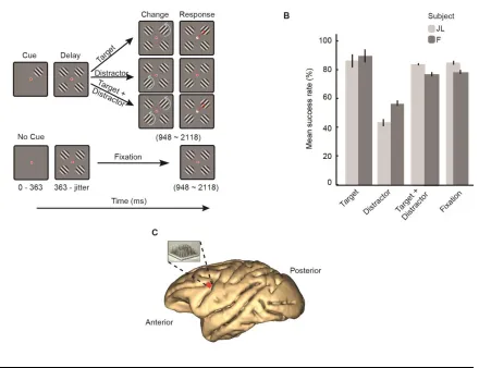
We trained two male macaque monkeys to direct gaze to (fixate) a dot at the center of a

screen and covertly attend to a grating stimulus (the target) located in one of four possible

screen quadrants while ignoring distracters located in the other quadrants. The location of

the target was indicated by a cue appearing at the beginning of every trial. When the target

changed orientation, the animal made a saccade towards it (attention trials; Figure 1A top).

These attention trials were randomly interleaved with trials of a fixation condition (fixation

trials), in which no cue stimulus was presented, the four stimuli appeared simultaneously

on the screen and the animal was required to detect a change in the fixation point contrast

(Figure 1A bottom). Both subjects learned and successfully performed the task well above

chance level of 25% (Figure 1B). We implanted one multielectrode array (Utah array,

Blackrock Microsystems, UT) in the left dorsolateral prefrontal cortex of each monkey

(20)

12

the animals performed the tasks. We isolated 458 single units across 23 recording sessions

(248 units across 11 recording sessions in monkey F, 210 units across 12 recording sessions

in monkey JL). Using firing rates computed in each trial during the Cue epoch and

sustained attention (Delay) epoch, we found that 236 (51%) of these units were tuned for

both the cue location (sensory tuning) and the allocation of spatial attention (attentional

(21)

13

primarily focused on the 236/458 single units across all recording sessions that were both

cue and delay selective.

2.2 Normalization in Area 8a

In our task, the cue was presented alone in one of four quadrants on a computer screen at

the beginning of attention trials; this allowed us to examine the responses of the neurons to

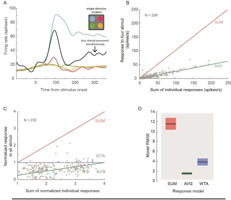
Figure 2 Normalization in area 8a. A) Example single unit (77_jl_149_u14) firing rate responses to four singly presented stimuli (colored lines) and the same four stimuli presented simultaneously (black line). B) Multiple vs. single stimuli responses. Each grey point is the sum of a unit’s spiking responses to four individually presented stimuli vs. its firing rate when those four stimuli were presented simultaneously. The red and green lines are predictions of linear additive (SUM) and

averaging (AVG) responses, respectively. C) Winner-take-all (WTA) computation. Points are

(22)

14

single stimuli presented in different quadrants of the visual field. The responses during

fixation trials allowed us to quantify the responses to all the stimuli when presented

together. Figure 2A shows an example neuron with a typical response to singly and

multiply presented stimuli. In general, found that the visual responses of area 8a single

neurons toward multiple stimuli did not equal the sum responses to those stimuli presented

alone, as predicted by a linear summation model (Figure 2B, SUM, red line). Indeed, the

vast majority of our tuned units’ (232/236; 98%) responses to multiple stimuli were

sublinear and resembled an averaging response (AVG, green line). To further explore this,

we transformed the data in Figure 2B by scaling each unit’s response by the mean response

to its preferred stimulus (Figure 2C). This enabled the comparison of responses to a

winner-take-all response model prediction (WTA, blue line) wherein a unit’s response to

multiple stimuli equals its response to that of its preferred stimulus alone, i.e., the stimulus

that evoked the largest response. We computed the root mean square error (RMSE) of the

data to the prediction of the three different models (see Materials and Methods). Of these

three response configurations, the AVG computation described the responses best, yielding

the lowest RMSE for this population of isolated units (bootstrap, p < 0.05, Bonferroni

corrected). This demonstrates that neurons in area 8A undergo response normalization

when multiple stimuli are presented in the visual field.

2.3 Spatial Tuning and Normalization

From our previous studies, we found tuning-dependent differences in sensory and attention

responses of units in this area. Specifically, units that were tuned to the ipsilateral or

contralateral visual hemifield, relative to the recording site, exhibited dissociable dynamics

during sensory and attention tasks (Lennert & Martinez-Trujillo, 2013). Furthermore, we

have reported spatial tuning-dependent varying degrees of firing suppression when

presented with single stimuli (Bullock et al. 2017). We sought to extend these findings by

characterizing the tuning-dependent responses to multiple stimuli with and without

attentional modulation.

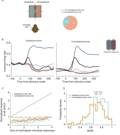
We divided our sample into neurons that produce the maximal response when the single

(23)

15

neurons that produce the maximal response when the stimulus was presented

contralaterally to the recording hemisphere (contralateral units) (Figure 3A, B). Figure 3C

shows the same plot as Figure 2B, but with each unit labeled according to visuospatial

tuning. By comparing RMSE between models, we found that both subpopulations of tuned

units were best described by an averaging response (bootstrap t-test p<0.05, Bonferroni

corrected). We quantified the strength of normalization in each unit with a Multiple

Stimulus Response Index (MSRI),

where rall is a unit’s average response to the four stimuli presented simultaneously, and ri

is its average response to a single cue stimulus presented in quadrant i on the screen.If a unit’s response to many stimuli is greater than that of the sum of its responses to those

stimuli presented individually, MSRI is less than 0. If a unit response to all stimuli (rall)

equals the sum of the responses to each stimulus alone (∑ri) then MRSI is 0. If rall is greater

than ∑ri , MSRI is less than 0. If rall is lower than ∑ri MSRI is between zero and 1. For our

task with four stimuli presented simultaneously, MSRI = 0.75 is an averaging response

(AVG). Although the distributions of MSRI of the two tuned populations overlap, the

average MSRI was greater for ipsilateral-tuned units (median = 0.78, 95% CI [0.75, 0.81])

than for contralateral-tuned units (median = 0.70, 95% CI [0.67, 0.73]; Mann-Whitney-U

test, z = 4.32, p = 7.97x10-6), indicating a greater response normalization in

ipsilateral-tuned units when presented with multiple stimuli (Figure 3D).

2.4 Neuron Receptive Field Properties

These differences in normalization responses could possibly be explained by differing

receptive field (RF) properties between units, such as RF size. Here we consider the RF as

the region of the visual field that is modulated by the appearance of the single cue and

includes both excitatory (RFe) and inhibitory (RFi) regions. To investigate this issue, we

estimated the size of each unit’s receptive field by examining whether individually

(24)

pre-16

Figure 3 Tuned neural visual responses. A) Individual units categorized by visual spatial tuning relative to recording site. B) Average estimates of continuous firing rates (spike density functions) for ipsilateral-tuned (left panel) and contralateral-tuned (right panel) populations. Colored lines are average population responses to single stimuli presented in one of four possible quadrants; stimuli were shown inside a unit’s preferred quadrant (i.e. the stimulus which elicited a maximal response; solid blue), in a quadrant adjacent to the unit’s preferred quadrant in the same visual hemifield (dotted blue), opposite visual hemifield (solid red), or located in the quadrant located diagonal to the preferred quadrant (dotted red). Black lines are average population responses to these four stimuli when presented simultaneously. C) Same as 2B), but with units classified by their spatial tuning. Bootstrapped moving averages for each tuned population are displayed for visualization purposes

(10,000 samples; window size 0.2; step size 0.05). D) Histograms of Multiple Stimulus Response

(25)

17

stimulus baseline response (Figure 4A; paired t-test, p<0.05, Bonferroni corrected). On

average, ipsilateral-tuned units had RFs spanning more quadrants of the visual field

(median = 3 quadrants) than contralateral-tuned units (median = 2 quadrants;

Mann-Whitney-U test, z = 3.02, p = 0.003). However, the overall size of a unit’s receptive field

was weakly correlated with its MSRI (Spearman rho = 0.18, p= 0.006; Figure 4B), and

thus it is unlikely to fully account for the differences in normalization strength between the

two subpopulations.

The differences in normalization between the two oppositely tuned populations may be

related to the composition of the RF. Specifically, the suppressed response to many stimuli

may depend on whether specific regions of the RF are excitatory or inhibitory, as assessed

by the response to the single cue relative to baseline. Indeed, in our recorded population

we obtain a heterogeneous sample of RF compositions (Figure 4C, purely inhibited, mixed

and purely excited).

We found that whereas the size of a unit’s RFe was negatively correlated with the MSRI

(Spearman rho = -0.34, p = 1.3x10-7), the size of the RFi was positively correlated with the

MSRI (Spearman rho = 0.50, p = 5.2x10-16). Thus, when the RF contains larger inhibitory

regions (quadrants, in our case), the cell is more likely to show a stronger normalization

response. Conversely, when the RF contains more excitatory regions, it is less likely to

show a stronger normalization response. In agreement with this result, on average the

MSRI for purely inhibited neurons was the highest and for purely excited neurons the

(26)

18

Figure 4 Receptive Field Properties. A) Distributions of receptive field sizes for ipsilateral and contralateral neurons. A quadrant of the visual field was classified as being part of a unit’s receptive field if a singly presented stimulus in that quadrant elicited a response (excitatory or inhibitory)

different from pre-stimulus baseline (paired t-test; p < 0.05 Bonferroni corrected). B)

Corresponding MSRI of units with a given receptive field size. Medians (black vertical lines) were computed using 10,000 bootstrap samples and grey bars indicate the 2.5 and 97.5 percentile confidence intervals of the distribution of medians. Confidence intervals for top row: [0.65, 0.72]; second row: [0.66, 0.76]; third row: [0.73, 0.81]; and fourth row: [0.71, 0.76]. C) Receptive field configurations. Singly presented stimuli may either excite or suppress neuronal activity relative to baseline. Thus, the receptive field of a given neuron can be 1) a purely inhibitory, 2) a purely excitatory, or 3) a mixture of both. D) Corresponding MSRI of units with RF compositions shown in C). MSRI was greater in units with a greater proportion of inhibitory receptive quadrants. Each dot is one single unit. Dots are horizontally jittered with reduced opacity for clarity. Vertical length of diamonds are 2.5 and 97.5 percentile confidence intervals of the bootstrapped distributions (10,000 samples) of medians. Confidence intervals for purely inhibited cells: [0.79, 0.83]; cells with a mixture of excited and inhibited activity: [0.73, 0.79]; and purely excited cells: [0.64, 0.68].

2.5 Effects of Attention on Area 8a Neuronal Responses

During attention trials, presented stimuli were identical to those presented during fixation

trials. However, after the cue presentation, when the four stimuli appear on the screen, the

(27)

19

three distractors located in the other quadrants (Figure 1A, top). We characterized neuronal

responses when attention was allocated toward the stimulus that evoked a stronger response

when presented alone (preferred stimulus, “Attend In”), toward the other non-preferred

stimuli (“Attend Out”), and the Fixation trial, when none of the four stimuli were cued

(“Fixation”). Single unit average spike rasters were convolved with a Gaussian kernel (15

ms standard deviation), and z-scored yielding spike density functions (SDFs) during the

Delay epoch for the ipsilateral population (Figure 5A; left panel), and contralateral

population (right panel).

For a given neuron, firing rates were on average higher during “Attend In” trials (Figure

5A, blue line) than “Attend Out” trials (Figure 5A, red line). This effect was highly

significant for both the ipsilateral-tuned population (t-test, t(68) = 5.5, p = 6.2 x 10-7) and

contralateral-tuned population (t-test, t(162) = 7.15 , p = 2.8 x 10-11) and may be interpreted

as a shift in the description of the population response, from an average (AVG) to a

winner-take-all (WTA) regime.

To test this hypothesis, we examined this effect separately for the populations of ipsilateral

and contralateral units. Interestingly, we found that “Attend In” responses of contralateral

units were better described by a WTA model than when compared with the population of

ipsilateral units (Figure 5B). In this figure, a linear regression slope of 1 signifies a WTA

response. The regression slope for contralateral units (median slope = 0.89; 95% CI [0.81,

0.96]). was greater than that of the ipsilateral units (median slope = 0.62; 95% CI [0.59

0.65]; bootstrap t-test, p < 10-4). The abscissa of Figure 5C is identical to that of Figure

3C; however, the ordinate now represents a unit’s “Attend In” response. We computed the

RMSE corresponding to each model prediction for contralateral and ipsilateral and for

“Attend In” and “Attend Out” conditions (Figure 5C). “Attend In” and “Attend Out”

responses of ipsilateral units remained best-described by AVG model (Figure 5D;

bootstrap t-test, p = 3x10-4). For contralateral units, “Attend Out” responses were also

(28)

20

(29)

21

described by an AVG model (bootstrap t-test, p=3x10-4_{). However, “Attend In” responses}

were best described by a WTA response (dashed grey box; bootstrap t-test, p = 0.01)

indicating that when the animals attended to the preferred location or stimulus, contralateral

units shifted from an AVG to a WTA regime. This suggests that contralateral units showed

a stronger modulation of responses with attention relative to ipsilateral units.

2.6 Dynamics of Sustained Attention

The previous analyses used firing rates averaged over a time period of the task, when the

animals directed attention to the target and ignored the distractors. We next examined the

temporal dynamics of the attentional modulation in contralateral and ipsilateral-tuned

units. We scaled each unit’s SDF shown in Figure 5A by the mean response to its preferred

stimulus (i.e. maximal response) to yield a time-evolving Winner-take-all index (WTA

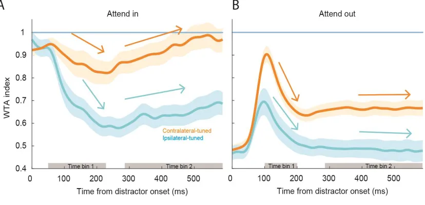
index, Figure 6).

During the “Attend In” condition (left panel) following distractor onset, both population

responses were attenuated. We computed the decay slopes of each population response

(Figure 6A; linear regression slopes computed during the left grey region, time bin 1) and

found the ipsilateral neurons slope (cyan arrow; time bin 1) to be more negative than the

contralateral neurons’ slope (orange arrow; time bin 1) (mean ± std. dev.: -2.0 ± 0.3 s-1 vs.

-0.8 ± 0.3 s-1; bootstrap t-test p = 8x10-4). This shows that during “Attend In” trials,

ipsilateral neurons were more strongly suppressed by the appearance of the distractors than

contralateral neurons. Following this initial response decrease, there was an upward trend

(computed during the right grey region, time bin 2) towards a WTA response (dashed line),

with the average slopes corresponding to both populations being positive, but not

statistically different from one another (orange and cyan arrows bin 2) (ipsilateral-tuned

slope: 0.3 ± 0.1 s-1; contralateral slope: 0.4 ± 0.1 s-1; bootstrap t-test p = 0.18). This suggests

that the rate of change of spiking activity towards the WTA regime during the delay period

when the animals sustained attention on the target is similar in both populations. However,

the degree of suppression by distractor onset preceding the sustained attention period is

(30)

22

During “Attend Out” trials, neural activity initially ramped up towards the WTA line for

both populations, however this increase was greater in magnitude for the

contralateral-tuned units (Figure 6B; bootstrap t-test, p<1x10-4). After this initial increase, the activity

promptly decreased in both populations. The rate of decay (linear regression slope during

time bin 1) for both contralateral- and ipsilateral-tuned populations were similar

(ipsilateral-tuned slope: -1.4 ± 0.5 s-1; contralateral-tuned slope: -2.0 ± 0.4; bootstrap t-test

p = 0.12). After the fast decay in response, firing rates stabilized (Figure 6B; time bin 2),

linear regression slopes were not different from zero for either the ipsilateral-tuned

(bootstrap t-test, p = 0.42) or contralateral-tuned population (bootstrap t-test, p=0.86). The

level at which ipsilateral units stabilized was significantly lower than the one at which

contralateral units stabilized (both relative to the WTA line). This is likely a direct

consequence of the initial response increase being stronger in contralateral-tuned relative

to ipsilateral-tuned units.

Figure 6 Single neuron characterization of attention dynamic responses. Bootstrapped

average population Winner-take-all index over time for A) “Attend In” and B) “Attend Out”

(31)

23

2.7 Winner-take-all Decoding with Sustained Attention

Whether these tuning-dependent differences in normalization and attentional modulation

affect the ensemble code of spatial attention is unknown. Indeed, the translation from single

neuron coding to population coding is non-trivial (Leavitt, et al., 2017; Moreno-Bote et al.,

2014). However, it is possible to use classification methods to assess information content

pertaining to spatial attention in these ensembles. Specifically, we used decoders to

measure the similarity between neural activity when attention was directed toward an

object surrounded by distractors (Delay epoch) to the activity when that object was

presented in isolation (Cue epoch). This allowed us to directly evaluate whether sustained

attention gave rise to a WTA computation at the level of the population.

To test this, we used a linear classifier to decode the locus of spatial attention during the

Delay epoch. We constructed 1000 pseudopopulations of 232 neurons by randomly

sampling 100 trials from each of the 4 task conditions (4 possible cue locations) for each

neuron. We trained a model on each pseudopopulation’s average firing rates integrated

over a 300ms window during the Cue epoch (same time window as in previous analyses;

see Materials and Methods), and tested the trained model on average firing rates during a

300ms window of the Delay epoch. The classifier treats each vector of single neuron firing

rates as a feature with each entry (trial) being an independent observation. Using 232 single

neurons, the classifier achieved decoding accuracy of 87±2% (Figure 7A, pink line, firing

rate computed during grey time bin). This shows that the population response with attention

toward an object in the presence of distractors is highly similar to that of when the object

was presented alone, suggesting an attentionally modulated WTA computation.

We further quantified the dynamics of this state similarity using the same classifier trained

on Cue epoch 300 ms time bin firing rates; however, we evaluated the time-evolving state

similarity by using sliding windows of mean firing rates during the Delay epoch as a test

set (Figure 7A, blue curve). We used 25 ms backwards-looking boxcar windows stepped

by 25 ms to compute firing rates from the spiking raster data. We repeated this analysis

with varying window sizes, and found similar results (see Materials and Methods).

(32)

24

level (25%). However, the decoding accuracy recovered and increased towards

approximately 60% shortly thereafter, and continued to steadily increase with a linear

regression slope of 0.02 ± 0.01% ms-1_{(mean ± standard deviation) with sustained attention}

(Figure 7B, blue arrow, regression computed using grey shaded region). This slope was

significantly different from zero and positive (bootstrap t-test, 1000 samples, p<0.001).

therefore, with sustained attention the pattern of neural ensemble coding of the attended

stimulus evolves to resemble that of when the stimulus is presented alone.

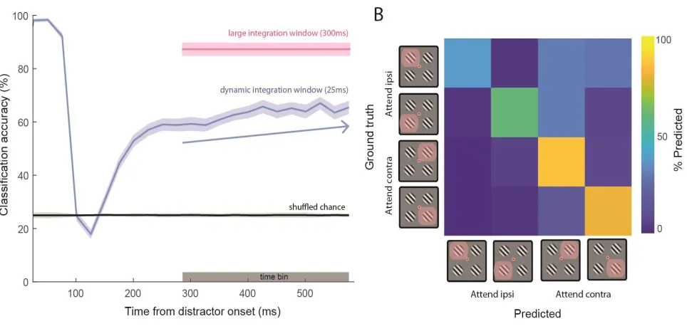
Figure 7 Winner-take-all decoding with sustained attention. A) Linear classifier using a pseudopopulation of 232 single unit firing rates trained on the latter 300 ms of the Cue epoch, then tested on: i) firing rates computed in a large 300 ms time window (pink shaded error bar, using grey time bin to compute firing rate), and ii) dynamic, trailing moving windows during the Delay epoch (window = boxcar with width 25 ms; step size = 25 ms). We repeated this procedure 1000 times, sampling 100 trials from each of the four trial conditions with replacement for each neuron. Solid lines are mean classification accuracy, and shaded error is one standard deviation of entire bootstrapped sample. Classification accuracy slowly increased after recovery from transient activity (linear regression computed on dynamic classification accuracy during time bin denoted by grey

shaded region) with a slope of 0.02 ± 0.01 ms-1_(mean_±_{standard deviation; blue arrow). B) Example}

(33)

25

We show a representative confusion matrix derived from test-set predictions made by a

decoder at the final time point of the blue curve in Figure 7B. Interestingly, these models

on average made a greater number of classification errors for trials in which attention was

allocated toward the ipsilateral field than when attention was directed toward the

contralateral field (50%+/-1 vs 80%+-/1; bootstrap t-test p<0.05). This demonstrated that

when attending toward a stimulus in the presence of distractors, the population read-out of

information relevant to the contralateral hemifield is more effective than that of the

ipsilateral hemifield. This is likely a resulting effect of the varying differences in magnitude

of attentional modulation between the ipsilateral- and contralateral-tuned populations.

2.8 Decoding the Locus of Spatial Attention During the

Delay Epoch

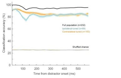
Lastly, we examined the available information relevant to the allocation of spatial attention

during the Delay epoch itself (Figure 8). We trained three linear classifiers to decode the

locus of covet spatial attention. These decoders were trained on: ipsilateral-tuned firing

rates, or contralateral-tuned firing rates, or both subpopulation firing rates together. We

trained these decoders on short-duration windows and tested on firing rates during the same

window, and repeated this over the duration of the Delay epoch (stepped by 25 ms).

We systematically tested firing rates computed in different time window sizes ranging from

5 ms to 35 ms, in 5 ms increments (see Materials and Methods). First, we noted that using

time windows as low as 25 ms to compute firing rate, the decoders reached classification

accuracies of greater than 95% on average (Figure 8, black curve). Secondly, classification

accuracies using each subpopulation’s firing rates (Figure 8, orange and blue curves) both

decreased following distractor onset, with the magnitude of decrease being greater in the

ipsilateral-tuned population than contralateral-tuned population (bootstrap t-test p<0.001).

This was likely due to the greater suppressed response in ipsilateral-tuned cells.

Interestingly, both subpopulations converged toward the same level of classification

accuracy (bootstrap t-test p>0.05), despite there being a larger subpopulation of

contralateral-tuned neurons (163 neurons) than ipsilateral-tuned neurons (69 neurons). This

(34)

26

in size for each neuron) between the two tuned populations; however, we repeated these

analyses while controlling for receptive field size and found similar results (not shown).

(35)

27

Discussion

This study systematically characterized neural responses to multiple objects with in lateral

prefrontal area 8A of the macaque monkey. We also investigated information coding

during the allocation of attention within this area at two levels, single cell responses and

neuronal ensembles. By comparing neuronal responses to single and multiple stimuli

without directed attention, we found that a neuron’s response to many stimuli was

well-described by an averaging computation as well-described in many areas of cortex. Furthermore,

the magnitude of normalization of a given unit’s response to multiple stimuli (relative to a

SUM response) was related to its visuospatial tuning; ipsilateral-tuned neuron responses to

multiple stimuli were more normalized than contralateral-tuned neuron responses.

Attention differentially modulates the firing rates of these two subpopulations of

contralateral and ipsilateral neurons shifting the population code from average to

winner-take-all; however, this effect is stronger in the population of contralateral neurons. Finally,

ensembles of neurons with opposite spatial preferences for the contralateral and ipsilateral

visual hemifields interact to facilitate better decoding of the location spatial attention,

demonstrated by a linear classifier reaching performance near 100% in correctly performed

trials.

3.1 Normalization in Area 8a

In normalization models of attention, attending toward an object shapes the information

inputs to a neuron by applying a gain to the attended input (Boynton, 2009; Ghose, 2009;

Lee & Maunsell, 2009; J. J. H. Reynolds & Heeger, 2009); importantly, this stage occurs

as a separate step prior to normalization (A. Ni et al., 2012). Therefore, it was critical for

us to understand and characterize the default normalization response in neurons without

The vast majority (232/236; 98%) of recorded visually and attentionally modulated neurons

exhibited a sublinear response best characterized by an averaging computation when

(36)

28

response to many stimuli resembles the average of responses to those stimuli when

presented alone; this finding has been reported in multiple areas across visual cortex (e.g.

Britten & Heuer, 1999; Recanzone et al., 1997; Zoccolan et al., 2005; and Maunsell, 2015

for a review). One consequence of this normalization would be to maximize each neuron’s

sensitivity, allowing them to efficiently use their available dynamic range in firing rates to

encode objects in the visual field before the allocation of attention (Carandini & Heeger,

2012). As the PFC is thought to play a key role in top-down attention, it is imperative that

neurons in this area maintain an appropriate bandwidth in which they may encode stimulus

information prior to allocating attention. As multiple stimuli appear in the visual field,

normalization rescales the activity of these neurons, preventing their firing rates from

saturating. As a result, their activity can still be modulated by attention, allowing them to

effectively encode the locus of attention for a downstream read-out. This averaging

response in area 8a contrasts the default winner-take-all rule reported in area 7a of the

posterior parietal cortex, perhaps reflecting the role of the PFC in top-down attention, and

parietal cortex in bottom-up attention (Oleksiak et al., 2010).

3.2 Receptive Field Properties and Response

Normalization

Neurons in this area are known to possess large receptive fields tuned for either visual

hemifield (Bullock et al., 2017; Funahashi & Bruce, 1989; Mikami et al., 1982). Indeed,

here we report neurons with receptive fields spanning up to four quadrants of the visual

field (Figure 4). Interestingly, the absolute size of a neuron’s receptive field was weakly

correlated to MSRI, and thus could not fully explain a neuron’s suppressed response to

many stimuli. If the normalization mechanism itself were tuned in this area, as was

proposed in other parts of cortex (Carandini et al., 1997; Ni et al., 2012; Rust et al., 2006),

then this could help explain the varying degrees of recorded normalized responses among

neurons. In this framework, individual stimuli can influence normalization to varying

degrees, even allowing stimuli that elicit no response when presented alone to contribute

to normalization. Stimuli lying outside of a given neuron’s receptive field, which excite a

separate population of neurons, could thereby suppress its overall activity when presented

(37)

29

We found that the responses to multiple stimuli of area 8a neurons were related to the

excitatory or inhibitory nature of their receptive fields. Specifically, neurons with stronger

normalization responses tended to possess receptive fields with more inhibitory regions

than excitatory regions. This is likely due to non-preferred stimuli increasing the inhibitory

drive to a neuron, which results in a larger normalization factor (Carandini & Heeger,

2012).

3.3 Spatial Tuning Preference and Normalization

A recent study mapping visual receptive fields in area 8a showed a difference in receptive

field composition between contralateral- and ipsilateral-tuned neurons (Bullock et al.,

2017). The authors used a series of singly presented stimuli to assess receptive field

structure and function, and found ipsilateral-tuned neurons to possess more inhibitory

receptive fields than those with opposite spatial tuning. Our findings extend this study by

also characterizing area 8a neuronal responses to multiple stimuli. In corroboration with

their work, we found that ipsilateral-tuned neurons exhibited more strongly suppressed

activity than contralateral-tuned neurons when presented with many stimuli (Figure 3, 4).

We believe this can be explained by the disproportion of neurons selective for the

contralateral hemifield. Indeed, our findings of ~70% contralateral representation (and

~30% ipsilateral) in area 8a is in agreement with previous studies in this area (Bullock et

al., 2017; Lennert & Martinez-Trujillo, 2013). As stimuli populate both hemifields,

competition-driven mutual suppression to either population of oppositely tuned cells is

uneven due to this skewed representation of the contralateral field. Thus, in response to

multiple stimuli spanning the entire visual field, the inhibitory drive to the ipsilateral

population was larger, due to there being more contralateral neurons than ipsilateral

neurons. This would result in the strength a stronger normalization response, resulting in

more suppressed responses compared to those of the contralateral-tuned population.

3.4 Attentional Modulation Varies Between Populations of

Oppositely Tuned Neurons

Attending toward the center of the RF increased the activity of both tuned subpopulations

(38)

30

on the recorded contralateral-tuned neurons, with responses resembling a winner-take-all

computation while ipsilateral-tuned neurons remained better characterized by an averaging

computation (Figure 5). In normalization models of attention, attention acts as a

multiplicative gain on the drive of the attended stimulus prior to normalization (Ghose,

2009; Lee & Maunsell, 2009; J. J. H. Reynolds & Heeger, 2009). As with neural responses

during fixation trials (without allocated attention), the mutually inhibitory interactions

were unequal between these subpopulations due to the greater proportion of

contralateral-tuned neurons. Therefore, despite the increase in excitatory drive to ipsilateral-contralateral-tuned

neurons when attention was allocated toward the ipsilateral hemifield, the presence of

distractors in the contralateral hemifield contributes to a larger normalization factor for the

ipsilateral population. Conversely for contralateral-tuned neurons, the inhibitory

interactions stemming from distractors in the ipsilateral field contributed less to

normalization. This may have resulted in the greater increase in firing rates in the

contralateral neurons (toward winner-take-all).

3.5 Dynamics of Attentional Modulation and Normalization

The rapid dynamics of normalization and attentional modulation remain poorly understood

(J. Maunsell, 2015). In this study, we showed that during Attend In trials, the amount and

rate by which spiking activity was suppressed after distractor onset differs between

contralateral- and ipsilateral-tuned neurons (Figure 6). Specifically, ipsilateral-tuned cell

activity was suppressed farther and at a faster rate than that of the contralateral-tuned

population. Following sensory perturbation caused by the distractor onset, both populations

tended toward a Winner-take-all state at similar rates as attention was sustained. These

dynamics may be explained under the normalization framework; normalization models

capture the bottom-up distractor response, as in the responses during fixation trials, with

top-down attention subsequently adjusting the weighting to the attended stimuli (Reynolds

& Heeger 2009). The asymmetry in mutually inhibitory inputs may result in the greater

magnitude and faster dynamics of suppression in the ipsilateral-tuned population. The

ensuing attentional modulation increased the firing rate of either population at the same

(39)

31

ipsilateral-tuned population, their responses could not reach a winner-take-all state with

Although the temporal dynamics of the “Attend Out” responses did not differ between the

two subpopulations, the absolute magnitude of suppression did (Figure 6, right panel).

Whereas ipsilateral-tuned neural activity returned to a state equal to baseline activity (when

there was no excitation whatsoever), the suppression of activity in the contralateral-tuned

populations plateaued at a higher level. These suppressive responses during “Attend Out”

conditions are consistent with the general understanding that attention filters behaviorally

irrelevant information in favor of relevant information. If the encoding of irrelevant

information should be discarded, then the population response while attending to a stimulus

surrounded by distractors should resemble the population response to that stimulus when

presented in isolation, i.e. Winner-take-all (Moran & Desimone, 1985; Zhang et al., 2011).

This can only be achieved by suppressing the activity of neurons which are excited by the

unattended distractors.

3.6 Information Content of Spatial Attention at the Level of

the Population

The translation from single neuron responses to ensemble coding and information read-out

is nontrivial (Moreno-Bote et al., 2014). Using linear classification methods allowed us to

quantify the evolution of population state similarity to when the attended stimulus was

presented alone (i.e. Winner-take-all). A study using similar methods to these found

attentional modulation to drive the responses of inferotemporal neurons toward a

Winner-take-all state (Zhang et al. 2011).

We found that a classifier trained on neuronal firing rates during the Cue epoch could be

used to reliably decode, with high accuracy, the location of covert spatial attention during

the Delay epoch (Figure 7). This showed that the population response to a stimulus

presented in isolation explained much of the variance of the population response when

attending to that stimulus in the presence of distractors. This finding was consistent with

attentional modulation yielding a Winner-take-all response, and corroborates the theory of

A normalization circuit of attention in primate lateral prefrontal cortex

Scholarship@Western

Scholarship@Western

A normalization circuit of attention in primate lateral prefrontal

A normalization circuit of attention in primate lateral prefrontal

cortex

cortex

Abstract

Keywords

Co-Authorship Statement

Acknowledgments

Table of Contents

List of Figures

Introduction and Literature Review

1.1

The Neural Code

1.2

Normalization

1.3

Visual Attention

1.3.1

Types of Attention

1.3.2

Neural Correlates of Attention

1.4

The Lateral Prefrontal Cortex

1.5

Sensory Normalization and Attention

Results

2.1

Experimental Task and Recordings

2.2

Normalization in Area 8a

2.3

Spatial Tuning and Normalization

2.4

Neuron Receptive Field Properties

2.5

Effects of Attention on Area 8a Neuronal Responses

2.6

Dynamics of Sustained Attention

2.7

Winner-take-all Decoding with Sustained Attention

2.8

Decoding the Locus of Spatial Attention During the

Delay Epoch

Discussion

3.1

Normalization in Area 8a

3.2

Receptive Field Properties and Response

Normalization

3.3

Spatial Tuning Preference and Normalization

3.4

Attentional Modulation Varies Between Populations of

Oppositely Tuned Neurons

3.5

Dynamics of Attentional Modulation and Normalization

3.6

Information Content of Spatial Attention at the Level of

the Population