Magnetic Induction Tomography with High Performance
GPU Implementation
Lu Ma1, Robert Banasiak2, and Manuchehr Soleimani1, *
Abstract—Magnetic induction tomography (MIT) is a non-invasive medical imaging technique with promising applications such as brain imaging and cryosurgery monitoring. Despite its potential, the realisation of medical MIT application is challenging. The computational complexity of both the forward and inverse problems, and specific MIT hardware design are the major limitations for the development of MIT research in medical imaging. The MIT forward modeling and linear system equations for large scale matrices are computationally expensive. This paper presents the implementation of GPU (graphics processing unit) for both forward and inverse problems in MIT research. For a given MIT mesh geometry composed of 167,488 tetrahedral elements, the GPU accelerated Biot-Savart Law for solving the free space magnetic field and magnetic vector potential is proved to be over 200 times faster compared to the time consumption of a CPU (central processing unit). The linear system equation arising from the forward and inverse problem, can also be accelerated using GPU. Both simulations and experimental results are presented based on a new GPU implementation. Laboratory experimental results are shown for a phantom study representing potential cryosurgery monitoring using an MIT system.
1. INTRODUCTION
Magnetic Induction Tomography (MIT) is the most recent and least developed electrical tomography technique. It does not require electrical contact with the body and instead uses the interaction of an oscillating magnetic field with a conductive medium. The field is excited by inductive coils with an alternating current, which are arranged around the region of interest (ROI). Eddy currents arise when a conductive object is present within the sensing zone, which causes a perturbation to the magnetic field. The passive electromagnetic properties of the object under testing can be reconstructed from the degree of perturbation of this field. It is important to note that MIT is sensitive to conductivity, permeability and permittivity; however, sensitivity to conductivity is usually the primary focus for research [1].
In MIT, the relationship between the field perturbation and the primary magnetic field can be expressed by ΔBB ∝ω(ωε0εr−jσ) [2], where it can be seen that perturbation of the secondary magnetic
field is proportional to the square of the frequency. If the object is highly conductive, such as metal, the field perturbation ΔB is dominated by a negative imaginary part. Therefore, the measurements can be taken from the amplitude of the imaginary part, as the real component is negligible. For biomedical applications, the conductivity of biological tissues is many orders of magnitude lower than that of metals and they have no appreciable permeability above that of free space. Therefore, both the real and imaginary parts need to be taken into consideration. This paper presents the reconstruction of a non-conductive inclusion in a low conductive background, which has an electrical conductivity of 1.58 S/m. This might be of interest in medical applications, for example, cryosurgery, where undesired tissues need to be frozen as part of the treatment [3–7]. Human tissues have conductivity values less than 2 S/m; in this context, frozen cells/tissues can be considered non-conductive [8, 9], and as such this
Received 19 October 2015, Accepted 19 December 2015, Scheduled 2 January 2016
* Corresponding author: Manuchehr Soleimani ([email protected]).
1 Engineering Tomography Laboratory (ETL), Department of Electronic and Electrical Engineering, University of Bath, BA2 7AY,
conductivity contrast can be used for imaging. The aim of this study is to provide insight as to how MIT can be of general use for medical applications as a non-destructive tomographic technique. In this paper, both simulations and experimental results are presented.
In the area of tomographic research, there are usually two problems which need to be solved, the forward problem and the inverse problem. Both problems can be computationally expensive and time consuming, resulting in a growing demand for advanced computing techniques to accelerate the solving process. This could be of particular use in brain/lung function imaging as the finite element model could incorporate up to millions of elements [10–13]. It has also been shown that the calculation of Jacobian matrix is the most expensive computing process in the forward solver [14], especially for 3D tomography approaches. As a result, the implementation of graphics processing units (GPU) has gradually gained popularity [15]. The implementation of GPU techniques has been investigated in the area of both hard-field [16] and soft-hard-field tomography [14] to achieve computational gain, including electrical impedance tomography (EIT) [17] and electrical capacitance tomography (ECT) [18]. Compared to the use of GPU in previous MIT research [19, 20], where the parallelisation of the finite difference (FD) algorithm was achieved, in this work, the time reduction using GPU is realised differently. An edge finite element method (FEM) is used to solve the forward model, which involves generating the meshes, solving the magnetic vector potential and fields in every single tetrahedral element, as well as solving the system linear equation which is a large scale sparse matrices calculation. In the algorithm section, a high performance computation is achieved using GPU implementation, which improved the computational efficiency in solving both MIT forward and inverse problems.
2. METHODS
2.1. Measurement System
The MIT system used for this study consists of (i) a coil array of 16 equally spaced air-core sensors, (ii) a National Instrument (NI) based data acquisition system and (iii) a host computer. The sensing zone has a diameter of approximate 25 cm, each coil has 6 turns, a side length of 1 cm, and a radius of 2 cm. Figure 1 shows the medical MIT system used in this study. Among 16 coils, 8 coils are engaged for transmitting signals, and the remaining 8 coils are dedicated for receiving signals; the total number of independent measurements is therefore 64. A grounded aluminium cylinder is used to prevent external electric field perturbation. As the signal perturbation caused by the secondary magnetic field is usually low for a MIT system, the measurement system requires accurate measurement devices to improve the sensitivity. ANI2953 is employed to realise the multi-channel switching process. The measured data are collected, combined and displayed through aNI5781 device. In order to improve the system efficiency, aNI7951 FlexRIO board is utilized to accelerate the data acquisition process. An excitation frequency of 13 MHz is chosen for this system. The sampling rate of this system is 100 megasamples/s. The image reconstruction module extracts 64 independent measurements to perform the reconstruction algorithm, displays and updates the images through the LabView and Matlab programs. A detailed description of the system design and evaluation of driving signal level, phase noise and phase drift have been reported in [21].
2.2. Forward and Inverse Problem
In this study, a reduced magnetic vector potential is used to avoid modelling the structure of the coils using edge FEM [22, 23]. In the (A,A) formulation we have:
∇ × 1
μ∇ ×A+jσωA=Js (1)
where the current density, Js, can be prescribed by the magnetic vector potential according to the Biot-Savart Law.
The magnetic potential constitutes two parts A = As+Ar, where As represents the impressed magnetic vector potential as a result of current source Js, and Ar represents the reduced magnetic
vector potential in the eddy current region Ωe. In the non-conductive region Ωn:
∇ ×Hs=Js (2)
where Hs is the magnetic field generated by an excitation coil, which can be directly computed from
any point P in a free space fromJs:
Hs=
Ωn
Js(Q)×rQP
4π|rQP|3 dΩQ (3)
whererQP is the vector pointing from the source pointQto the field pointP. The impressed magnetic vector potentialAs can be written by:
∇ ×As=μ0Hs (4)
From Equation (3) and Equation (4),As is readily shown as:
As=
Ωn
μ0Js(Q)
4π|rQP|2dΩQ (5)
In the entire region Ωn+ Ωe, using time harmonic and complex notation, the magnetic flux density can be expressed by:
B =μ0Hs+∇ ×Ar (6)
According to Faraday’s Law of induction, ignoring the displacement current, the induced electric field can be written in the following form:
∇ ×E =−jωB (7)
From Equation (6) and Equation (7), the induced electric field in the entire region is:
E =−jωAs−jωAr (8)
Eddy currents arise when a conductor is exposed in a time varying magnetic field; therefore, in the eddy current region Ωe:
Jeddy =σE (9)
In the region of Ωn+ Ωe, the magnetic field can be expressed by:
∇ ×H=Jeddy+Js (10)
It is known that the relationship between B andH is:
B =μH (11)
whereμ is the permeability of the medium.
Combining Equations (2), (6), (8), (10) and (11), we have:
∇ ×
1
μ∇ ×Ar
+jωσAr =∇ ×Hs−jωσAs− ∇ × 1
μμ0Hs (12)
boundary conditions. In edge FEM on a tetrahedral mesh, a vector field is represented using a basis vector functionNij associated with the edge between nodes iandj:
Nij =Li∇Lj−Lj∇Li (13)
where Li is a nodal shape function. Applying the edge element basis function to Galerkin’s
approximation [24, 25], one can obtain:
Ωe
∇ ×N· 1
μ∇ ×Ar
dv+
Ωe
jωσN ·Ardv =
Ωc
(∇ ×N·Hs)dv−
Ωc
(N ·jωσAs)dv
−
Ωc
1
μμ0∇ ×N·Hs
dv (14)
whereN is any linear combination of edge basis functions, Ωe the eddy current region, and Ωc the coil region. It can be seen from Equation (14) that the right hand side can be solved by Equations (3) and (5), the only unknown variable is the reduced vector potential Ar. By applying edge FEM, the
second order partial differential equations can be computed by a combination of system linear equations, which can then be processed through Matlab. Ar can be obtained using the BiConjugate Gradients
Stabilized Method to solve the system linear equation [26]:
SAr=b (15)
where S = Sr+jSi, which is a complex matrix; b is the current density, which is also complex. By solving the reduced magnetic vector potential Ar, one is able to evaluate the induced voltages in the measuring coils. The induced voltages can be calculated by using a volume integration form:
Vmn=−jω
Ωc
A·J0dv (16)
whereA=As+Ar, and J0 is a unit current density passing through the coil.
The sensitivity matrix is essential in MIT as it realises the linearisation between the conductivity and the induced voltages. The elements of the Jacobian matrix can be expressed by [27, 28]:
∂Vmn
∂σk =−ω
2
ΩkAm·Andv
I0 (17)
whereVmnis the measured voltage,σkthe conductivity of pixelk, and Ωkthe volume of the perturbation (pixel k). Am and An are respectively solutions of the forward solver when the excitation coil m is excited byI0 and the sensing coil nexcited with unit current. It is worth mentioning that if the object under testing has a significant relative permittivity εr, the imaginary term jωε0εr must be added to the complex conductivity. In this case, the complex conductivity can be written as ξ=σ+jωε0εr.
The inverse problem usually makes use of the forward model as part of the solving process. Let the forward model be expressed in a linear approximation.
V =Jσ (18)
where V is a column vector consisting of M voltage measurements and σ also a column vector representingK pixels. J is anM×Kmatrix of the sensitivity map, calculated from Equation (17). The inverse problem is solved to compute the distribution of the conductivity through measured voltages. In most cases, this is an underdetermined problem as the number of measured voltages is far less than the number of pixels, resulting in the solution being ill-posed. In order to ensure the uniqueness and the stability of the solution, the least square solution (LSS) is applied.
minV −Jσ2 = min(V −Jσ)T(V −Jσ) (19) ∂
∂σ
the Tikhonov regularisation method is used to solve the inverse problem, where the reconstruction relies on the fact that for small changes, the measurements can be approximated in a linear fashion with a regularisation parameterα and regularisation matrixR [29].
σ=JTJ+αR −1JTV (22)
2.3. GPU High Performance Computing
2.3.1. Parallelisation Scheme
The computation of both forward and inverse problems for MIT is time consuming, and as such, there is a pressing need to accelerate it. One approach is to adapt and convert MIT data processing into parallel computing architectures. There are two possible ways to achieve this goal: the classic parallel solution, i.e., running on multiple CPU (central processing unit) cores, and the GPU (graphics processing units) solution. The former uses multi-node PC (personal computer) systems to perform one global task by splitting it into subtasks. This method is well established, requiring a specialised software, a low-latency network infrastructure to exchange data between nodes and an increased hardware complexity. The latter uses the parallel architecture of GPUs, through a novel technique called GP GPU (General-Purpose computing on Graphics Processing Units) (http://gpgpu.org).
A growing interest in GPU computation began in general with the difficulty in clocking CPUs above a certain level due to the limitations of silicon-based transistor technology. Although sequential programs are easier to understand, the growing demand for improvements in modern computing led to an increased interest in multi-core technology and parallel architectures [30, 31]. Nevertheless, even with parallel architectures, there is still a limit as to how fast programs can run. Speed increases are now based primarily on improving the architecture of the CPU rather than higher clock rates [32]. Until recently, parallel programming was reserved for high performance clusters with multiple processors, as the cost was often prohibitively expensive. However, this changed with the introduction of new types of multi-core processor to the mainstream market, including GPUs.
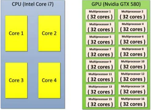
Compared to CPUs which today have a maximum of 2 to 12 cores, GPUs consist of dozens, or even hundreds, of smaller, simpler cores designed for a high level of parallelisation (Figure 2).
CPUs are designed to execute a large set of instructions (which often includes a high level of branching) as fast as possible, while GPUs mostly take care of computations using a more limited instruction set with less branching. For this reason their execution units, or cores, can be much simpler, i.e., smaller. Therefore, a single chip may have dozens or even hundreds of cores on it. Moreover, graphics computations can be easily parallelised in GPU work based on a SIMD (Single Instruction, Multiple Data), or more precisely SIMT (Single Instruction, Multiple Thread) architecture, where the
same instruction can be applied to numerous subsets of data, in effect allowing a large dataset to be processed rapidly. This allows a much higher number of operations per second than can otherwise be achieved on a CPU. Many time consuming computations can now run in close to real-time with a smaller investment in hardware compared to before the advent of GP GPU.
A real breakthrough in the ease-of-use of GP GPU came with the introduction of Nvidia CUDA (Compute Unified Device Architecture) in 2007 (http://docs.nvidia.com). Programmers could then use generic software libraries to exploit the potential of the massively parallel GPU architecture and reduce the running time of many algorithms (http://docs.nvidia.com/cuda/cuda-c-programming-guide/). Nevertheless, GPU computation is not without its limitations. One of the key challenges is that GPUs were originally designed for parallel operations, and as such they will not do well on sequential tasks, or those that involve a lot of branching [30].
In this work, the AccelerEyes Jacket GPU processing toolbox is used to run the calculations in parallel. The Jacket GPU library is a mature solution that uses Nvidia’s CUDA parallel computing libraries and enables the writing and running of code on the GPU in a way similar to how it would be done in the Matlab language. Jacket accomplishes this by automatically wrapping the M-language into a GPU CUDA-compatible form by adapting input data to Jacket’s GPU data structure, Matlab functions can be easily transformed into GPU functions. Jacket also preserves the interpretive nature of the M-language by providing real-time transparent access to the GPU compiler, which increases the efficiency of parallel computing code. A new GPU computing library is also available to be embedded in the standard Matlab engine; however, it is currently at an early stage of development and therefore relatively limited.
2.3.2. GPU Accelerated MIT forward Solver
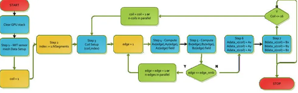
High time consumption due to the expensive computation of the solving process has put constraints on the CPU-based MIT forward solver (Equations (3) and (5)). The magnetic field and magnetic vector potential need to be calculated for every single tetrahedral element, and then integrated over all the elements for a given mesh. This needs to be repeated for every single coil in the MIT forward model (Figure 3). This is a very repetitive process, particularly for a very dense mesh, and as such is both time consuming and computationally expensive. However, all other steps of the MIT forward solution can be efficiently accelerated using a Matlab GPU-based approach.
In this work, a new hybrid type of Biot-Savart equation-solving infrastructure is developed which performs parallel computations using a GPU. The Biot-Savart calculations for Equations (3) and (5) are computed for each individual tetrahedral element in the MIT finite element model without depending on the results of other elements and therefore these can be performed in parallel. Figure 3 depicts this process using a flow chart. Note that there are three main, but completely different in their nature, sequential loops. To properly adapt this kind of iterative algorithm into a GPU parallel scheme, one first
needs to consider the limitations of using the Jacket GPU library. The major drawback is that nested loops are not currently supported. This means that the selection of each loop must be done according to the GPU highly scalable parallel architecture to achieve computational gain. The outermost loop (Steps 1–2) represents a typical CPU-type loop. It computesnnumber of coil segments for an assigned index, wherenis typically much smaller than the total number of elements in a given mesh. In this case, the use of Matlab native CPU vectorisation is an optimal approach because the expense of marshaling the data onto the GPU and retrieving it would not be paid off for a small number of segments (e.g., 2000–5000 segments).
There are two remaining loops that can be adapted into a Jacket parallel scheme (Steps 3–7). The outer loop iterates over the number of coils — here called the “coils” loop — with the number of coils defined asNc (Step 3). This loop includes a second inner loop — called the “edges” loop — defined as a stream of matrix linear algebra computations (additions, subtractions and multiplications) that need to be calculated for a given mesh geometry for a given coil number from the outer loop. The edges loop iterates over a large number of tetrahedral edges that correspond to the density of a given mesh.
There are two choices to accelerate the computation: parallelising either the coils loop or the edges loop. Parallelising the coils loop is an inefficient means of acceleration as each coils loop contains embedded edges loops. In our MIT system, the number of coils, Nc, is 16, but there are hundreds of
thousands of edges. Parallelising the coils loop in this manner can be accomplished just as efficiently as using CPU vector operations. As the GPU computing architecture is internally optimised for a large number of parallel calculations (many cores and many threads), the inner edges loop is selected for GPU parallelisation.
With regards to selecting the edges loop for parallelisation, there are two methods to achieve this goal. One solution is to predefine a Jacket GPU type index variable that iterates over the number of edges, using this predefined index for all variables that need to be iterated in this way. The Jacket GPU vectorisation mechanism is able to use this index to parallelise all algebraic functions and process edge data by hundreds of separate computing threads (and physical cores). Another solution is the use of the in-built Jacket GPU type loop, which looks similar to classic Matlab “for-end” type loop. The difference is that all the GPU loop iterations will run in separate computing threads. To use the GPU loop, all the internal MIT physics functions (Steps 4–7, A, B magnetic field properties computing, edge-based function specified in Figure 3) and edge data must use the same loop (edge number) iterator, which must be defined as a GPU type variable at the beginning of the loop. This approach is the most efficient way of using GPU parallel architecture. One difficulty associated with implementing this innovative computation method is that the GPU code requires that all processing data be transferred into GPU memory at the beginning of the computation, and transferred back to CPU memory at the end of the computation. Repetitious conversion of variables between CPU and GPU type “on-the-fly” (inside loops) is computationally inefficient and can significantly increase the processing time according to the scale of MIT forward and inverse mesh. To avoid this problem, the GPU memory needs to be cleaned and all the data that are going to be parallelised need to be preloaded once into GPU memory before any loop starts.
Table 1 shows the comparison of MIT forward problem processing times for CPU (Inter Core i7 2.8 GHz) and Tesla C2070 GPU. For a mesh geometry composed of 167,488 tetrahedral elements, we achieved a 200x speedup when using a GPU compared to using a CPU alone. It is important to note that these speedups (shown in Table 1) were critically evaluated with careful profiling of CPU and GPU programs and in particular in comparison with multi-CPU systems. This way the computational gain of using GPU can be illustrated, and this speedup increases for denser meshes. In this study, the coil arrangement is fixed, thus the Biot-Savart calculation for the free space field is calculated once; however, for a MIT system where the coil geometry is changing, such as in a rotational MIT system, the coils are rotated according to the rotational scheme, and the forward model needs to be updated accordingly. In this context, the implementation of GPU techniques becomes more advantageous. It is also favorable to use GPU-accelerated Biot-Savart calculations in the forward model when a MIT system has a large number of coils, for instance, 256 coils.
Table 1. Time consumption using CPU and GPU for Biot-Savart calculation for different mesh densities.
Nmb. Mesh density
Biot-Savart Law Intel Core i7, 2.8 GHz
Elapsed time (s)
Biot-Savart Law Tesla C2070 Elapsed time (s)
Gain
1 1797 13.96 0.45 31.02
2 119280 1571.30 11.24 139.80
3 167488 3374.82 16.75 201.48
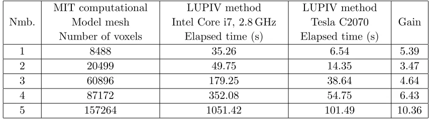
Table 2. Processing times for solving MIT linear system equation using CPU and GPU.
Nmb.
MIT computational Model mesh Number of voxels
LUPIV method Intel Core i7, 2.8 GHz
Elapsed time (s)
LUPIV method Tesla C2070 Elapsed time (s)
Gain
1 8488 35.26 6.54 5.39
2 20499 49.75 14.35 3.47
3 60896 179.25 38.64 4.64
4 87172 352.08 54.75 6.43
5 157264 1051.42 101.49 10.36
for reduced computational times for calculations involving a large number of matrix inversions has motivated the adaption of numerical methods for parallel computing architectures [30], including some for GPU architectures.
Applicable techniques for our method include the BiConjugate Gradients Stabilized Method (BICGS) [33], LU factorisation with partial pivoting (LUPIV) [34] and Gaussian elimination (GE) [35]. The BICGS is optimised for solving large-scale linear system equations in which the system matrices are sparse. This approach is therefore the most efficient for MIT problems whose system matrices are sparse. However, at this stage of research, it is not feasible to use the dense algebra library (Jacket DLA), which leads to the choice of either the LUPIV or GE method to solve Equation (15). We use the built-in Jacket CUDA-optimised LUPIV implementation to maximise performance when running on a GPU to minimize power usage. The comparison of MIT forward problem processing times for CPU and Tesla C2070 GPU are presented in Table 2.
As seen in Table 2 the use of the GPU-adapted LUPIV results in an increase in speed compared to an equivalent CPU implementation. To perform LUPIV computations using the GPU Jacket library, the system matrix needs to be converted from a sparse type to a full type. As the number of system matrix elements is defined by the square of the number of mesh vertices, the full representation of the system matrix can consume gigabytes of memory. For instance, a full representation of the system matrix using mesh model number 5 (Table 2) consumes approximately 4.6 GB of memory. Therefore the Jacket-based LUPIV memory consumption is the major drawback of using this algorithm for a large scale MIT mesh model and it can seriously limit its application. To avoid the problem of memory consumption, the sparse linear algebra and GPU-adapted BICGS algorithm (as stated in Section 2.2) will be applied for further improvement.
2.3.3. GPU Accelerated MIT Inverse Problem
performing addition, subtraction, multiplication and division for matrices. All these algebraic routines are parallelisable, especially multiplication [14, 36]. To improve the efficiency of solving the MIT inverse problem, we use the GPU Jacket library.
To apply GPU to the Tikhonov regularisation, we use a direct method, which is relatively easy to convert to GPU-based structure because the use of the linear matrix equation (Equation (22)). The CPU implementation is able to process this equation in its compact form; however, the GPU conversion requires it be decomposed into fewer simpler and shorter lines. This concept of equation adaptation is crucial for the management of Jacket GPU memory and data processing efficiency. A typical GPU data processing pipeline is optimised using many small linear algebra routines, and as such the efficiency of complex matrix operations is significantly improved. This approach is presented and discussed in Table 3.
Table 3. Fully sequential CPU-based MIT inverse problem vs. hybrid parallel GPU-based MIT inverse problem.
Sequential CPU implementation Parallel GPU implementation
x= (JTJ +αR)−1JTb
AGPU =JT(∗) AGPU =AGPUJ AGPU=AGPU+αR AGPU=inv(AGPU)(∗∗)
BGPU=JT BGPU=BGPUb x=AGPUBGPU(∗ ∗ ∗) The above equation is solved
directly and sequentially from left to right. All linear algebra routines:
multiplication,transposition addition and inversion are processed sequentially by CPU
The input is decomposed into new Aand B temporal variables. Expressions are solved sequentially
from top to bottom. All simplified linear algebra routines are processed in parallel by GPU
Although the sequential CPU approach is simpler and more intuitive, the GPU-based reconstruction is much faster. For example, the GPU-based transposition (*) occurs three orders of magnitude faster than its CPU equivalent [37]. The speed of matrix inversion (**) has been already proved in Table 2. The most efficient line is the last one (***). It includes the matrix multiplication process, which is considered the most efficient parallelised linear algebra transformation [18]. The acceleration of matrix multiplication is huge, up to several hundredfold. The same principles can be applied to other direct reconstruction methods, for example, NOSER (Newton-one-step-error-reconstruction) [38]. There are still no methods for the parallelisation of iterative reconstruction processes, such as the Landweber technique or the Gauss Newton iterations. This is due to the fact that the iterations are not independent of each other. Nevertheless, for an iterative process inside another iterative loop, it is still feasible to accelerate the computation using GPU implementation.
3. RESULTS
The purpose of this section is to demonstrate the feasibility of implementing MIT in a biomedical application, whereby both the solving processes of forward and inverse problems are accelerated using GPU high performance computing technique.
3.1. Simulations
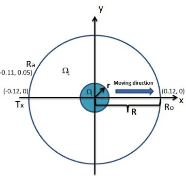
Figure 4. Cross-section of inclusion region Ω1 in the sensing zone Ω2: Tx shows a transmitting coil, Ra and Ro represent the locations of adjacent and opposite measuring coil in relation toTx.
Radius of the inclusion (cm)
0.02 0.03 0.04 0.05 0.06
Normalised induced voltage (V)
× 10
0.4 0.6 0.8 1 1.2 1.4 1.6 1.8
2 adjacent measurement
opposite measurement
Location of the inclusion along x-axis (cm)
0.02 0.04 0.06 0.08 0.10
Normalised induced voltage (V)
0.7 0.8 0.9 1 1.1 1.2 1.3 1.4 1.5 1.6
1.7 adjacent measurement
opposite measurement
(a) (b)
-6 × 10⁻⁶
Figure 5. (a) Normalised induced voltages vs. radius of the inclusion; (b) normalised induced voltages vs. location of the inclusion along x-axis as shown in Figure 4.
volume of the inclusion. In the simulation model, an inclusion of 2 cm radius is located at the centre of the imaging region at the initial state. The conductivity of the background is 1.58 S/m. In all cases, an adjacent and an opposite measurement are simulated in order to show the changes in induced voltages. All the measurements are normalised against the background measurement. The moving direction of the inclusion and the locations of adjacent and opposite coils are shown in Figure 4.
3.2. Experimental Results
In order to investigate the feasibility of using the MIT technique for reconstructing conductivity contrasts in biomedical applications, two sets of experiments are conducted (shown in Figure 6). Increasing the radius of the inclusion in the sensing zone (Figure 6(a)) corresponds to the voltage perturbation in Figure 5(a). The change in displacement of the inclusion from the centre of the sensing region, (Figure 6(b)), corresponds to the voltage perturbation in Figure 5(b). For each case, four different sizes of non-conductive bottle are tested, with diameters of 2, 6.5, 9.5 and 13 cm respectively. As this paper is focused on static 2D reconstructions, the bottles are uniform in the axial direction; therefore, the volume of the inclusion can be approximated by the cross-sectional area of the bottle.
(a) (b)
Figure 6. (a) Increasing the radius of the inclusion in the sensing zone; (b) the change in displacement of the inclusion from the centre of the sensing region.
D = 2 cm D = 6.5 cm D = 9.5 cm D = 13 cm
Figure 7. Reconstructed images of a non-conductive inclusion located in the centre of the measuring region filled with 0.9% saline solution (conductivity of 1.58 S/m). The diameters of the inclusions are 2, 6.5, 9.5 and 13 cm respectively, in columns left to right.
x1= 2 cm x2= 4 cm x3= 6 cm
Figure 8. Reconstructed images of three steps of moving direction of a non-conductive inclusion in the measuring region filled with 0.9% saline solution (conductivity of 1.58 S/m). Reconstructions of inclusion of diameters 13 and 9 cm are shown from the top to the bottom row.
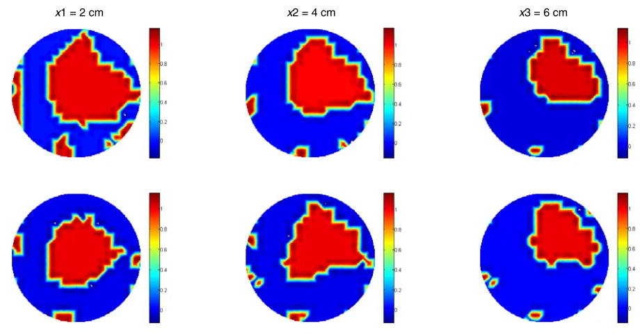
x1= 2 cm x2= 4 cm x3= 6 cm x4= 7 cm
Figure 9. Reconstructed images of three steps of moving direction of a non-conductive inclusion in the measuring region filled with 0.9% saline solution (conductivity of 1.58 S/m). Reconstructions of inclusion of diameters 6.5 and 2 cm are shown from the top to the bottom row.
Figure 8 shows the reconstructed images of non-conductive inclusions moving increasingly off centre in increments of 2 cm. Two different sizes of inclusion are tested — of diameters 13 cm and 9.5 cm — reconstructions of which are shown from the top to the bottom row, of Figure 8 respectively.
Figure 9 shows the reconstructed images of four non-conductive inclusions off centre by 2, 4, 6 and 7 cm, shown in columns left to right, respectively. In addition, two different sizes of inclusion are tested — of diameters 6.5 cm and 2 cm — reconstructions of which are shown from the top to the bottom row, of Figure 9 respectively.
to the low resolution of MIT. Although both simulations and experimental results demonstrate that the reconstruction of high conductive contrast is feasible, further development is essential to fully employ MIT as a useful imaging technique in biomedical applications, where 3D dynamic reconstruction and real-time monitoring are required. In this work, a linear reconstruction algorithm is used to solve the inverse problem. As the experimental data are in 2D, the scale of this problem is relatively small. In addition, the Jacobian matrix is calculated once and used in the inversion as a result of implementing the one step reconstruction algorithm. The reconstructed images shown in Figure 8 and Figure 9 are the proof of principle for potential medical imaging results. In practical cases, if higher resolution of the reconstructed image is required, the Jacobian matrix needs to be updated in an iterative reconstruction process. This way, the advantage of using GPU would be more beneficial in reducing the time consumption. However adapting GPU implementation in an iterative reconstruction algorithm for medical imaging is beyond the scope of this work.
4. CONCLUSION
In this study, a high frequency MIT system is used to study the reconstruction of conductive contrasts, with Tikhonov regularisation used to reconstruct 2D static images. Due to the nature of eddy currents, the MIT forward problem can be a large scale problem, and as such the forward solver is computationally expensive using traditional CPU computation techniques. This problem becomes more severe if the forward model is very dense, i.e., millions of elements, which is common in biomedical applications for brain/lung function imaging. This is one of the key limitations in MIT research. For a 2D problem, the inverse solver can usually be handled by a CPU, however, if the problem is 3D or involves a large number of voxels, this could be inefficient for the solving process.
In this study, both forward and inverse solvers are developed in-house. There are two major challenges in the program pipelines: the calculation of the Biot-Savart law and the calculation of the system linear equation, both of which can be accelerated using GPU implementation. General programming guidance of GPU implementation for Tikhonov regularisation is also presented, which offers computational gain by using matrix decomposition. The overall performance of the GPU implementation can be evaluated from a computational point of view. In order to reconstruct one frame of image, a Biot-Savart law for magnetic field calculation, a linear system equation and an inverse algorithm need to be solved. These take approximately 76%, 23% and<1% of the total computational time, respectively. These estimates are drawn from the last model of Tables 1 and 2, where the sizes of both models are closer to those that would be used in a biomedical application. Considering the gain achieved by using GPU techniques, it is reasonable to believe that high performance computing techniques could reduce the overall processing time by 97%.
Due to the use of the accelerator package Jacket, some information relating to high performance computing is not accessible; however, the parallel implementation of MIT data processing using high level functions, such as transpose, multiplication, subtraction, addition and numerical API for inversion are included.
The aim of this paper is to demonstrate a means by which high performance computing techniques can be used for performance improvement of magnetic induction tomography, especially in the field of medical imaging. Although the model used in this study is a relatively simple 2D model, both the simulations and experimental results show that this GPU-based implementation can achieve uncompromising performance. One could also argue that the performance of GPU-based implementation in MIT would be further enhanced in more sophisticated 3D biomedical models. Future study will expand the scope of this paper to include the implementation of GPU for: i) inverse solution to Krylov subspace based methods, such as conjugate gradient and its preconditioning; ii) various regularisation methods such as total variation for a large scale 3D MIT; iii) detailed profiling, parallelisation scheme, and architecture for such implementations.
REFERENCES
2. Griffiths, H., W. R. Stewart, and W. Gough, “Magnetic induction tomography: A measuring system for biological tissues,” Annals of the New York Academy of Sciences, Vol. 873, 335–345, 1999. 3. Otten, D. M. and B. Rubinsky, “Cryosurgical monitoring using bioimpedance measurements
— A feasibility study for electrical impedance tomography,” IEEE Transactions on Biomedical Engineering, Vol. 47, No. 10, 1376–1381, 2000.
4. Soleimani, M., O. Dorn, and W. R. B. Lionheart, “A narrow-band level set method applied to eit in brain for cryosurgery monitoring,”IEEE Transactions on Biomedical Engineering, Vol. 53, No. 11, 2257–2264, 2006.
5. Zlochiver, S., M. M. Radai, M. Rosenfeld, and S. Abboud, “Induced current impedance technique for monitoring brain cryosurgery in a two-dimensional model of the head,” Annals of Biomedical Engineering, Vol. 30, 1172–1180, 2002.
6. Zlochiver, S., M. Rosenfeld, and S. Abboud, “Contactless bio-impedance monitoring technique for brain cryosurgery in a 3D head model,”Annals of Biomedical Engineering, Vol. 33, No. 5, 616–625, 2005.
7. Ma, L., H.-Y. Wei, and M. Soleimani, “Cryosurgical monitoring using electromagnetic measurements: A feasibility study for magnetic induction tomography,” 13th International Conference in Electrical Impedance Tomography, 2012-05-23–2012-05-25, Tianjin University, Tianjin, 2012.
8. Gabriel, C., A. Peyman, and E. H. Grant, “Electrical conductivity of tissues at frequencies below 1 MHz,” Physics in Medicine and Biology, Vol. 54, No. 16, 4863–4878, 2009.
9. Gencer, N. G. and M. N. Tek, “Imaging tissue conductivity via contactless measurements: A feasibility study,” Elektrik, Vol. 6, No. 3, 183–200, 1998.
10. Bagshaw, A. P., A. D. Liston, R. H. Bayford, A. Tizzard, A. P. Gibson, A. T. Tidswell, M. K. Sparkes, H. Dehghani, C. D. Binnie, and D. S. Holder, “Electrical impedance tomography of human brain function using reconstruction algorithms based on the finite element method,”Neuro Image, Vol. 20, No. 2, 752–764, 2003.
11. Hwu, W.-M. W.,GPU Computing Gems, Emerald Edition, Morgan Kaufmann, 2011.
12. Steuwer, M. and S. Gorlatch, “High-level programming for medical imaging on multi-GPU systems using the skelcl library,” 2013 International Conference on Computational Science, Vol. 18, 749– 758, 2013.
13. Shi, L., W. Liu, H. Zhang, Y. Xie, and D. Wang, “A survey of gpu-based medical image computing techniques,” Quantitative Imaging in Medicine and Surgery, Vol. 2, No. 3, 188–206, 2012.
14. Borsic, A., E. A. Attardo, and R. J. Halter, “Multi-GPU jacobian accelerated computing for soft field tomography,” Physiological Measurements, Vol. 33, 1703–1715, 2012.
15. Eklund, A., P. Dufort, D. Forsberg, and S. M. LaConte, “Medical image processing on the GPU: Past, present and future,”Medical Image Analysis, Vol. 17, No. 8, 1073–1094, 2013.
16. Jia, X., B. Dong, Y. F. Lou, and S. B. Jiang, “GPU-based iterative cone-beam CT reconstruction using tight frame regularization,” Physics in Medicine and Biology, Vol. 56, No. 13, 3787, 2011. 17. Tavares, R. S., T. C. Martins, and M. S. G. Tsuzuki, “Electrical impedance tomography
reconstruction through simulated annealing using a new outside-in heuristic and GPU parallelization,” Journal of Physics Conference Series, Vol. 407(Conference 1), 012015, 2012. 18. Kapusta, P., M. Majchrowicz, D. Sankowski, and R. Banasiak, “Application of GPU parallel
computing for acceleration of finite element method based 3D reconstruction algorithms in electrical capacitance tomography,”Image Processing and Communications, Vol. 17, No. 4, 339–346, 2013. 19. Maimaitijiang, Y., M. A. Roula, S. Watson, R. Patz, R. J. Williams, and H. Griffiths,
“Parallelization methods for implementation of a magnetic induction tomography forward model in symmetric multiprocessor systems,”Parallel Computing, Vol. 34, No. 9, 497–507, 2008.
21. Wei, H.-Y. and M. Soleimani, “Hardware and software design for a national instrument-based magnetic induction tomography system for prospective biomedical applications,” Physiological Measurement, Vol. 33, No. 5, 863–879, 2012.
22. B´ır´o, O., “Edge element formulations of eddy current problems,” Computer Methods in Applied Mechanics and Engineering, Vol. 169, 391–405, 1999.
23. B´ır´o, O. and K. Preis, “An edge finite element eddy current formulation using a reduced magnetic and a current vector potential,”IEEE Transactions on Magnetics, Vol. 36, No. 5, 3128–3130, 2000. 24. Golias, N. A., C. S. Antonopoulos, T. D. Tsiboukis, and E. E. Kriezis, “3D eddy current computation with edge elements in terms of the electric intensity,” The International Journal for Computation and Mathematics in Electrical and Electronic Engineering, Vol. 17, No. 5/6, 667–673, 1998.
25. Barber, D. C. and B. H. Brown, “Applied potential tomography,” Journal of Physics E: Scientific Instruments, Vol. 17, No. 9, 723–734, 1984.
26. Soleimani, M. and W. R. B. Lionheart, “Absolute conductivity reconstruction in magnetic induction tomography using a nonlinear method,” IEEE Transactions on Medical Imaging, Vol. 25, No. 12, 1521–1530, 2006.
27. Dyck, D. N., D. A. Lowther, and E. M. Freeman, “A method of computing the sensitivity of the electromagnetic quantities to changes in the material and sources,” IEEE Transactions on Magnetics, Vol. 30, 3415–3418, 1994.
28. Soleimani, M. and W. R. B. Lionheart, “Image reconstruction in three-dimensional magnetostatic permeability tomography,”IEEE Transactions on Magnetics, Vol. 41, 1274–1279, 2005.
29. Calvetti, D., S. Morigi, L. Reichel, and F. Sgallari, “Tikhonov regularization and the L-curve for large discrete ill-posed problems,” Journal of Computational and Applied Mathematics, Vol. 123, No. 1, 423–446, 2000.
30. Kirk, D. B. and W-M. W. Hwu,Programming Massively Parallel Processors: A Hands on Approach, Elsevier, 2010.
31. Bernstein, A. J., “Program analysis for parallel processing,” IEEE Transactions on Electronic Computers, Vol. 15, 757–762, October 1966.
32. Arora, M., “The architecture and evolution of CPU-GPU systems for general purpose computing,” University of California, 2012.
33. Soleimani, M., C. E. Powell, and N. Polydorides, “Improving the forward solver for the complete electrode model in eit using algebraic multigrid,”IEEE Transactions on Medical Imaging, Vol. 24, No. 5, 577–583, 2005.
34. Lezar, E. and D. Davidson, “GPU-based LU decomposition for large method of moments problems,”
Electronics Letters, Vol. 46, No. 17, 1194–1196, 2010.
35. Press, W. H., S. A. Teukolsky, W. T. Vetterling, and B. P. Flannery, Numerical Recipes in C: The Art of Scientific Computing, 3rd Edition, 1992.
36. Humphrey, J. R., D. K. Price, K. E. Spagnoli, A. L. Paolini, and E. J. Kelmelis, “Cula: Hybrid GPU accelerated linear algebra routines,”SPIE Defense and Security Symposium (DSS), April 2010. 37. Wei, H.-Y. and M. Soleimani, “Three-dimensional magnetic induction tomography imaging using a
matrix free Krylov subspace inversion algorithm,”Progress In Electromagnetics Research, Vol. 122, 29–45, 2012.