Study of Informed Searching Algorithm for Finding the
Shortest Path
Wint Aye Khaing
1, Kyi Zar Nyunt
2, Thida Win
2, Ei Ei Moe
31
Faculty of Information Science, University of Computer Studies (Taungoo), Myanmar
2Faculty of Information Science, University of Computer Studies (Taungoo), Myanmar
3Faculty of Computer Science, University of Computer Studies (Taungoo), Myanmar
[email protected],[email protected]
[email protected]
,
[email protected]
,
[email protected]
,
[email protected]
Abstract
:
While technological revolution has active role to the increase of computer information, growing computational capabilities of devices, and raise the level of knowledge abilities, and skills. Increase developments in science and technology. In city area traffic the shortest path finding is very difficult in a road network. Shortest path searching is very important in some special case as medical emergency, spying, theft catching, fire brigade etc. In this paper used the shortest path algorithms for solving the shortest path problem. The shortest path can be single pair shortest path problem or all pairs shortest path problem. Search problems can be classified by the amount of information that is available to the search process. This paper discuss briefly the shortest path algorithms such as Dijkstra's algorithm, Bellman-Ford algorithm, Floyd- Warshall algorithm, Johnson's algorithm, Greedy best first Search, A* Search algorithm, Memory-bounded heuristic search, Hill-climbing search, Simulated annealing search and Local beam search.
Keywords:
Shortest path, Diskstra’s,Bellman-ford, Johnson’s, Floyd-Warshall, A* search, RBFS, RBFS, hill climbing, heuristic search, best-first search.
1. Introduction
Today, we live in a rapid technological revolution and rapid development in the technical age. Technological revolution have active role to the increase of computer information. Raise the level of knowledge abilities, and skills. Increase developments in science and technology. Computer is considered one of the important elements that broke all barriers and develop many communication systems. Therefore, high speed routing has become more important in a process transferring packets from source node to destination node with minimum cost. Cost factors may be representing the distance of a router. Computing best possible routes in road networks from a given source
to a given target location is an everyday problem. Many people frequently deal with this question when planning trips with their cars. There are also many applications like logistic planning or traffic simulation that need to solve a huge number of such route queries. Shortest path can be either inconvenient for the client if he has to wait for the response or experience for the service provider if he has to make a lot of computing power available. While algorithm is a procedure or formula for solve problem. Algorithm usually means a small procedure that solves a recurrent problem.
2. Informed (Heuristic) Search Strategies
Informed search strategy is one that user’s problems-specific knowledge beyond the definition of problem itself can find solutions more efficiently than an uninformed strategy.
The general approach we will consider is called best-first search. Best-first search is an instance of the general TREE-SEARCH or GRAPH-SEARCH algorithm in which a node is selected for expansion based on an evaluation function, f (n). If we could really expand the best node first, it would not be a search at all. If the evaluation function is exactly accurate, then this will indeed able the best node; in reality, the evaluation function will sometimes be off, and can lead the search astray. A key component of these algorithm is a heuristic function, denote h(n):
h(n) = estimated cost of the cheapest path from node n to goal node. [7]
3. Shortest Path Algorithm
Hill-climbing search, Simulated annealing search, Local beam search, etc. This paper used these shortest path algorithms for finding shortest path between source node and destination node. This paper is analysis for the results from algorithms, and compare between them. Find the best algorithm according to the time, space complexity, efficiency and number of nodes. [2]
3.1
.
Dijkstra's algorithm
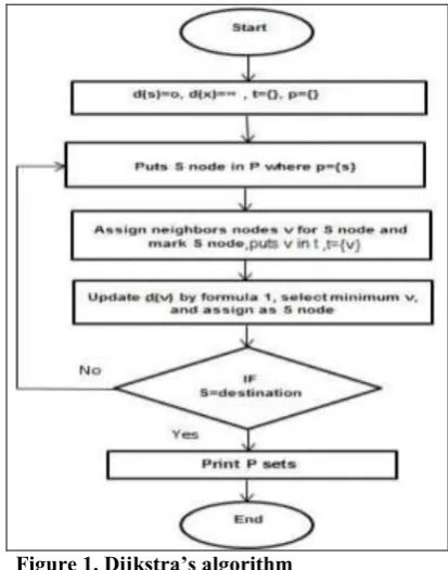
Conceived by Dutch computer scientist Edsger Dijkstra in 1956 and published in 1959[9]. Dijkstra's algorithm is used in search graph algorithm for solve the single-source shortest path problem for a weighted graph with non-negative edge path costs, producing a shortest path tree [5]. This algorithm is often used in routing and as a subroutine in other graph algorithms. The Dijkstra’s Algorithm finds the shortest path between two nodes on a network by use the greedy strategy where an algorithm that always takes the best immediate solution when finding an answer. Greedy algorithms find the overall optimal solution for some optimization problems, but may find less-than-optimal solutions for some instances of other problems. In Dijkstra's algorithm firstly, no path is known. Dijkstra's algorithm divides the nodes into two subset groups: temporary set (t) and permanently set (p). Then this algorithm assigns the zero distance value to source node s, and label it as permanent [The state of node s is (0, p)], and Assign to the remaining nodes a distance value of (∞) and label them as temporary. [The state of every other node is (∞, t)]. At each iteration, updates its distance label, and puts the node into a permanently set as permanently labeled nodes p. The permanently labeled distance associated with each examined node is the shortest path distance from the source node to the destination node. The source node is node s and neighbor's nodes are v. At each iteration the node s is selected and marked, then update distance and label for each node. Selected nodes neighbors for node s and update distance values for these node v by formula the following.
Dv = min {dv, ds + (s,v)} (1)
During the above formula, if the labeled distance of node u plus the weight of link (s, v) is shorter than the labeled distance of node v, then the estimated shortest distance from the source node to node v is updated with a value equal to. The algorithm continues the node examination process and takes the next node as source node. The algorithm terminates when is reached to the destination. This is process is clearly in a Figure1.
The computational complexity of the implementation of the Dijkstra's algorithm big-O notation is where n = number of vertices [4]. Big-O notation is frequently used in the computer science and mathematics domain to describe an upper bound on the growth rate of the algorithm. [1]
Figure 1. Dijkstra’s algorithm
3.2.
Bellman-ford algorithm
shortened, and if so, replace the path to the node with the found path. Relax the edge with only 2 nodes starting from the source node; the E (1, 2) of cost 7, the cost of the source node plus 7 is less than infinity. So, we replace the cost of the node 2 d (2) = 7. As well the E (1, 6) of cost 6 which is also less than infinity, then d (6) = 6 as figure 3. So relax edges for 5 times since n are 6. The step 3, consider the path with 3 nodes and relax the edge E (1,3) through 1→2→3, relax E (1,4) through 1→2→4 or 1→6→4 etc. The step 4, consider the path with 4 nodes. Thus, the process will continue. Hence, the final step gives the shortest path between each node and the source node. Thus all edges are relaxed, checked the negative cost cycle, and the appropriate boolean value is returned. Hence it is called the single-source shortest path algorithm. Bellman–Ford runs in time O (V,E) time, where V and E are the number of vertices and edges respectively. [2]
Algorithm1. Bellman-Ford Figure 2.Representation step1
Figure 3. Presentation the steps from 2 to 5
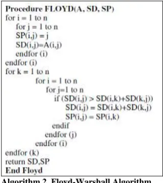
3.3 Floyd-Warshall Algorithm
Is an algorithm using to computing of the shortest paths between all pairs of vertices in a weighted graph with positive or negative edge weights. The Floyd– Warshall algorithm also known as Floyd's algorithm, Roy– Warshall algorithm, Roy–Floyd algorithm or the WFI algorithm [5]. The Floyd–Warshall algorithm was
published in its currently recognized form by Robert Floyd in 1962 [5]. Floyd-Warshall algorithm uses a matrix (n*n) of lengths as its input. This matrix represents lengths of all paths between nodes that do not contain any intermediate node is called distance matrix. If there is an edge between nodes i and j, than the matrix contains its length at the matrix. The diagonal of the matrix contains only zeros. If there is no edge between edges i and j, than the position (i,j) contains positive infinity [2]. This matrix recalculate at every iteration of the Floyd-Warshall algorithm. So, it's keep track of the shortest path between any two vertices, using only some subset of the entire collection of vertices as intermediate steps along the path. The matrix, which is created by the first iteration of the procedure, contains paths among all nodes using exactly one (predefined) intermediate node. Contain lengths using two predefined intermediate nodes. Finally the matrix uses n intermediate nodes. This process can be described using the following recurrent formula [2]:
(2)
The above formula is the heart of the Floyd–Warshall algorithm. The algorithm works by first computing shortest path (i, j, k) for all (i, j) pairs for k = 1, then k = 2, etc. This process continues until k = n, Then find the shortest path for all (i, j) pairs using any intermediate vertices. The pseudocode as shown in algorithm 2:
Algorithm 2. Floyd-Warshall Algorithm.
Otherwise, the value of the element in of j on the path from i to j. So we repeat this procedure, while the preceding node is not equal to i as Algorithm 2.1. The Floyd-Warshall algorithm runs in where N is number of nodes of the graph [1].
Algorithm 2.1 Floyed-warshall for finding the shortest path.
3.4. Johnson's algorithm
Is a way to find the shortest paths between all pairs of vertices in a graph, whose edges may have positive or negative weights? But no negative-weight cycles may exist. It combines the Bellman-Ford algorithm and Dijkstra’s algorithm to quickly find shortest paths. It is named after Donald B. Johnson, who first published the technique in 1977. The algorithm either returns (n*n) matrix of shortest-path weights for all pairs of vertices, or reports that the input graph contains a negative-weight cycle. The below algorithm is simply perform the actions for the Johnson's algorithm. Johnson's algorithm works as follows; firstly, produce s G' contains new vertex s with zero weight edges from it to all other nodes as algorithm 4. Then runs the Bellman-Ford algorithm on G' with source vertex s as line 2 at algorithm 4. The Bellman-Ford algorithm used to check for negative weight cycles. If this step detects a negative cycle, the algorithm reports the problem and terminated as line 3 at algorithms 4. Lines 4– 12 at algorithm 4 assume that G' contains no negative-weight cycles. Line 4-5 The bellman algorithm find the minimum weight h(v)=p(s,v) for each vertex v of a path from s to v. Line 6-7 compute the new weights by the formula following:
W'(u,v) = W(u,v) + h(u)-h(v) (2)
The for loop in line 9-12 compute the shortest paths weight p'(u,v) by using the Dijkstra's algorithm from vertex in v. Line 12 The correct shortest path stores in matrix as shown the formula 3.The final line is return the completed D matrix.
duv= P'(u,v) + h(u) – h(v) (3)
If we implement the min-priority queue in Dijkstra’s algorithm by a Fibonacci heap, Johnson’s algorithm runs in O (V2log V+VE) time. The simpler binary min-heap
implementation yields a running time of O (VE log V). [2]
Algorithm 3. Johnson’s Algorithm
3.5. Greedy best-first Search
Greedy best-first search3 tries to expand the node that is closest to the goal, on the: grounds that this is likely to lead to a solution quickly. Thus, it evaluates nodes by using just the heuristic function:
f (n) = h(n).
The straight line distance heuristic, which we will call hSLD. Greedy best-first search using hSLD finds a solution without ever expanding a node that is not on the solution path; hence, its search cost is minimal. The heuristic causes unnecessary nodes to be expanded. Furthermore, if we are not careful to detect repeated states, the solution will never be found. Greedy best-first search resembles depth-first search in the way it prefers to follow a single path all the way to the goal, but will back up when it hits a dead end. It is not optimal, and it is incomplete. The worst-case time and space complexity is O(bm), where m is the maximum depth of the search space.[7]
3.6.
A* search: Minimizing the total estimated
solution cost
The most widely-known form of best-first search is called A* search (pronounced "A-star search"). It evaluates nodes by combining g(n),the cost to reach the node, and h(n.),the cost to get from the node to the goal:
f(n) = g(n) + h(n) Since g(n) gives the path cost from the start node to node n, and h(n) is the estimated cost of the cheapest path from n to the goal, we have:
f(n) = estimated cost of the cheapest solution through n
h(n) satisfies certain conditions, A* search is both complete and optimal. The optimality of A* is straightforward to analyze if it is used with TREE-SEARCH. In this case, A* is optimal if h(n) is an admissible heuristic. A general proof that A* using TREE-SEARCH is optimal if h(n) is admissible. Suboptimal goal node G2 appears on the fringe, and let the cost of the optimal solution be C*.
Then, because G2 is suboptimal and because h(G2=) 0 (true for any goal node), we know
f (G2) = g(G2) + h(G2) = g(G2) > C* .
If h(n)does not overestimate the cost of completing the solution path, then we know that
f (n) = g(n) + h(n) <= C* .
Now we have shown that f (n) <= C* < f (G2) so G2 will not be expanded anti A* must return an optimal solution.
There are two ways to fix this problem. The first solution is to extend GRAPH-SEARCH so that it discards the more expensive of any two paths found to the same node. The second solution is to ensure that the optimal path to any repeated state is always the first one followed-as is the cfollowed-ase with uniform-cost search. A heuristic h(n)is consistent if, for every node n and every successor n' of n generated by any action a, the estimated cost of reaching the goal from n is no greater than the step cost of getting to n' plus the estimated cost of reaching the goal from n':
h(n)<= c(n,a , n') t h(nf).
A* is optimally efficient for any given heuristic function. That is, no other optimal algorithm is guaranteed to expand fewer nodes than A* (except possibly through tie-breaking among nodes with f (n) = C* A*'s main drawback. Because it keeps all generated nodes in memory (as do all GRAPH-SEARCH algorithms), A* usually runs out of space long before it runs out of time. For this reason, A* is not practical for many large-scale problems. Recently developed algorithms have overcome the space problem without sacrificing optimality or completeness, at a small cost in execution time. [5]
1. Pseudo code
(1) At initialization add the starting location to the open list and empty the closed list
(2) While there are still more possible next steps in the open list and we haven’t found the target:
(A) Select the most likely next step (based on both the heuristic and path costs)
(B) Remove it from the open list and add it to the closed (C) Consider each neighbor of the step. For each neighbor:
(i) Calculate the path cost of reaching the neighbor (ii) If the cost is less than the cost known for this location
then remove it from the open or closed lists (since we’ve now found a better route)
(iii) If the location isn’t in either the open or closed list then record the costs for the location and add it to the open list (this means it’ll be considered in the next search). Record how we got to this location. [6]
The loop ends when we either find a route to the destination or we run out of steps. If a route is found we
back track up the record of how we reached each location to determine the path. [6]
3.7. Memory-bounded heuristic search
The simplest way to reduce memory requirements for A* is to adapt the idea of iterative deepening to the heuristic search context, resulting in the iterative-deepening A* (IDA*) algorithm.
The main difference between IDA* and standard iterative deepening is that the cutoff used is the f-cost (g+ h) rather than the depth; at each iteration, the cutoff value is the smallest f -cost of any node that exceeded the cutoff on the previous iteration. Two more recent memory-bounded algorithms called RBFS and MA*.
Recursive best-first search (RBFS) is a simple recursive algorithm that attempts to mimic the operation of standard best-first search, but using only linear space. Its structure is similar to that of a recursive depth-first search, but rather than continuing indefinitely down the current path, it keeps track of the f-value of the best alternative path available from any ancestor of the current node. If the current node exceeds this limit, the recursion unwinds back to the alternative path. As the recursion unwinds, RBFS replaces the f -value of each node along the path with the best f -value of its children. In this way, RBFS remembers the f -value of the best leaf in the forgotten sub tree and can therefore decide whether it's worth re-expanding the sub tree at some later time. RBFS is somewhat more efficient than IDA*, but still suffers from excessive node regeneration. Like A*, RBFS is an optimal algorithm if the heuristic function h(n) is admissible. Its space complexity is linear in the depth of the deepest optimal solution, but its time complexity is rather difficult to characterize: it depends both on the accuracy of the heuristic function and on how often the best path changes as nodes are expanded.
IDA* and RBFS suffer from using too little memory. Between iterations, IDA* retains only a single number: the current f -cost limit. RBFS retains more information in memory, but it uses only linear space: even if more memory were available, RBFS has no way to make use of it.
Algorithm 4. Recursive Best First Search
3.8. Hill-climbing search
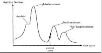
The hill-climbing search algorithm is shown in Figure 4. It is simply a loop that continually moves in the direction of increasing value-that is, uphill. It terminates when it reaches a "peak" where no neighbor has a higher value. Hill-climbing does not look ahead beyond the immediate neighbors of the current state.
Hill climbing is sometimes called greedy local search because it grabs a good neighbor state without thinking ahead about where to go next.
Local maxima: a local maximum is a peak that is higher than each of its neighboring states, but lower than the global maximum.
Ridges: Ridges result in a sequence of local maxima that is very difficult for greedy algorithms to navigate.
Plateaux: a plateau is an area of the state space landscape where the evaluation function is flat. It can be a flat local maximum, from which no uphill exit exists, or a shoulder. (1) Stochastic hill climbing: chooses at random from among the uphill moves; the probability of selection can vary with the steepness of the uphill move.
(2) First-choice hill climbing: implements stochastic hill climbing by generating successors randomly until one is generated that is better than the current state.
(3) Random-restart hill climbing: adopts the well-known adage, "If at first you don't succeed, try, and try again." It conducts a series of hill-climbing searches from randomly generated initial states, stopping when a goal is found. [7]
Figure 4. A one-dimensional state space landscape in which elevation corresponds to objective function. The aim is to find the global maximum. Hill-climbing search modifies the
current state to try to improve it, as shown by the arrow. The various topographic features are defined in the text.
Algorithm 5. Hill Climbing Search
3.9. Simulated annealing search
A hill-climbing algorithm that never makes "downhill" moves towards states with lower value (or higher cost) is guaranteed to be incomplete, because it can get stuck on a local maximum.
In contrast, a purely random walk-that is, moving to a successor chosen uniformly at random from the set of successors-is complete, but extremely inefficient. Simulated annealing is such an algorithm. In metallurgy, annealing is the process used to temper or harden metals and glass by heating them to a high temperature and then gradually cooling them, thus allowing the material to coalesce into a low-energy crystalline state. The simulated annealing solution is to start by shaking hard (i.e., at a high temperature) and then gradually reduce the intensity of the shaking (i.e., lower the temperature). Simulated annealing was first used extensively to solve VLSI layout problems in the early 1980s. It has been applied widely to factory scheduling and other large-scale optimization tasks. [7]
Algorithm 6. Simulated annealing search
3.10. Local beam search
halts. Otherwise, it selects the k best successors from the complete list and repeats.
In a local beam search, useful information is passed among the k parallel search threads. In its simplest form, local beam search can suffer from a lack of diversity among the k states-they can quickly become concentrated in a small region of the state space, making the search little more than an expensive version of hill climbing. A variant called stochastic beam search. Stochastic beam search chooses k successors at random, with the probability of choosing a given successor being an increasing function of its value. [5]
4
.
Related Work
In A* Search a technique from the field of Artificial Intelligence, is a goal-directed approach, i.e., it adds a sense of direction to the search process. For each vertex, a lower bound on the distance to the target is required. In each step of the search process, the node v is selected that minimizes the tentative distance from the source s plus the lower bound on the distance to the target t. The performance of the A* search depends on a good choice of the lower bounds. If the geographic coordinates of the nodes are given and we are interested in the shortest (and not in the fastest) path, the Euclidean distance from v to t can be used as lower bound. This leads to a simple, fast, and space-efficient method, which, however, gives only small speedups. It gets even worse if we want to compute fastest paths. Then, we have to use the Euclidean distance divided by the fastest speed possible on any road of the network as lower bound. Obviously, this is a very conservative estimation. Goldberg et al. Even report a slow-down of more than a factor of two in this case since the search space is not significantly reduced but a considerable overhead is added [6]. Shortest Path Algorithm is an important problem in graph theory, geographic information system, Path searching for road network and has applications in communications, transportation, finding shortest path in network and electronics problems. In graph theory, used many algorithm that solve the shortest path algorithms. [7]
5. Conclusion
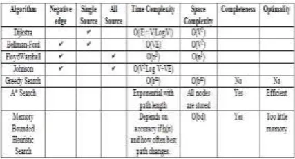
Shortest Path Algorithm is an important problem in graph theory and has applications in communications, transportation, and electronics problems. In graph theory, used many algorithm that solve the shortest path algorithms. Dijkstra’s algorithm finds solution in the single-pair, single-source, and single-destination shortest path problem. Johnsons’s algorithm identifies the solution in all pairs shortest path problem. The Floyd Warshall algorithm is assigned the shortest path between all pairs of vertices by a graph analysis algorithm. It's an example of dynamic programming. Bellman Ford algorithm obtains
solution in the single-source problem if the edge weights are negative too.
Tabel 1. Differences of Shortest Path Algorithm
References
[1] Anu Pradhan, and Kumar, G. 2013. "Finding All-Pairs Shortest Path for a Large-Scale Transportation Network Using Parallel Floyd-Warshall and Parallel Dijkstra Algorithm". Journal of Computing in Civil Engineering ASCE. 263-273.
[2] Hanaa M. Abu-Ryash, Dr.Abdelfatah A. Tamimi Department of Computer Science Faculty of Science and Information technology, Al-Zaytoonah University of Jordan, "Comparison Studies for Different Shortest path Algorithms", International Journal of Computer & Technology, May 29, 2015, pp. 5979-5986
[3] Mr. Girish P Potdar, Dr. R C Thool "Optimal Solution for Shortest Path Problem Using Heuristic Search Technique", International Journal of Advanced Research in Computer Engineering & Technology (IJARCET) Volume 3 Issue 9, September 2014, pp. 3247-3256
[4] Nizami Gasilov, Mustafa Doğan, and Volkan Arici. 2011. "Two-stage Shortest Path Algorithm for Solving Optimal Obstacle Avoidance Problem" JOURNAL OF RESEARCH (IETE). VOL 57. ISSUE 3, 278-185.
[5] Peter Hofner, and Bernhard Moller. 2012." Dijkstra, Floyd and Warshall meet Kleene". Formal Aspects of Computing, 459–476.
[6] Shrawan Kr. Sharma, B.L.Pal, " Shortest Path Searching for Road Network using A* Algorithm
[7] Stuart Russell, Peter Norving, Artificial Intelligence A Modern Approach, Second Edition
[8] Tom Lenaerts,"Artifical intelligenence 1: informed search" SWITCH, Vlaams Interuniversitair Instittuut voor Biotechnologies, Vrije Universiteit Brussel.