Improved Backpropagation Algorithms by Exploiting Data
Redundancy in Limited-Angle Diffraction Tomography
Pavel Roy Paladhi1, *, Ashoke Sinha2, Amin Tayebi1, Lalita Udpa1, and Satish Udpa1
Abstract—Filtered backpropagation (FBPP) is a well-known technique used in Diffraction Tomography (DT). For accurate reconstruction of a complex-valued image using FBPP, full 360◦ angular coverage is necessary. However, it has been shown that by exploiting inherent redundancies in the projection data, accurate reconstruction is possible with 270◦ coverage. This is called the minimal-scan angle range. This is done by applying weighting functions (or filters) on projection data of the object to eliminate the redundancies. There could be many general weight functions. These are all equivalent at 270◦ coverage but would perform differently at lower angular coverages and in presence of noise. This paper presents a generalized mathematical framework to generate weight functions for exploiting data redundancy. Further, a comparative analysis of different filters when angular coverage is lower than minimal-scan angle of 270◦ is presented. Simulation studies have been done to find optimum weight filters for sub-minimal angular coverage. The optimum weights generate images comparable to a full 360◦ coverage FBPP reconstruction. Performance of the filters in the presence of noise is also analyzed. These fast and deterministic algorithms are capable of correctly reconstructing complex valued images even at angular coverage of 200◦ while still under the FBPP regime.
1. INTRODUCTION
Diffraction tomography (DT) is a popular imaging modality [1, 2] used in a variety of applications such as medical imaging, non-destructive evaluation of materials, structural health monitoring, geophysics etc. [3, 4]. In the domain of optical imaging, this method has been explored in depth viz. optical diffraction tomography (ODT) with multi-disciplinary applications [5–7]. DT is a broad imaging technique of which ultrasound and microwave tomographic imaging are sub-classes. It is a comprehensive way of characterizing the complex valued object-function of the test object. The scheme is applicable to microwave tomography of tissue samples. It has been of great interest in tomography of human breast to identify malignant tumours [8–14]. The high contrast between healthy and cancerous breast tissue provides opportunities for clearly identifying malignancies within breast tissue. The contrast is much higher than in case of X-rays and hence microwave tomography is advantageous both in terms of true detection and radiation damage from X-rays. Further applications are in fields of SAR imaging. Various backprojection techniques have been explored for use in radar imaging and modified for better reconstructions [15–17]. Faster implementations for backprojections algorithms are also being intensely explored, e.g., [17]. Again, radar based methods have been combined with microwave tomography to generate higher resolutions for medical imaging [10]. Thus, any improvement in the traditional backpropagation techniques is of potential interest across multiple disciplines. This paper shows an approach to improve direct FBPP reconstruction of complex-valued objects at lower angular coverages than traditional requirements.
Received 2 December 2015, Accepted 9 February 2016, Scheduled 9 February 2016
* Corresponding author: Pavel Roy Paladhi ([email protected]).
1 Department of Electrical and Computer Engineering, Michigan State University, 428 S Shaw Lane, Rm-2120, East Lansing, Michigan
In the presence of weak scatterers, assuming the Born or Rytov approximations [2], the Fourier Diffraction Projection theorem (FDP) is applied. The FDP relates the scattered field data from the Region of Interest (ROI) to the 2D-Fourier Space of the ROI. Devaney developed the filtered backpropagation (FBPP) algorithm for this configuration to reconstruct a low-pass filtered image of the object function [1]. The traditional backpropagation technique requires projection data from [0, 2π] angular coverage for accurate image reconstruction of a complex image. Even though the formulation applies to weak scatterers, it has found a number of applications and since its introduction, a steady research focus has been maintained to increase the extent of usage for backpropagation-like algorithms for DT and making them more general in applicability, e.g., [18, 19]. A major challenge in many real world situations is that projection measurements cannot be gathered over full 360◦ view around the test object. With limited access to the object and decrease in angular coverage, the available data in the Fourier space decreases. Reconstruction from this partial Fourier space data leads to many artifacts and loss of important image features. Hence alternate schemes are needed for image reconstruction from limited angular coverage projection data. For highly sparse data or limited angular access various minimization, regularization, estimation techniques and statistical approaches are being successfully explored to make the reconstruction algorithms more robust to sparse and noisy data, e.g., [20, 21]. However, generally these are iterative methods and the total computation time depends on the convergence rate of the algorithm. A single step method would be always quicker provided it can handle the limited availability of data. In [23–26], a novel alternative approach for moderately limited angular access was introduced. It was shown that using inherent redundancies in the projection data from the conventional setup, exact reconstruction is possible with data from [0, 3π/2] coverage. For lower angular coverages, the algorithm results in significant distortions. In this paper we explore a technique that efficiently uses the redundancies in the Fourier space data from the conventional setup [27]. This technique can reconstruct better images (than regular FBPP) effectively over any range between π to 3π/2. This is a crucial development, as the demands on angular access for complex valued object reconstruction is lowered considerably. This paper proposes to use projection datasets optimally to get enhanced reconstructions from lower angular coverages. Also, this is a direct reconstruction method which does not employ any error minimization algorithms and hence is faster and accurate over angular coverages between 180◦–270◦.
The paper is organized as follows: Section 2 gives a short background of the FDP and FBPP algorithms and explains the minimal-scan complete dataset proposed in [23] and how equivalent systems of backpropagation algorithms can be generated. Section 3 introduces methods to generate weight function classes of backpropagation algorithms which can give better reconstruction than regular FBPP in the angular coverage range where the redundancy can still be exploited, i.e., between 180◦–270◦. Section 4 presents results from different backpropagation classes and analyses the relative performances at angular coverages below 270◦.
2. FBPP & THE MINIMAL SCAN REQUIREMENT IN DT
The fundamental theory underlying 2D-DT is the FDP. This relates the scattered field data from the Region of Interest (ROI) due to incident plane waves to the 2D-Fourier space of the ROI [2]. The traditional 2D-configuration is shown in Fig. 1. Let the object o(x, y) be illuminated with a monochromatic plane wave of frequency ν0. Let the wave be incident at an angleφ to the horizontal axis. Then, the 1D Fourier Transform (FT) of the scattered field measured along the straight lineη=l in the co-ordinate system (ξ, η) gives the values of the 2D transform of the object O(νx, νy) along a semi-circular arc in the frequency domain. As shown in the right half of Fig. 1, this arc will be tilted at an angle φ. The scattered field data and the object function are related by the following equation:
U(ν, l) = j 2ν2
0 −ν2 ej
√ ν2
0−ν2lO
ν,
ν02−ν2−ν0
, (1)
where U(ν, l) represents 1D FT of the scattered field, u(ξ, η) under Born approximation (measured at line η=l), andν lies in the range [−ν0,ν0].
(a) (b)
Figure 1. (a) Classical scan configuration of 2D DT and (b) relation of scattered field data with the 2D Fourier space of the objective function.
as presented in [23], the backpropagation integral takes the form:
a(r, θ) = 2π
φ=0 ν0
νm=−ν0
ν0
ν |νm|M(νm, φ)·e
[j2πνmcos(φ−α−θ)]
dνmdφ (2)
In Eq. (2),a(r, θ) is the objective function being reconstructed in polar spatial coordinates (r,θ), ν0 the frequency of the incident monochromatic plane wave andφbeing the incidence angle,M(νm, φ)
a modified 1D FT of the scattered data, defined as
M(νm, φ) =U(νm, φ) jν
2π2ν2 0
e−j2πνl, (3a)
whereν=ν02−νm2,νa= sgn(νm)
ν2
m−νμ2,νμ=j(ν−ν0) and
α = sgn(νm) arcsin
1 2ν0
ν2
m−νμ2
, (3b)
Without loss of generality, α could be further simplified to
α= 1 2arcsin
νm
ν0
. (3c)
In order to reconstruct a complex object accurately, a full knowledge of M(νm, φ) in the range [0, 2π]
is necessary to perform the integration in Eq. (2), [22].
2.1. Minimal Scan FBPP
(a) (b)
(d) (c)
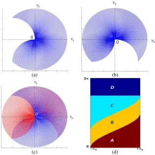
Figure 2. (a) Fourier space coverage for 270◦ angular access by segment OB in Fig. 1(b) same for segmentOA of Fig. 1. (c) Superposition of the two coverages from (a) and (b). (d) The Fourier data-space in alternate co-ordinate system with angular coverage along y-axis and the wave number along x-axis.
projection and stacking them up on top of each other sequentially. In this layout, the entire Fourier dataspace can be divided into four sub-regionsA,B,C and D as shown in Fig. 2(d). The boundaries for the four regions can be expressed asA= [|νm| ≤ν0,0≤φ <2α+π/2], B= [|νm| ≤ν0, π/2 + 2α≤
φ <2α+π], C= [|νm| ≤ν0, π+ 2α≤φ <3π/2] andD= [|νm| ≤ν0,3π/2≤φ <2π]. As seen in (2c),
α is a function of νm and so the regions have nonlinear boundaries.
From FDP theorem the following periodicity holds [24]:
M(νm, φ) =M(−νm, φ+π−2α) (4)
This also implies that for every point in regionA (orB), there is a point of identical value in regionC (orD). Thus, the knowledge ofM(νm, φ) in regionsAandB, makes information inCandDredundant.
This redundancy can be handled by normalizing the dataspace using appropriate weight filters. The weighted dataset M(νm, φ) can be defined as M(νm, φ) =w(νm, φ)M(νm, φ), where w(νm, φ) satisfies
the condition
w(νm, φ) +w(−νm, φ+π−2α) = 1. (5)
It should be noted that since region D is unavailable in a 270◦ coverage we setw(νm, φ) = 0 in region
D and correspondingly w(νm, φ) = 1 in region B. For regions A and C, any weight functions are
valid as long as they satisfy Eq. (5). Using the weighted dataset M(νm, φ) we can apply the regular
backpropagation algorithm for reconstruction. This is called Minimal-Scan Filtered Backpropagation (MS-FBPP) which involves evaluating the following integral
aW(r, θ) = 1 2
3π/2
φ=0 ν0
νm=−ν0
ν0 ν|νm|M
(ν
This integral can, in theory, exactly reconstruct an image from a 270◦ angular coverage by utilizing data redundancy in projection data. The weights w(νm, φ) can then be used to define classes of
backpropagation algorithms for image reconstruction. An example of weight functions introduced in [23] is given in equation below:
w(νm, φ) = ⎧ ⎪ ⎪ ⎪ ⎪ ⎪ ⎪ ⎨ ⎪ ⎪ ⎪ ⎪ ⎪ ⎪ ⎩ sin2 π 4 · φ π/4 +α
, inA,
1, inB,
sin2
π 4 ·
3π/2−φ π/4−α
, inC,
0, inD.
(7)
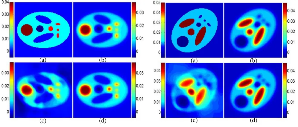
This will be used as a reference later on in Section 4 for comparison with the weight functions that are proposed in this paper. The filter of Eq. (7) will be referred to as sine-squared filter in this paper. This is a very elegant and simple filter designed to have continuity across the boundaries between regionsA,B, C and D. To demonstrate the efficacy of MS-FBPP, a sample reconstruction is performed on a Shepp-Logan type phantom with complex parameter distribution. The real part of the phantom is shown in Fig. 3(a) and the imaginary part in Fig. 4(a). Reconstruction from regular FBPP and MS-FBPP using weights of (7) are given in Fig. 3 and Fig. 4. The images show the MS-FBPP algorithms capable of generating accurate reconstructions from 270◦ (equivalent to full coverage), whereas the regular FBPP image shows considerable distortion at 270◦.
Weight filters which are discontinuous across boundaries of the four regions in Fig. 2(d) can give rise to artifacts, especially in the case of discrete data. Further, for each class of weights, its distribution in frequency space of Fig. 2(d) also determines the performance when the available coverage is below 270◦. This is because,C andDare complementary to regionsAandB respectively. An efficient weight function set would be that which spans most of the regionsA and B, thus limiting the requirement to access regions C and D. In effect such weights can generate good reconstructions even from angular coverages below 270◦. The next section explains a systematic approach to generate general classes of weight functions.
(a) (b)
(d) (c)
Figure 3. Demonstration of the MS-FBPP concept, (a) real part of original image, (b) FBPP reconstruction from 360◦ coverage, (c) FBPP reconstruction from 270◦ coverage and (d) MS-FBPP reconstruction from 270◦ coverage.
(a) (b)
(c) (d)
3. GENERATION OF EFFICIENT WEIGHT FUNCTIONS
From previous section, we see that the weights in regionsB andDare 1 and 0 respectively. Notice that weights in regionCcan be generated from weights of regionA, because for any point (νm, φ) in regionC, the point (−νm, φ+π−2α) inAis equivalent due to (4), and we getw(νm, φ) = 1−w(−νm, φ+π−2α), using Eq. (5). Thus it is sufficient to generate weights for the regionA only.
Furthermore from Eq. (5), the non-negative weights are bounded above by 1. So in region A, for any fixed νm, the functionw(νm,·) =:F(·) is defined on [0,2α+π/2], and takes values between 0 and
1. However it is desirable to have weights which are continuous at the boundaries between two regions. Weights which are discontinuous at the boundaries will generate artifacts in case of discrete datasets as noticed in [23].
Here we propose an approach to generate the weights, by using cumulative distribution functions (cdf) to modelF(·), which are guaranteed to be bounded within 0 and 1. To obtain continuous weights, we use continuousF with
F(0) = 0, and F(2α+π/2) = 1. (8)
This will ensure that weights are continuous at the boundary between regionsAandB, and consequently at the boundaries between regions B and C, and C and D. This approach would allow us to choose weights from a no. of cdfs. In this article, we primarily use beta-cdf to generate weights. The standard beta-cdf is defined as:
F(x|a, b) = x
−∞f(t|a, b)dt. (9)
wherea >0,b >0, andf is the standard beta probability density function:
f(t|a, b) = ⎧ ⎨ ⎩
1 B(a, b)t
a−1(1−
t)b−1, 0≤t≤1,
0, otherwise,
(10)
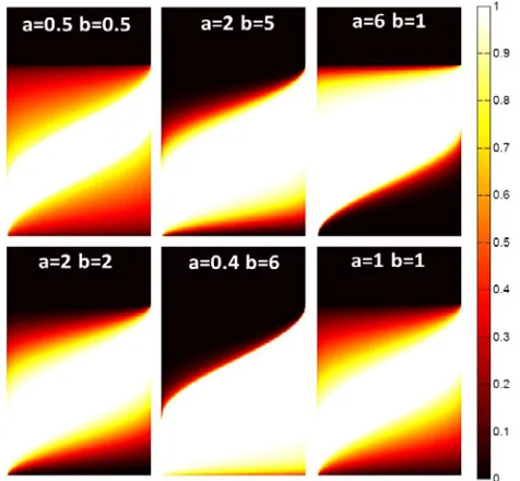
and B(a, b) = 01ta−1(1−t)b−1dt. We obtain a family of beta-cdf’s by changing values of a and b in Eq. (10), as shown in Fig. 5. Notice that the standard beta-cdf has support [0, 1], while in regionA
Figure 5. Beta-cdf plots for different values of the parameters aand b.
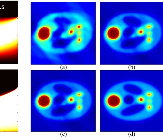
for a fixed νm, we need to define weights for φ ∈ [0,2α+π/2]. This can be achieved by substituting x= 2α+φπ/2 in Eq. (9). The corresponding weight profiles in the frequency domain are shown in Fig. 6. The plots in Fig. 5 can be used to understand how the weights will be distributed in RegionsAand C. Fig. 6 gives useful insight on choosing optimal parameter values. For example, with combinations a= 2, b= 5 ora= 6, b= 1, region Ais not well covered, whereas for a= 0.4, b= 6, region A has been almost fully covered with near unity weights leaving Region C with mostly near-zero weights. This combination is expected to better utilize data redundancy than the other combinations shown in Fig. 5. This can be further illustrated through Fig. 7 and Fig. 8. Fig. 7 shows some weight distributions in the Fourier space (in the alternative co-ordinate system). The beta-cdf parameters used to generate these weights are shown in inset white text. Fig. 8 shows the reconstructed real parts of the images by using these weights. Reconstruction was performed from sub-minimal angular coverage of 200◦. The weights which cover regionAmore completely also give better reconstructions. It should be noted that especially for coverages lower than 270◦, we receive less information from C, hence an optimum weight function should span most of regionAwith near unit weightage. Since the weights are continuous across the boundaries of the regions, the transition from zero to unity should be adequate to retain as much information as possible within region A but also not too abrupt to minimize generation of artifacts in case of discrete datasets. In this paper the authors demonstrate the efficacy of using cdf based weights in image reconstruction at sub-minimal angular coverage. To do this, good parameter values were heuristically determined in the following manner: for the beta-cdf, a parametric sweep over the range of a ∈ [0.2,3], b ∈ [1,6] was performed and the corresponding weight distributions were generated. Reconstructions were performed with these weights for a sub-minimal coverage of 200◦. The weight combination which gave the least distortion in the reconstruction and maintained highest correlation with the original image was chosen as the optimum set. Within this range, the parameter combination a= 0.4,b= 6 gave best results and is used for image reconstruction in the next section.
Similar approach can be used to generate weight functions from other cumulative distribution functions as well, for instance with the gamma-cdf. However, since the gamma distribution has
(a) (b)
(c) (d)
Figure 7. Images showing weight distributions in Fourier domain generated by parametric variation of the beta-cdf. The parameters a and b used for each weight distribution are inset in each plot. Frequency is plotted along abscissa and angular coverage along ordinate.
(a) (b)
(c) (d)
unbounded support, a suitable transformation of the argument is required to ensure that the weights are constructed with continuity properties at the boundaries as discussed above. Details about constructing the weights with gamma-cdf are described in the Appendix. For this case, the parameters were varied in the range a ∈ [0.1,3.1], b ∈ [0.1,3.1]. The best parameter set found from this range was a = 2.1, b= 0.1. In this paper, results from beta and gamma distributions using these optimum parameters for each distribution will be presented and compared with the results from weights given in Eq. (7).
4. RESULTS
This paper presents results from simulated projection data for DT valid under the Born approximation. The test image is complex. Both the real and imaginary parts of the image are, in effect, modified versions of the Shepp-Logan phantom, a standard model used to validate computed tomography algorithms. The real and imaginary parts of the test image are shown in Figs. 3(a) and 4(a). The projection data from the phantom was computed following [23, 24]. The image matrix is 128×128 pixels with pixel size of λ/8. The image has an area of 16λ×16λ. The objective of this paper was to define a procedure to generate optimum weights which can exploit the redundancy for angular coverages below 270◦ and up to 180◦, where redundancy is still present in the projection data.
4.1. Noiseless Reconstruction
Proceeding in the manner described in the previous section to generate weights, the following optimum parameters for different cdfs were used: for beta-cdf, a= 0.4, b= 6; for gamma-cdf, a= 2.1,b = 0.1. Reconstructed images have been plotted from regular FBPP and MS-FBPP using different weight functions for coverages 270◦ and 200◦ (an example of sub-minimal angular coverage). Both real and imaginary parts are shown in Figs. 9 and 10 respectively. The reconstructions show the beta-cdf and gamma-cdf based weights generate a very stable reconstruction even in lower angular coverage of 200◦, with beta-cdf performing slightly better overall.
To compare the performance of different MS-FBPP algorithms quantitatively, we use their Mean-Absolute-Error (MAE) with respect to the original image. The MAE is calculated as the absolute mean pixel-by-pixel difference between the original and reconstructed image: MAE = n1 |imgorig(i)− imgrecon(i)|, where imgorig(i) is the ith pixel in the original image and imgrecon(i), the ith pixel in the reconstructed image andnis the total number of pixels in the image. The errors in real and imaginary parts of image were calculated separately. At 200◦ coverage, for the real part of the image, the beta-cdf based reconstruction had a 30.77% lower error than regular FBPP, while the gamma-cdf based reconstruction yielded a 29.11% lower error. A similar trend is seen for the imaginary part of the image. The sine-squared based weights give accurate reconstructions at 270◦, but below 270◦ they progressively deteriorate. These are clearly not optimum choices for coverage<270◦. For example, at 200◦ coverage, the quality of reconstruction degrades for both the regular FBPP and sine-squared weighted FBPP. However, the latter has a higher error than the regular FBPP reconstruction (2.46% higher in real part of image). A more detailed error-analysis has been done with noisy data in the next subsection. Below 180◦ coverage, the redundancy disappears and using weights alone, in principle cannot produce a better reconstruction than regular FBPP. So, reconstructed images are not shown for further lower coverage. However, it should be noted that for these lower coverages, reconstruction from un-optimized weights will generate higher errors than regular FBPP. This is also evident from the sine-squared weights based reconstructions for sub-minimal coverages. The optimized cdf based weights perform much better than both the sine-squared weights and regular FBPP.
4.2. Reconstruction with Noisy Data
(a) (b)
(c) (d)
(e) (f)
(g) (h)
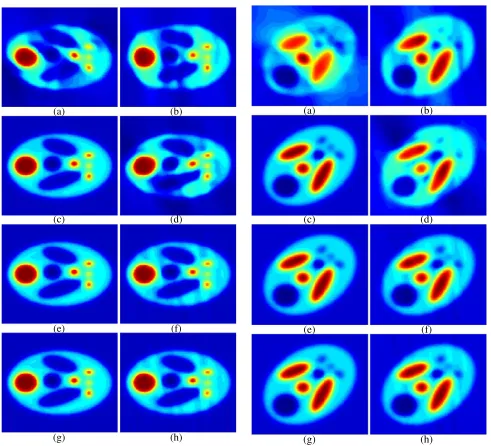
Figure 9. Reconstructed real part from complex test image under noiseless conditions. The left column shows reconstruction from 270◦ coverage and right column shows reconstruction from 200◦ coverage. (a), (b) using regular FBPP, (c), (d) using sine-sq weights, (e), (f) using gamma-cdf weights, (g), (h) using beta-cdf weights.
(a) (b)
(c) (d)
(e) (f)
(g) (h)
Figure 10. Reconstructed imaginary part of the test image under noiseless conditions. The left column shows reconstruction from 270◦ coverage and right column shows reconstruction from 200◦ coverage. (a), (b) using regular FBPP, (c), (d) using sine-sq weights, (e), (f) using gamma-cdf weights, (g), (h) using beta-cdf weights.
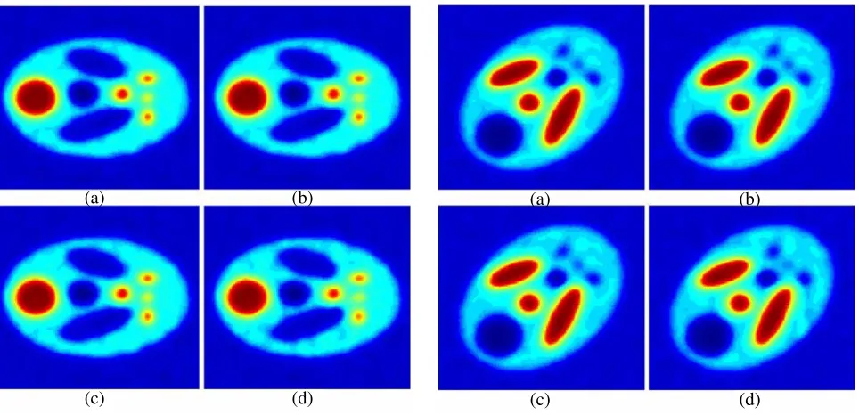
(a) (b)
(c) (d)
Figure 11. Reconstruction of real part of image from 3 dB awgn projection data using beta-cdf weights for angular coverages, (a) 270◦, (b) 250◦, (c) 220◦, (d) 200◦.
(a) (b)
(c) (d)
Figure 12. Reconstruction of imaginary part of image from 3 dB awgn projection data using beta-cdf weights for angular coverages, (a) 270◦, (b) 250◦, (c) 220◦, (d) 200◦.
Figure 13. MAE calculated at different coverages for real part of reconstructed image with regular FBPP and MS-FBPP using different weights.
Figure 14. MAE calculated likewise Fig. 13 for imaginary part of reconstructed image.
weights based on beta-cdf with a= 0.4, b= 6, which earlier gave best results with noiseless data. The reconstructions show robustness of the algorithm to noise levels that could be reasonably expected from good experimental data.
Figure 11 and Fig. 12 show that the beta-cdf based weights are capable of maintaining all the features and without any artifacts up to 220◦. The reconstruction at 200◦ is also almost distortionless. The responses are stable and the images are not affected noticeably due to the noise injection as seen in these figures.
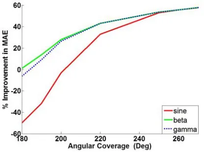
Figure 15. Percentage improvement of MAE from different weights over regular FBPP at different coverages for real part of reconstructed image.
Figure 16. Percentage improvement of MAE likewise Fig. 15 for imaginary part of recon-structed image.
weights are able to generate MAEs which remain lower than regular FBPP and are very steady up to 200◦. For the beta-cdf based reconstruction, as the coverage decreases from 270◦ to 200◦, the value of MAE increases by only 2.33% in the real part and 1.45% in the imaginary part of the image. For gamma-cdf based reconstruction, the numbers are 4.31% and 2.64% respectively. For coverages below 200◦, as the redundancy is lost, these two MAEs increase and slowly converge towards the MAE of a regular FBPP reconstruction around 180◦. For the sine-squared based weights, the MAEs are almost equal to the other two weights in the interval [250◦, 270◦], but rapidly increases as the coverage reduces, and become greater than the regular FBPP and other two MS-FBPP reconstructions. At 200◦coverage, the MAE of the real part of the image increases by as much as 46.05% of its value at 270◦ coverage and that of the imaginary part by 48.62%.
The MAE plots for the regular FBPP algorithm in Fig. 13 and Fig. 14 may be counterintuitive at the first look. This is because the error increases as the angular coverage increases from 180◦ to 270◦. However, it should be noted that starting from 180◦ coverage and above, there are regions in the Fourier space where there is overlap from the two halves OA and OB of the semi-circular arc AOB in Fig. 1. The regular FBPP doesn’t apply weights to the dataspace to account for these partial overlaps and hence gives higher errors in reconstruction. At 360◦ coverage, as there is complete coverage by both the arcs OA and OB, weighting the dataspace is not required. Following this, it is found that error increases from 180◦ coverage to a maximum at 270◦, where there is maximum asymmetry with respect to overlapping coverages in Fourier space by the two half semi-circles,OA and OB. Weighting becomes most important at 270◦. Beyond that, the importance decreases again and vanishes at 360◦ coverage. For this reason, an error increase is seen between 180◦ and 270◦ coverage. The solution to this problem in that coverage range is to weight the projection dataspace appropriately before applying the backpropagation algorithm.
5. CONCLUSION
In this paper, a new approach to exploit data redundancy within the traditional 2D DT setup has been explored. Using cumulative distribution functions, especially the beta-cdf, it was shown that distortionless reconstructions of complex-valued object functions are possible even at angular coverage of 200◦. The advantages of this observation are numerous. The major benefit is that it reduces the angular scanning requirements for accurate reconstructions. This also implies shorter access times for collecting relevant projection data. In medical applications, this can mean a lower amount of exposure to the interrogating energy and also, fewer artifacts due to temporal variations caused by movements of the patient. For still lower coverages (<180◦), the redundancy in the tomographic dataset vanishes and alternate approaches such as total variation (TV) minimization, compressed sensing, etc. are explored for application to DT setups. Combining these techniques with MS-FBPP could be a scope of future research work. In this paper, results have been validated through simulated data in the case of plane wave excitation but can be extended to the fanbeam geometry as well. This is also of significance to medical imaging. Studies with fanbeam geometry and the performance of these algorithms with real experimental data will be explored in the future work of this study.
APPENDIX A. GAMMA-CDF BASED WEIGHT GENERATION
The gamma-cdf is defined as F(x) = −∞x f(t)dt, where f is the gamma probability density function defined as:
f(t|a, b) = ⎧ ⎨ ⎩
1 Γ(a)bat
a−1
e−t/b, t≥0,
0, t <0.
(A1)
where a >0 andb > 0 are parameters, and Γ(a) = 0∞ta−1e−tdt is standard gamma-function. As we can see, gamma-cdf has support on [0, ∞), F(2α+π/2)<1, which does not meet Eq. (9). Therefore, weights created using gamma-cdf in its original form will be discontinuous at the boundary betweenA and B, and consequently at the boundary between B and C. One possible way to get a continuous weight is by inputting a transformed argument. So for fixed νm ∈[−ν0, ν0], we shall construct weights
by using
w(νm, φ) =F
tan
π 2
φ 2α+π/2
, (A2)
whereF is the gamma-cdf as defined above.
REFERENCES
1. Devaney, A., “A filtered backpropagation algorithm for diffraction tomography,” Ultrasonic Imaging, Vol. 4, No. 4, 336–350, 1982.
2. Kak, A. C. and M. Slaney, “Tomographic imaging with diffracting sources,” Principles of Computerized Tomographic Imaging, IEEE Press, New York, 1988.
3. Semenov, S., “Microwave tomography: Review of the progress towards clinical applications,” Phil. Trans. of the Royal Society A: Mathematical, Physical and Engineering Sciences, Vol. 367, No. 1900, 3021–3042, 2009.
4. Ritzwoller, M. H., et al., “Global surface wave diffraction tomography,” Jour. of Geophys. Res. Solid Earth, Vol. 107, No. B12, ESE 4-1–ESE 4-13, 2002.
5. Gorski, W. and W. Osten, “Tomographic imaging of photonic crystal fibers,”Optics Letters, Vol. 32, No. 14, 1977–1979, 2006.
6. Sung, Y., et al., “Optical diffraction tomography for high resolution live cell imaging,”Opt. Express, Vol. 17, No. 1, 266–277, 2009.
7. Kostencka, J., et al., “Accurate approach to capillary-supported optical diffraction tomography,”
8. Catapano, I., L. Di Donato, L. Crocco, O. M. Bucci, A. F. Morabito, T. Isernia, and R. Massa, “On quantitative microwave tomography of female breast,”Progress In Electromagnetics Research, Vol. 97, 75–93, 2009.
9. Drogoudis, D. G., G. A. Kyriacou, and J. N. Sahalos, “Microwave tomography employing an adjoint network based sensitivity matrix,” Progress In Electromagnetics Research, Vol. 94, 213–242, 2009. 10. Baran, A., D. J. Kurrant, A. Zakaria, E. C. Fear, and J. LoVetri, “Breast imaging using microwave tomography with radar-based tissue-regions estimation,” Progress In Electromagnetics Research, Vol. 149, 161–171, 2014.
11. Bayat, N. and P. Mojabi, “The effect of antenna incident field distribution on microwave tomography reconstruction,”Progress In Electromagnetics Research, Vol. 145, 153–161, 2014. 12. Tayebi, A., et al., “Design and development of an electrically-controlled beam steering mirror for
microwave tomography,” AIP Conf. Proc. QNDE, Vol. 1650, No. 1, 501–508, 2015.
13. Tayebi, A., et al., “Dynamic beam shaping using a dual-band electronically tunable reflectarray antenna,” IEEE Trans. on Antennas and Propagation, Vol. 63, No. 10, 4534–4539, 2015.
14. Paladhi, P. R., et al., “Reconstruction algorithm for limited-angle diffraction tomography for microwave NDE,” AIP Conf. Proc. QNDE, Vol. 1581, No. 1, 1544–1551, 2014.
15. Ren, X. Z., et al., “A three-dimensional imaging algorithm for tomography SAR,” IEEE International Geoscience and Remote Sensing Symposium 2009, 184–187, Cape Town, South Africa, 2009.
16. Ren, X.-Z., L. H. Qiao, and Y. Qin, “A three-dimensional imaging algorithm for tomography SAR based on improved interpolated array transform,”Progress In Electromagnetics Research, Vol. 120, 181–193, 2011.
17. Capozzoli, A., C. Curcio, and A. Liseno, “Fast GPU-based interpolation for SAR backprojection,”
Progress In Electromagnetics Research, Vol. 133, 259–283, 2013.
18. Tsihrintzis, G. A. and A. J. Devaney, “Higher-order (nonlinear) diffraction tomography: Reconstruction algorithms and computer simulation,” IEEE Trans. Image Proc., Vol. 9, No. 9, 1560–1572, 2000.
19. Vouldis, A. T., et al., “Three-dimensional diffraction tomography using filtered backpropagation and multiple illumination planes,”IEEE Trans. Instr. and Meas., Vol. 55, No. 6, 1975–1984, 2006. 20. Ayasso, H., et al., “Bayesian inversion for optical diffraction tomography,” Jour. Modern. Optics,
Vol. 57, No. 9, 765–776, 2010.
21. Sung, Y. and R. R. Dasari, “Deterministic regularization of three-dimensional optical diffraction tomography,”JOSA A, Vol. 28, No. 8, 1554–1561, 2011.
22. Devaney, A., “The limited-view problem in diffraction tomography,” Inverse Problems, Vol. 5, No. 4, 501–521, 1989.
23. Pan, A. and M. A. Anastasio, “Minimal-scan filtered backpropagation algorithms for diffraction tomography,”JOSA A, Vol. 16, No. 12, 2896–2903, 1999.
24. Pan, X., “Unified reconstruction theory for diffraction tomography, with consideration of noise control,” JOSA A, Vol. 15, No. 9, 2312–2326, 1998.
25. Anastasio, M. A. and X. Pan, “Full-and minimal-scan reconstruction algorithms for fan-beam diffraction tomography,” Applied Optics, Vol. 40, No. 20, 3334–3345, 2001.
26. Pan, X. and M. A. Anastasio, “On a limited-view reconstruction problem in diffraction tomography,”IEEE Trans. Med. Imag., Vol. 21, No. 4, 413–416, 2002.
27. Paladhi, P. R., et al., “Data redundancy in diffraction tomography,” 31st International Review of Progress in Applied Computational Electromagnetics (ACES), Vol. 31, No. 4, 1–2, 2015.
28. Tsihrintzis, G. A. and A. J. Devaney, “Stochastic diffraction tomography: Theory and computer simulation,”Signal Processing, Vol. 30, No. 1, 49–64, 1993.