Scholarship@Western
Scholarship@Western
Electronic Thesis and Dissertation Repository
8-23-2018 1:30 PM
Development of image-based surgical planning software for
Development of image-based surgical planning software for
bone-conduction implants
conduction implants
Carlos D. Salgado
The University of Western Ontario
Supervisor Ladak, Hanif M.
The University of Western Ontario Agrawal, Sumit K.
The University of Western Ontario
Graduate Program in Electrical and Computer Engineering
A thesis submitted in partial fulfillment of the requirements for the degree in Master of Engineering Science
© Carlos D. Salgado 2018
Follow this and additional works at: https://ir.lib.uwo.ca/etd
Part of the Biomedical Commons, and the Biomedical Devices and Instrumentation Commons
Recommended Citation Recommended Citation
Salgado, Carlos D., "Development of image-based surgical planning software for bone-conduction implants" (2018). Electronic Thesis and Dissertation Repository. 5535.
https://ir.lib.uwo.ca/etd/5535
This Dissertation/Thesis is brought to you for free and open access by Scholarship@Western. It has been accepted for inclusion in Electronic Thesis and Dissertation Repository by an authorized administrator of
i
The BONEBRIDGE bone-conduction device is used to treat conductive and mixed hearing losses. The size of its floating mass transducer (FMT) can preclude implantation in certain anatomies, necessitating comprehensive surgical planning. Current techniques are time consuming and difficult to transfer to the operating room. The objective of this thesis was to develop software for calculating skull thickness to the dura mater to find locations for the FMT and to the first air cells which guarantee sufficient bone for the implant screws to grasp. Temporal bone computed tomography (CT) images were segmented and processed and custom Matlab code was written to generate and test thickness colormaps. For validation, measurements performed by a trained otologist were compared to the algorithm estimations achieving sub-millimeter accuracy. Results suggest this software can be used in the surgical workflow to automate thickness estimation and aid in finding an ideal location for the BONEBRIDGE device and screws.
Keywords
ii
Co-Authorship Statement
Chapter 2 consists of a manuscript that has been submitted to and is currently under review by the Journal of Otolaryngology – Head & Neck Surgery:
Salgado CD, Rohani SA, Ladak HM, Agrawal SK. Development and validation of a surgical planning tool for bone-conduction implants. J Otolaryngol Head Neck Surg, submitted July 2018.
iii
Dedication
A mi familia
Por ser los mejores ejemplos de superación, por enseñarme de perseverancia. Por su amor y apoyo incondicional y por mantenerse tan cerca aún en la distancia.
A mi amor
Por ser mi fuente de inspiración para crecer y ser mi mejor version. Por motivarme a cumplir mi aspiración y apoyarme tanto sin condición.
A mis amigos
A los se han quedado, a los que llegaron en el camino y me echaron la mano. A los que con una charla me motivaron, los reconozco a todos como mis hermanos.
iv
Acknowledgments
I would first like to thank Dr. Hanif Ladak and Dr. Sumit Agrawal, my research co-supervisors, for their patient guidance, enthusiastic encouragement and useful critiques of this research work. I extend special thanks to Dr. Ladak for taking me in and for his mentorship. My grateful thanks are also extended to Dr. S. Alireza Rohani for his help through the duration of the study.
I wish to thank Robert W. Koch, John E. Iyaniwura, Daniel Allen, Brad Gare and Lauren Siegel, members of the auditory biophysics laboratory, who were happy to lend a helping hand and made the lab a pleasant environment.
I gratefully acknowledge the funding received towards my Master’s from the Science and
Technology Council of Mexico (Consejo Nacional de Ciencia y Tecnología, CONACYT) that has sponsored this research.
v
Table of Contents
Abstract ... i
Co-Authorship Statement... ii
Dedication ... iii
Acknowledgments... iv
Table of Contents ... v
List of Tables ... vii
List of Figures ... viii
List of Abbreviations ... x
Chapter 1 ... 1
Introduction ... 1
1.1 Overview ... 1
1.2 The Human Hearing System ... 1
1.3 The Temporal Bone ... 3
1.4 Hearing Loss ... 4
1.4.1 Types and Degrees of Hearing Loss ... 5
1.4.2 Treatment of Hearing Loss ... 6
1.5 Bone Conduction Devices... 6
1.6 The BONEBRIDGE... 8
1.6.1 Implant Surgery ... 10
1.6.2 Computed Tomography ... 11
1.6.3 Surgical Planning ... 14
1.7 Image segmentation ... 14
1.8 Literature Review... 15
1.9 Objective ... 16
vi
References ... 18
Chapter 2 ... 21
Development and Validation ... 21
2.1 Background ... 21
2.2 Methods... 24
2.2.1 Clinical CT images ... 24
2.2.2 Algorithm Development ... 24
2.2.3 Validation ... 26
2.3 Results ... 28
2.3.1 Algorithm ... 28
2.3.2 Validation ... 29
2.4 Discussion ... 35
2.5 Conclusion ... 37
References ... 38
Chapter 3 ... 40
Conclusions and Future Work ... 40
3.1 Contribution ... 40
3.2 Limitations and Future Work ... 41
3.2.1 Additional Testing ... 41
3.2.2 Decision Support ... 41
3.2.3 Porting ... 42
References ... 43
vii
List of Tables
Table 1-1: Hearing loss categorized by the degree of loss ... 5
Table 1-2: Reference intensity values in the Hounsfield Scale ... 13
viii
List of Figures
Figure 1-1: Coronal cross-section of ear anatomy. ... 1
Figure 1-2: Middle and inner ear anatomy. ... 2
Figure 1-3: Location of the temporal bone in the skull ... 3
Figure 1-4: Location of the two parietal bones (red) in the skull. ... 4
Figure 1-5: The BONEBRIDGE, its components and dimensions... 8
Figure 1-6: Locations for BONEBRIDGE implant. ... 10
Figure 1-7: The BCI lifts... 11
Figure 1-8: Axial slice view of a head CT scan. ... 12
Figure 1-9: Sample head CT scan. ... 13
Figure 1-10: Segmentation results ... 15
Figure 1-11: Representation of an axial slice view of a segmentation ... 16
Figure 2-1: Cross-section of an implanted BONEBRIDGE ... 22
Figure 2-2: Schematic illustrating the ray casting algorithm to the first air cell and to dura . 25 Figure 2-3: Thickness color maps from bone to air cells ... 26
Figure 2-4: Grid of evenly distributed points laid by the program ... 27
Figure 2-5: Thickness color map from bone to air cell ... 29
Figure 2-6: Scatter-plot of measurements from bone to air cell by the algorithm and expert. 30 Figure 2-7: Box-plot of algorithm and expert measurements to the first air cell. ... 31
Figure 2-8: Scatter-plot of measurements from bone to dura by the algorithm and expert .... 32
ix
x
List of Abbreviations
2D Two-Dimensional
3D Three-Dimensional
BAHA Bone-Anchored Hearing Aid
BC Bone Conduction
BCD Bone Conduction Device
CHL Conductive Hearing Loss
CI Confidence intervals
CT Computed Tomography
dB HL Decibels of Hearing Loss
FMT Floating Mass Transducer
HU Hounsfield Units
MAD Mean Absolute Difference
MHL Mixed Hearing Loss
PTA Pure Tone Average
SNHL Sensorineural Hearing Loss
SSD Single Sided Deafness
Chapter 1
Introduction
1.1
Overview
In this thesis, patient data were analyzed for bone conduction implant surgery, an implant designed to alleviate hearing loss. A method was then developed to automate a part of the surgical planning procedure, with the goal of saving clinical time. This introductory chapter begins with a short review on the anatomy and physiology of the ear, followed by an explanation of the degrees and types of hearing loss, current bone conduction devices, and lastly summarizes the image processing approaches adopted in this research.
1.2
The Human Hearing System
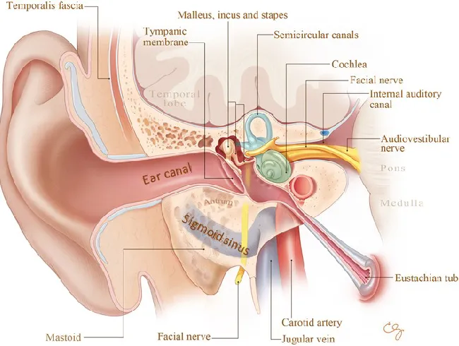
The human ear is divided into three sections. External, middle and internal. An overview of the human ear anatomy can be observed in Figure 1-1.
The external ear is formed by the auricle and ear canal. It receives sound waves travelling through the air in the ear canal and conducts them into the middle ear.
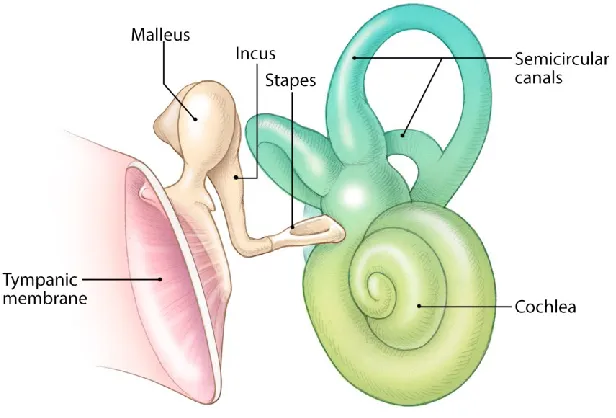
The middle ear consists of the tympanic membrane and the internal bones that form the ossicular chain (incus, malleus and stapes). The sound waves in the ear canal vibrate the tympanic membrane, which in turn triggers the ossicular chain that sends the mechanical vibrations into the inner ear.
The inner ear consists of both the vestibular system, which is related to balance, and the cochlea and auditory nerve, which are related to hearing. Inside the cochlea, hair cells convert the received vibrations into electrical impulses of different frequencies that are then sent to the brain via the auditory nerve. Figure 1-2 depicts the main components of the middle and inner ears.
1.3
The Temporal Bone
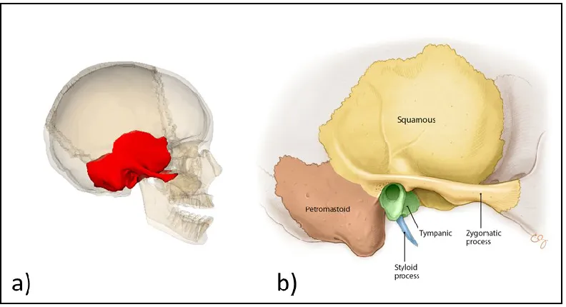
The human skull has two temporal bones, one on either side of the skull as shown in Figure 1-3a.
Figure 1-3: Location of the temporal bone in the skull (a) from [2] and its components (b) from [1]
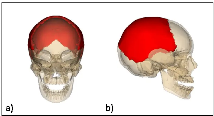
Figure 1-4: Location of the two parietal bones (red) in the skull. (a) Frontal and (b) lateral views from [3]
1.4
Hearing Loss
Hearing loss is a global public health concern recognized by the World Health
Organization (WHO). It is the second impairment, after anemia, that affects the greatest number of people around the globe [4]. Approximately 1.33 billion people endure hearing loss [4], of which 473 million people suffer from disabling hearing loss [5], making up 5% of the worldwide population. There are currently 34 million children suffering from disabling hearing loss where language skills and educational development require special attention and are often delayed if the impairment is left unattended, even when hearing loss is unilateral [6]. According to the WHO, 60% of childhood hearing loss is
disabling hearing loss, like with chronic ear infections, occupational noise and ototoxic medications are left unattended, the global statistic could rise to 630 million people by 2030 and to 900 million in 2050 [7], doubling the current occurrence up to 10% of the population. To prevent this, the WHO recommends early identification of the issue to prompt the use of hearing aids or implants to improve quality of life. It is estimated that 72 million people could potentially benefit from a hearing device [7], adding to the challenge of supplying sufficient access to physicians.
1.4.1 Types and Degrees of Hearing Loss
Hearing loss can be classified by type and degree. There are three main types of hearing loss. Conductive hearing loss (CHL) is the reduction of sound transmission in the middle or outer ear. CHL can be caused by a damaged or perforated tympanic membrane; abnormalities preventing the proper movement of the ossicular chain, such as fixed malleus syndrome [11]; or pathologies, such as otitis media or middle ear malformations [12] in the aforementioned structures; among other causes. Sensorineural hearing loss (SNHL) is caused by abnormalities in the inner ear, where speech recognition is often decreased. Mixed hearing loss (MHL) is a combination of problems in the outer, middle and inner ears, and shares elements from CHL and SNHL. Table 1-1 presents degrees of hearing loss in accordance with the American Speech-Language-Hearing Association; values are in decibels of hearing loss (dB HL) which measures the degree of hearing loss in relation to the standard of normal hearing.
Table 1-1: Hearing loss categorized by the degree of loss [13] Hearing Loss Degree Hearing Loss Range
(dB HL)
Normal Up to 15 Slight 16-25
1.4.2 Treatment of Hearing Loss
Various treatment options are available depending on the type (conductive, sensorineural, or mixed) and degree of hearing loss. Patients with mild to moderate hearing loss,
regardless of type, can largely benefit from wearing hearing aids. Hearing aids deliver amplified sound into the ear and do not require surgery.
Severe to profound hearing loss is most commonly sensorineural, and can be treated with a cochlear implant, which involves an electrode that is surgically implanted into a
patient’s cochlea. Cochlear implants deliver electrical impulses to the cochlear nerve, bypassing the outer and middle ear, in order to allow the patient to hear an array of frequencies that permit the interpretation of speech.
Conductive and mild MHL are typically treated with hearing aids. However, many patients cannot wear hearing aids due to previous surgery, recurrent infections, or atresia (where the external auditory canal and/or pinna are congenitally malformed). These patients can be treated with a bone conduction device (BCD), which bypass the external auditory canal and middle ear by transmitting sound vibrations through the temporal bone into the cochlea.
1.5
Bone Conduction Devices
Bone conduction is the transmission of sound through the bones of the skull, it occurs when the vibrations representing sound that normally happen in the middle ear take place in the skull instead. These vibrations compress and expand the skull forcing the
movement of the fluids in the cochlea. The intensity of the transmission depends on the incoming sound frequency and bone structure [14].
persistent drainage [15, 16]. BCDs are the only option to treat CHL when it is accompanied by bony atresia or intractable drainage [15].
Percutaneous devices were the first type of BCD developed during the 1970s out the necessity to improve on the discomforts of conventional hearing aids, such as auditory feedback and pressure [14]. The most commonly used device of this category is the Bone-Anchored Hearing Aid (BAHA), introduced in Sweden in the late 1970s [17]. The BAHA stimulates the temporal bone via an osseointegrated (adhered to bone) screw made of titanium and an abutment through the skin (percutaneous) connected to the external unit. After no longer being able to wear conventional hearing aids, patients have reported improvement in speech recognition, sound quality, and comfort with the BAHA [18]. Even though the complication rate for the BAHA is low, the percutaneous abutment and the interface with the titanium screw can represent risk of recurring infection, skin overgrowth, or wound dehiscence [16].
Passive transcutaneous BCDs avoid the issues related to the percutaneous nature of the BAHA by stimulating a magnet implanted transcutaneously through an external
stimulator, vibrating the bone through the skin instead of directly. However, it has been reported that in comparison with the BAHA, the hearing improvement at higher
frequencies is considerably lower, and the vibration in the soft tissue may cause a variety of skin problems such as swelling or infection after fitting [19]. A transcutaneous version of the BAHA was introduced in 2013 [20].
In active transcutaneous BCDs, vibrations are transmitted directly to the temporal bone via a floating mass transducer (FMT) that converts sound into vibrations. This active component is implanted in the bone under the skin. In contrast with the percutaneous BAHA, the electrical signal from the processor is transmitted through the skin instead of through mechanical vibrations [19]. Active transcutaneous BCDs have fewer
1.6
The BONEBRIDGE
The BONEBRIDGE is a partially implantable, active transcutaneous BCD developed by MED-EL (Innsbruck, Austria) that was first implanted in June 2011 as part of a clinical trial and was launched onto the European market in September 2012. The first
BONEBRIDGE implant in North America was performed at London Health Sciences Centre in April, 2013 [21, 22].
The device consists of a floating mass transducer (FMT) surgically implanted into the temporal bone, which is powered trancutaneously by a transmitter coil [16, 23] and a digital audio processor that is magnetically held in place by the aforementioned coil beneath the skin [24]. In addition to CHL and MHL, the BONEBRIDGE can in some cases treat severe-to-profound SNHL in one ear, also known as Single Sided Deafness (SSD) if the contralateral ear has normal hearing. The BONEBRIDGE device is displayed in Figure 1-5.
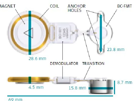
Figure 1-5: The BONEBRIDGE, its components and dimensions. Image courtesy of MED-EL [25]
As opposed to the BAHA, the two screws securing the device in the temporal bone do not need to be osseointegrated, therefore the BONEBRIDGE can be activated
osseointegration of screws with the BAHA have been shown to fail in some pediatric cases [26].
The BONEBRIDGE is indicated for patients who are aged 5 years and above, have conductive or mixed mild-to-moderate hearing loss and can still benefit from sound amplification. The main audiological requirement is that the pure tone average (PTA) bone conduction (BC) threshold measured at 0.5, 1, 2, 3 and 4 kHz should be better than or equal to 45 dB of hearing loss per ear. PTA refers to the average hearing threshold of a given set of frequencies. This parameter helps determine the degree of residual hearing the patient has and their capacity to interpret speech.
Individuals with any of the following conditions in their medical history may benefit from the BONEBRIDGE, being that they are unable to wear conventional hearing aids: revision tympanoplasty, ear canal stenosis or chronically draining ears, otosclerosis or tympanosclerosis that cannot be rectified by surgery, or congenital malformations where ear canals are absent and cannot be restored through conventional surgery. The screening process to determine candidacy for the BONEBRIDGE also involves checking for sudden deafness, acoustic neuroma, or other conditions which cause severe to profound sensorineural hearing loss on one side [14].
The BONEBRIDGE was developed to improve the audiological outcomes associated with passive transcutaneous BCDs and to reduce the complications associated with percutaneous BCDs. A recent systematic review of 29 studies, of which 12 studied safety, found that implant-related complications occurred in only 6 out of 117 patients, where minor adverse events such as headaches and wound pain were experienced and only one case required superficial revision surgery [14]. Other events included postoperative wound pain and dizziness, temporary tinnitus, headache, vertigo, seroma, and skin infection. Another study by Lassaletta et al. evaluated 27 postoperative BONEBRIDGE patients using pain questionnaires and found no significant postoperative pain
1.6.1 Implant Surgery
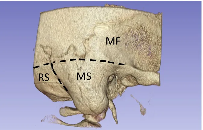
The implant surgery for the BONEBRIDGE consists of drilling a bed in the temporal bone which allows for the placement of the FMT in accordance with the implant’s
dimensions. There are currently three surgical approaches described in the literature and each is performed depending on a patient’s specific anatomy. The transmastoid approach is the most common approach for cases with previous middle ear surgeries with normal anatomy and is dependent on the volume of the mastoid. The venous sinuses and the dura mater are least likely to be compromised in this approach. The retrosigmoid approach is indicated for patients with difficult mastoid anatomy and is ideal for patients who have undergone previous mastoidectomy for chronic otitis media. However, the bone in this region is often curved, and surgery requires dissection of the nuchal musculature. The middle fossa approach may also be used as an alternative to the transmastoid approach. In this approach, the incision is located above the ear in the squamous temporal bone and is approximately 3 cm in length (comparatively smaller than in the other two
approaches), and cosmetically hidden in the hairline. Since the bone in this area can be thin, dura may be exposed; however there is minimal risk or sequelae [28, 29].
Approximate locations for the mentioned approaches are displayed in Figure 1-6.
In difficult cases, compression of the sigmoid sinus or dura can appear unavoidable, but it can be minimized by using BCI lifts. The BCI lifts are washers ranging in size from 1 to 4 mm and can be attached to the BONEBRIDGE FMT to allow it to fit difficult
anatomies [14]. Figure 1-7 showcases the BCI lifts.
Figure 1-7: The BCI lifts , from 1 to 4 mm in size, aid in the implantation of the BONEBRIDGE in difficult anatomies. Image courtesy of MED-EL [25]
1.6.2 Computed Tomography
Computed tomography (CT) is an imaging modality capable of generating cross-sectional images (slices) by using X-rays taken from different angles of the target anatomy. CT images are displayed in grayscale representing the intensity of the light absorbed by the observed tissue. Head CT scans are typically used to detect head injury, where the darker structures indicate less tissue density and brighter structures indicate denser tissue. A head CT scan is employed in determining if a patient’s anatomy is appropriate for the
placement of the BONEBRIDGE implant. CT allows for good visualization of
Figure 1-8: Axial slice view of a head CT scan. Only one slice of a sequence of slices is shown. Image courtesy of 3D Slicer [31, 32]
CT datasets consist of stacks of multiple two-dimensional (2D) slice images of the same specimen. Figure 1-9a represents a stack of axial head CT slices forming a 3D dataset. Slice data can be displayed in three-dimensional (3D) environments using medical image visualization software such as the open-source 3D Slicer software (www.slicer.org) [31, 32]. Figure 1-9b demonstrates the 3D rendering of the same dataset.
In CT, gray level intensities are described by the Hounsfield scale. The values in the scale are related to the linear attenuation coefficient of tissues and are expressed in
non-dimensional units, called Hounsfield units (HU) or CT numbers, that are determined by the following formula:
𝐻𝑈 = [μ𝑚𝑎𝑡𝑒𝑟𝑖𝑎𝑙−μ𝑤𝑎𝑡𝑒𝑟
Figure 1-9: Sample head CT scan. (a) Representation as a stack of 2D slices forming a (b) 3D Rendering of the same dataset. Image courtesy of 3D Slicer [31, 32]
where μ𝑤𝑎𝑡𝑒𝑟 tends to zero and is the linear coefficient of water. Medical grade CT scanners are calibrated with water as the reference. Table 1-2 lists HU values for
common biological materials. The Hounsfield scale is used in image analysis applications to locate the boundaries of a material within an image with a known HU number.
Table 1-2: Reference intensity values in the Hounsfield Scale [33–36]
Substance HU
Air -1000
Lung -600 to -700
Fat -50
Water 0
Blood +13 to +75
Muscle +50
Brain 0 to +100
D4 Bone (Fine
trabecular bone) +150 to +350 D3 Bone (Porous
trabecular bone)
+350 to +850
D2 Bone (Thick porous cortical bone)
+850 to +1250
D1 Bone (Dense cortical bone)
1.6.3 Surgical Planning
For BONEBRIDGE implantation, the patient’s anatomy is analyzed by visualizing the
bony anatomical structures to determine if it allows for appropriate placement of the FMT implant. Specifically, the region of the skull that is selected must be thick enough to fully house the implant.
Manually finding a suitable location is achieved by performing a CT scan of the patient’s
head and navigating through the axial orientation CT slices to try to find a suitable location for the FMT based on the distance to the dura mater (the outer layer of
membrane protecting the brain). It is essential that during this procedure, the anatomy is analyzed to avoid the risk of injury to important anatomical structures, including the chorda tympani [37], the sigmoid sinus or the facial nerve [38] during implantation [39];
or significant modification of the temporal bone pneumatisation (the air cell1 system) that
could affect the middle ear pressure buffers [40].
Manually determining the most suitable location to implant the FMT is time consuming and hinders the surgical workflow, which is why surgeons have expressed a need for quick and intuitive skull thickness estimation tools. A few attempts have been made to develop algorithms to estimate the thickness of the skull from each patient’s CT scan and
generate a map that can visually guide the surgeon in selecting a location that is thick enough to house the implant.
1.7
Image segmentation
Segmentation is an image processing technique used to partition a digital image to simplify its analysis. Image segmentation is employed in medical imaging to separate anatomical structures for visualization and diagnosis. Thresholding is the simplest form of segmentation, where an HU number is used as the lower grayscale intensity boundary to binarize an image into two values: pixels with HU equal to or above the threshold
1Air cells in bone are cavities filled by air. Air cells are present in human temporal bones. The air cells
represent pixels inside the segmentation (assuming the region of interest is brighter than other tissue) and HU values below the threshold are considered outside the segmentation. The opposite applies if the threshold is set as an upper boundary (i.e., the tissue of
interest is darker than the other tissue). Figure 1-10 shows the segmentation result when using a lower threshold value of 150 HU, therefore labelling all pixels within the data with intensities 150 HU and above as the segmented part. Because the thinner type of bone is described as having a CT number of 150 HU, the figure displays the skull within the dataset.
Figure 1-10: Segmentation results (BELOW) and 3D model (ABOVE) of sample data using 150 HU threshold to segment bone.
1.8
Literature Review
To improve on slice-by-slice manual processing to find a suitable implant location, some surgeons have reported using volume rendering of the BONEBRIDGE FMT inside CT images of the head, and simultaneously navigating through axial slices to determine a location with sufficient space to house the implant [14]. A common tool used for this approach is the BB FASTVIEW (CEIT, Guipuzcoa, Spain) software. The only guidance
to find the location for the implant are the anatomical landmarks and the patient’s clinical
for screw placement as described below. Also, processing times have been reported to be over an hour long [41].
Other approaches overlay color maps on temporal bone models using different colors to depict the thickness of the bone from the cortical layer, but with no consideration of the air cells of the skull [42, 43]. This is problematic as the inclusion of the air cells in the segmentation can lead to over-estimation of the bone thickness, which may result in surgical complications if an implant location where there is not enough bone to hold the surgical screws is selected. Figure 1-11 represents a fictional case where the
segmentation would prevent the visualization of the air cells, and the implant (overlaid) would be placed in an area without enough thick bone to hold it. Improper placement of the implant can result in secretory otitis media, among other complications such as cholesteatoma [40]. The software developed for this approach was presented as a C++ application with much quicker run rimes than the BB FASTVIEW approach, but it is not available to the public for download [42].
Figure 1-11: Representation of an axial slice view of a segmentation where air cells are considered bone (LEFT). Example of implant location where there is not enough
bone to hold the BONEBRIDGE’s surgical screws (RIGHT)
1.9
Objective
to the dura mater, therefore aiding in the surgical planning of the BONEBRIDGE FMT, as well as the placement of the screws. The second objective was to validate the tool by
comparing a sample of the algorithm’s thickness estimations to measurements made by a
surgeon with BONEBRIDGE implantation experience.
1.10
Hypothesis
References
1. Jackler R, Gralapp C. Stanford medicine otolaryngology head & neck surgery otologic surgery atlas. 2017. http://med.stanford.edu/sm/ohns-otologic-surgery-atlas/. Accessed 5 May 2018.
2. Temporal bone. 2009.
https://commons.wikimedia.org/wiki/category:temporal_bone#/media/file:tempor al_bone.png. Accessed 21 Jun 2018.
3. File:Parietal bone.png. 2009.
https://commons.wikimedia.org/w/index.php?search=parietal+bone&title=special: search&go=go&searchtoken=494y0e3lxsj5ayf27zfynbaxp#/media/file:parietal_b one.png. Accessed 27 Jun 2018.
4. Vos T, Allen C, Arora M, Barber RM, Brown A, Carter A, et al. Global, regional, and national incidence, prevalence, and years lived with disability for 310 diseases and injuries, 1990–2015: a systematic analysis for the global burden of disease study 2015. Lancet. 2016;388:1545–602.
5. Wilson BS, Tucci DL, Merson MH, O’Donoghue GM. Global hearing health care: new
findings and perspectives. Lancet. 2017;390:2503–15.
6. Lieu JEC. Speech-language and educational consequences of unilateral hearing loss in children. Arch Otolaryngol Head Neck Surg. 2004;130:524–30.
7. WHO. 10 Facts about deafness. 2018.
http://www.who.int/features/factfiles/deafness/en/. Accessed 24 May 2018. 8. WHO. Deafness and hearing loss. 2018.
http://www.who.int/en/news-room/fact-sheets/detail/deafness-and-hearing-loss. Accessed 24 May 2018.
9. Feder K, Michaud D, Ramage-morin P, Mcnamee J, Beauregard Y. Prevalence of
hearing loss among Canadians aged 20 to 79 : Audiometric results from the 2012 /
2013 Canadian health measures survey. 2015;26:18–25.
10. Gregory MC, Atkins CL, Barker DF. WHO - Hearing loss due to recreational exposure to loud sounds. N Engl J Med. 2015;330:714.
11. Stenfelt S, Goode RL. Bone-conducted sound: Physiological and clinical aspects. Otol Neurotol. 2005;26:1245–61.
12. Siegert R, Kanderske J. A new semi-implantable transcutaneous bone conduction device: Clinical, surgical, and audiologic outcomes in patients with congenital ear canal atresia. Otol Neurotol. 2013;34:927–34.
13. Clark J. G. Uses and abuses of hearing loss. J Am speech-langauge-hearing Assoc. 1981;23 January:493–500.
14. Sprinzl GM, Wolf-Magele A. The BONEBRIDGE bone conduction hearing implant: indication criteria, surgery and a systematic review of the literature. Clin
Otolaryngol. 2016;41:131–43.
16. Gerdes T, Salcher RB, Schwab B, Lenarz T, Maier H. Comparison of audiological results between a transcutaneous and a percutaneous bone conduction instrument in conductive hearing loss. Otol Neurotol. 2016;37:685–91.
17. Lustig LR, Arts HA, Brackmann DE, Francis HF, Molony T, Megerian CA, et al. Hearing rehabilitation using the BAHA bone-anchored hearing aid: Results in 40 patients. Otol Neurotol. 2001;22:328–34.
18. Mylanus EAM, Snik AFM, Cremers C. Patients opinions of bone anchored vs conventional hearing aids. Arch Otolaryngol Head Neck Surg. 1995;121:421–5. 19. Reinfeldt S, Hakansson B, Taghavi H, Eeg-Olofsson M. New developments in
bone-conduction hearing implants: A review. Med Devices Evid Res. 2015;8:79–93.
20. Gawęcki W, Stieler OM, Balcerowiak A, Komar D, Gibasiewicz R, Karlik M, et al.
Surgical, functional and audiological evaluation of new BAHA Attract system implantations. Eur Arch Oto-Rhino-Laryngology. 2016;273:3123–30.
21. Bone implant gives new hope to hearing impaired. 2013. https://www.ctvnews.ca/sci-tech/bone-implant-gives-new-hope-to-hearing-impaired-1.1277726. Accessed 21 Jul 2018.
22. LHSC first in North America to perform BONEBRIDGE bone conduction implant. 2013.
http://www.lhsc.on.ca/About_Us/LHSC/Publications/Homepage/BONEBRIDGE. htm. Accessed 21 Jul 2018.
23. Sprinzl G, Lenarz T, Ernst A, Hagen R, Wolf-Magele A, Mojallal H, et al. First European multicenter results with a new transcutaneous bone conduction hearing implant system: Short-term safety and efficacy. Otol Neurotol. 2013;34:1076–83. 24. Lassaletta L, Sanchez-Cuadrado I, Muñoz E, Gavilan J. Retrosigmoid implantation of
an active bone conduction stimulator in a patient with chronic otitis media. Auris Nasus Larynx. 2014;41:84–7.
25. MED-EL Image Gallery. http://www.medel.com/image-gallery/. Accessed 5 May 2018.
26. Christensen L, Richter GT, Dornhoffer JL. Update on bone-anchored hearing aids for pediatric patients with profound unilateral HL. Arch Otolaryngol Head Neck Surg. 2010;136:175–7.
27. Lassaletta L, Calvino M, Zernotti M, Gavilán J. Postoperative pain in patients undergoing a transcutaneous active bone conduction implant (BONEBRIDGE). Eur Arch Oto-Rhino-Laryngology. 2016;273:4103–10.
28. Zernotti ME, Sarasty AB. Active Bone Conduction Prosthesis : BONEBRIDGE TM. Int Arch Otorhinolaryngol. 2015;19:343–8.
29. Weiss BG, Bertlich M, Scheele R, Canis M, Jakob M, Sohns JM, et al. Systematic radiographic evaluation of three potential implantation sites for a
30. Güldner C, Heinrichs J, Weiß R, Zimmermann AP, Dassinger B, Bien S, et al. Visualisation of the BONEBRIDGE by means of CT and CBCT. Eur J Med Res. 2013;18:1–6.
31. 3D Slicer. http://www.slicer.org/. Accessed 13 Jul 2018.
32. Fedorov A, Beichel R, Kalphaty-Cramer J, Finet J, Fillion-Robbin J-C, Pujol S, et al. 3D slicers as an image computing platform for the quantitative imaging network. Magn Reson Imaging. 2012;30:1323–41.
33. Chugh T, Jain AK, Jaiswal RK, Mehrotra P, Mehrotra R. Bone density and its importance in orthodontics. Journal of Oral Biology and Craniofacial Research. 2013;3:92–7.
34. Hebb AO, Poliakov A V. Imaging of deep brain stimulation leads using extended hounsfield unit CT. Stereotact Funct Neurosurg. 2009;87:155–60.
35. Kazerooni EA, Gross BH. Cardiopulmonary Imaging. Lippincott Williams & Wilkins; 2004.
36. Hounsfield, G. N. Computerized transverse axial scanning (tomography): Part 1. Description of system. Br J Radiol. 1973;46:1016-22.
37. Gopalan P, Kumar M, Gupta D, Phillipps JJ. A study of chorda tympani nerve injury and related symptoms following middle-ear surgery. J Laryngol Otol.
2005;119:189–92.
38. Fayad JN, Wanna GB, Micheletto JN, Parisier SC. Facial nerve paralysis following cochlear implant surgery. Laryngoscope. 2003;113:1344–6.
39. Law EKC, Bhatia KSS, Tsang WSS, Tong MCF, Shi L. Head and neck CT pre-operative planning of a new semi-implantable bone conduction hearing device. Eur Radiol. 2016;1686–95.
40. Cinamon U, Sadé J. Mastoid and Tympanic Membrane as Pressure Buffers: A quantitative study in a middle ear cleft model. Otol Neurotol. 2003;24:839–42. 41. Kong TH, Park YA, Seo YJ. Image-guided implantation of the BONEBRIDGE TM
with a surgical navigation : A feasibility study. Int J Surg Case Rep. 2017;30:112–
7.
42. Barakchieva MM, Wimmer W, Dubach P, Arnold AM, Caversaccio M, Gerber N. Surgical planning tool for BONEBRIDGE implantation using topographic bone thickness maps. Int J Comput Assist Radiol Surg. 2015;10:97–8.
43. Wimmer W, Gerber N, Guignard J, Dubach P, Kompis M, Weber S, et al.
Chapter 2
Development and Validation
of a Surgical Planning
Tool for Bone-Conduction Implants
2.1
Background
The BONEBRIDGE® (Med-El GmbH, Innsbruck, Austria) is a transcutaneous bone-conduction device (BCD) intended to treat conductive (CHL) and mixed hearing losses (MHL). The device consists of an externally worn audio processor and a subcutaneous floating mass transducer (FMT) implant that is surgically anchored to the temporal bone [1]. The external component powers the FMT, classifying the BONEBRIDGE as an active, semi-implantable BCD [2]. The active nature of the FMT avoids the transfer of vibrational energy transcutaneously, thus overcoming the shortcomings of percutaneous and passive transcutaneous bone conduction devices [3, 4].
One disadvantage of the BONEBRIDGE is that the FMT is 8.7mm in height and 15.8mm in diameter, therefore surgical planning is required in order to find safe locations for implantation. Currently described locations include the mastoid, retrosigmoid, and middle fossa areas [5]. In the mastoid, there can often be limited room between the sigmoid
sinus, tegmen mastoideum2, external auditory canal, and facial nerve to safely house the
implant. This location is often excluded in patients with chronic otitis media or previous mastoidectomies [4]. The retrosigmoid and middle fossa areas are alternatives in these cases, however the skull thickness can often preclude complete implantation without dural compression and/or the use of BCI lifts [5–9]. In addition, the screws securing the implant typically require 3-4 mm of cortical bone thickness for fixation, however in
highly pneumatized temporal bones, the cortex adjacent to the air cells can be very thin. An implanted BONEBRIDGE is shown in Figure 2-1.
Figure 2-1: Cross-section of an implanted BONEBRIDGE bone-conduction device [10]
Current surgical planning techniques use computed tomography (CT) images to perform manual thickness measurements [10]. As these are conducted on two dimensional slices, the eventual location is difficult to transfer to the patient in the operating room. Some research groups such as Zernotti [5] and Weiss et al. [7] have experimented with the BB FASTVIEW tool (Center for Technical Studies and Research at the University of Navarra, Spain) which allows visualization of the FMT inside CT slices and three-dimensional (3D) reconstructions. In their work, they described three potential
Plontke [12] proposed a similar planning tool that implemented 3D visualization with AMIRA (Thermo Fisher Scientific, Waltham, MA, USA), however this commercial tool is costly and not readily available to surgeons for pre-operative planning. This technique also required manually moving the virtual implant to determine the optimal location, with no automated guidance for the surgeon.
Treece et al. [13, 14] developed a technique to calculate the cortical thickness in cadaveric femurs. This method consisted of thresholding to find an initial approximate surface, then fitting the surface to the data by comparing the intensity values on the cortical layer. Next, a new surface was interpolated and its vertices and normals were used to guide the thickness calculation, which was solved with a generic curve fitting algorithm that found the local image minima. This algorithm estimated the cortical thickness for each surface vertex, yielding approximately 17,000 thickness estimates per sample. Lillie et al. adapted this algorithm to measure cranial vault cortical thickness, which was found to be below 4 mm on average in multiple areas of the skull [15, 16].
Wimmer et al. [17] described a different technique to measure the thickness of the temporal bone for the surgical planning of bone-conduction implants. This method incorporated thresholding, cropping, manual editing, and then morphological filtering to find the inner and outer surfaces of the bone. The thickness was estimated by calculating the Euclidean distance (straight-line distance) between their vertices. This generated a distance from the cortical bone to the dura, however the air cells were not considered as they had been filled via a morphological hole filter. The last iteration of this group’s
technique, described by Barakchieva et al. [18], was developed using the C++ programming language.
2.2
Methods
2.2.1 Clinical CT images
Twelve cadaveric temporal bone CT images were obtained using a Discovery CT750 HD Clinical Scanner (GE Healthcare, Chicago, IL). The scanner was set to acquire images at a resolution of 234 µm, a slice thickness of 0.625 mm, and an x-ray voltage of 120 kV. Ethics approval was obtained through Western University’s Committee for Cadaveric
Use in Research (approval number #19062014). The data used in the current study are available from the corresponding author upon request.
2.2.2 Algorithm Development
2.2.2.1 Segmentation
To prototype the algorithm, the images were first processed using the open source software 3D Slicer (www.slicer.org). The region of interest (ROI) contained the entire temporal bone, including the mastoid, retrosigmoid, and middle fossa areas.
Segmentation was then performed utilizing a thresholding filter to separate bone from surrounding soft tissues. Depending on the case, dilation was used to add single layers of voxels to the nearest eight integers; a connectivity filter was used to remove regions smaller than 400 voxels not connected to the enclosed segmentation, and the
morphological remove islands filter was used to remove regions partly connected to the segmentation smaller than 200 voxels. This ensured the final segmentations were closed surfaces. Lastly, the resulting closed surfaces were converted into models.
2.2.2.2 Post-Processing
The segmented models were exported to Geomagic (3D Systems, Morrisville, North Carolina, USA) for smoothing and averaging. This was done to reduce the number of triangles in the surface mesh, thereby preventing long computation times. The
2.2.2.3 Ray Casting
A custom program was written in Matlab (MathWorks, Natick, Massachusetts, USA) to implement a traversal ray casting algorithm, adopted from Amanatides and Woo [19], on the segmented models. The primary parameters of the algorithm were the voxel intensity thresholds of the cortical bone, air cells and the dura mater (Figure 2-2). The first two thresholds used in this experiment were selected in accordance with the Misch
classification of bone [20]. The threshold for bone was set to 600 Hounsfield units (HU), corresponding to thin cortical bone, and the threshold for air was set to 150 HU, below the fine trabecular bone intensity. These parameters were determined during development by visualizing the algorithm results on test images. HU values tested for thicknesses to air are displayed in Figure 2-3.
Figure 2-2: Schematic illustrating the ray casting algorithm to the first air cell and to dura
algorithm had actually found dura, and not a large air cell.
Figure 2-3: Thickness color maps from bone to air cells at (A) 400, (B) 150 and (C) 1000 HU. The units of the colorbar are mm.
2.2.2.4 Visualization
The voxels traversed by the rays were converted to distance in millimeters. Two sets of thickness estimates per sample were then saved; the first being the thickness from the outer surface to the first air cell, and the second being the distance from the outer surface to the dura. Two color maps showing these estimates were visually overlaid onto the segmented models. The color maps for the distance to the first air cell were specifically set from 0 to 4 mm, corresponding to the amount of cortical thickness needed to fully embed the screws. The color map to the dura was set from 0 to 9 mm, which corresponds to the thickness of the actual FMT (8.7 mm).
2.2.3 Validation
To compare the algorithm’s estimations with expert observations, a neurotologist experienced in BONEBRIDGE implantation (S.K.A.) performed measurements using a set of uniformly distributed points (n=200) laid on the cortical layer of the temporal bone. These points were distributed to cover the most common implantation areas in the
in Figure 2-4. The fiducials were converted to a distance in millimeters to correspond to the same distances calculated by the algorithm.
Figure 2-4: Grid of evenly distributed points laid by the program (A). Expert measurements from the cortical bone in reference to the first air cell and to dura (B)
2.2.3.1 Statistical Analyses
The data were analyzed using IBM SPSS Statistics (Version 23.0. Armonk, IBM Corp., New York USA) and graphed with GraphPad Prism (Version 7.00, GraphPad Software, La Jolla California USA). The means, 95% confidence intervals (95% CI), differences, and mean absolute differences (MAD) were calculated. Normality was evaluated using skewness, kurtosis, and the Shapiro-Wilk test. The Spearman’s ranked correlation
2.3
Results
2.3.1 Algorithm
The ray-casting algorithm was successfully implemented and a surgical planning tool was developed to be used by surgeons pre-operatively. Each cortical surface consisted of approximately 135,000 triangles, and the program was multi-threaded allowing for the processing of multiple samples simultaneously. The workstation had a core-i7 (Intel Corporation, Santa Clara, CA, USA) processor, 24 GB memory, and an Nvidia GTX 970 graphics card (Nvidia Corporation, Santa Clara, CA, USA). The total computation time was approximately 10 minutes per sample.
The top part of Figure 2-5 shows a thickness color map of a thick sample bone, where most areas except for the most anterior part of the middle fossa can hold the screws. The same applies to the FMT, while also avoiding the most inferior part of the mastoid. Areas with thinner bone would require dural compression and/or BCI lifts for successful
implantation. A thinner sample bone is shown in the bottom part of Figure 2-5, where the sigmoid sinus is visible in the bone to dura thickness map. In this case, the most
Figure 2-5: Thickness color map from bone to air cell (LEFT) and bone to dura (RIGHT). Sample with thick cortical bone (TOP). Sample with thinner cortical
bone (BOTTOM). Units in mm.
2.3.2 Validation
2.3.2.1 Bone to air Cell Measurements
Figure 2-6: Scatter-plot of measurements from bone to air cell by the algorithm and expert.
An analysis by sub-site is provided in Figure 2-7. In the mastoid area (n=17), the
Figure 2-7: Box-plot of algorithm and expert measurements to the first air cell. All points, mastoid, middle fossa, and retrosigmoid areas. The star represents
significant difference, p<0.05
2.3.2.2 Bone to dura Measurements
Figure 2-8: Scatter-plot of measurements from bone to dura by the algorithm and expert
Sub-site results can be observed in Figure 2-9. In the mastoid (n=17), the automated (mean=14.5 mm, CI of 11.2-17.7 mm) and expert (mean=14.8 mm, CI of 11.5-18.2 mm) measurements were not significantly different, p=0.06. This was also the case in the retrosigmoid area (n=23), where the automated (mean=6.1 mm, CI of 5.1-7.1 mm) and expert (mean=6.3 mm, CI of 5.4-7.2 mm) measurements were not statistically different, p=0.16. However, in the middle fossa (n=140), the automated (mean=4.8 mm, CI of 4.4-5.2 mm) bone to dura thickness measurements were significantly different than the expert (mean=4.6 mm, CI of 4.3-5.0 mm) markings, Z=-5.8, p<0.01. In addition, when
controlling for family-wise error with the Holm-Bonferroni method, the middle fossa was the only subset of dura measurements where the p-values were below a=0.05 after
Figure 2-9: Box-plot of algorithm and expert measurements to the dura. All points, mastoid, middle fossa, and retrosigmoid areas. The star represents significant
difference, p<0.05
The differences between the expert and algorithm for bone to air cell and bone to dura measurements are shown in Figure 2-10. For bone to air measurements, the MAD values by sub-site were 0.37 mm, CI of 0.14-0.60 mm for the mastoid; 0.28 mm, CI of 0.31-0.60 mm for the middle fossa; and 0.45 mm, CI of 0.23-0.32 mm for the retrosigmoid. The MAD for dura measurements were 0.60 mm, CI of 0.4-0.80 mm for the mastoid; 0.26 mm, CI of 0.23-0.30 mm for the middle fossa; and 0.46 mm, CI of 0.35-0.60 mm for the retrosigmoid.
An overview of the variance within the populations is summarized in Table 2-1, where
the algorithm, expert and MAD means are displayed along with their respective 95%
Figure 2-10: Box-plot of algorithm and surgeon differences in millimeters. Positive results indicate the algorithm had a larger estimate than the expert. Negative results
indicate larger measurements by the surgeon
Table 2-1: Mean absolute difference (MAD) results by area with 95% confidence intervals. Measurements in millimeters (mm).
Thickness to Air Cells
Area Algorithm Expert MAD Mean 95% CI Mean 95% CI Mean 95% CI
Mastoida 4.4 3.2-5.7 4.5 3.2-5.8 0.37 0.14-0.60
Middle Fossab 4.3 3.9-4.7 4.3 4.0-4.7 0.28 0.23-0.32
Retrosigmoidc 5.6 4.5-6.6 5.8 4.9-6.7 0.45 0.31-0.60
Alld 4.7 4.3-5.0 4.7 4.4-5.0 0.30 0.26-0.34
Thickness to Dura
Area Algorithm Expert MAD
Mean 95% CI Mean 95% CI Mean 95% CI
Mastoida 14.5 11.2-17.7 14.8 11.5-18.2 0.60 0.4-0.80
Middle Fossab 4.8 4.4-5.2 4.6 4.3-5.0 0.26 0.23-0.30
Retrosigmoidc 6.1 5.1-7.1 6.3 5.4-7.2 0.46 0.35-0.60
Alld 6.0 5.4-6.5 5.9 5.4-6.5 0.31 0.28-0.35
2.4
Discussion
Current approaches to the surgical planning of the BONEBRIDGE reported in the
literature include manual image-guided placement. This approach consists of using CT
images to visualize an implant model that is manually placed by the surgeon inside
regions of the CT corresponding to potential placement locations; thickness maps are not
provided for guidance. Plontke et al. [12] and Cho et al. [21] used commercial software to
simulate the implant inside the images. Kong et al. [11] used a freely available program,
BB Fast View (CEIT, Guipuzcoa, Spain), and Todt et al. developed [22] and reviewed
[23] a similar simulator using open-source software ZIBAMIRA (Zuse Institute Berlin,
Germany). Law et al. [24] used the program 3D Slicer to visualize the FMT and screws to
find a suitable implantation location by measuring bone thickness in the skull landmarks.
In Matsumoto and colleague’s work [25], a surface template guide was also visualized as a guide for surgery. Among these studies, Law and colleagues [24] did not consider
perforating large air cells, whereas most other studies considered air cells as part of the
bone in their manual estimations. In contrast, Inui et al. [26] presented ray casting as a
general application to determine thickness and clearance in 3D objects. In the current
study, a thickness estimation algorithm was prototyped that accounted for the air cells in
the temporal bone, thereby preventing overestimation of the thicknesses to air and to the
dura mater.
The first applied topographical thickness map was presented in Wimmer’s original
publication [17]. His group used Amira (thermofisher.com/amira-avizo) to process the
images and lay a color map. Later, Barakchieva et al. [18] presented an approach using
algorithm per bone was approximatively ten minutes. Our results suggest that with the
current parameters, this algorithm can aid in the surgical planning of the BONEBRIDGE
FMT in all three implantation areas.
Measurements to the dura had statistically significant variation (p<0.01). Despite this, the
overall MAD was 0.31 mm (CI of 0.28-0.35 mm) which is below the 0.625 mm slice
thickness, making the magnitude of the variance not clinically relevant. The MAD by
area was 0.6 mm for the mastoid, 0.26 mm for the retrosigmoid and 0.46 mm for the
middle fossa; all below the axial resolution of 0.625 mm, therefore confirming acceptable
variance in clinical CT images. The MAD between air measurements was also below the
image resolution, being 0.3 mm for all (n=200) measurements. The variance in the dura
can be attributed to the way it was calculated, being from temporal bone images with no
actual dura or brain. The algorithm was therefore programmed to find a location where it
would expect to see the dura, sometimes mistaking large air pockets with the expected
location of the brain. With full-head images, HU values of the brain areas or dura can be
inputted within the program’s parameters, along with the original code, to increase the overall accuracy of the algorithm.
Each of the major steps in the image-processing pipeline (segmentation, post-processing
and ray casting) was implemented in different software packages (3D Slicer, Geomagic
and a custom MATLAB program, respectively). This adds to the processing time and
could be made more efficient by developing custom C++ functionality and incorporating
it into a single 3D Slicer module. The parameters can be further constrained to reduce the
variation and facilitate the porting of the algorithm to an open-source, downloadable tool.
in the triangulation while maintaining accuracy as in Ramm’s work [23]; his team segment the data using a statistical shape model approach that has several limitations,
which make it unsuitable for thickness estimation.
Some measurements made by the algorithm were very different from the surgeon’s.
These outliers were caused by the algorithm calculating the normal directions using the
triangles from the outer cortical surface in 3D, as opposed to the surgeon performing
thickness measurements only using the axial orientation, which is typically observed to
analyze head CT scans but represents 2D data. These points were excluded from the
statistical analyses since the 3D calculation of the normals would be closer to the actual
ones. The points that were used in the analyses therefore reflected the program and the
surgeon measuring the same thicknesses, from very similar angles, while maintaining a
high sample size for statistical power.
2.5
Conclusion
At the prototype stage, our algorithm allowed the visualization of faithful representations
of the bone to air and bone to dura distances at clinical CT resolution. With further
automation and porting, it can be developed into a viable surgical planning tool to
suggest implant locations for the BONEBRIDGE and similar BCDs with submillimeter
accuracy. It is intended that in its final stage, the algorithm will reduce the amount of
References
1. Huber AM, Sim JH, Xie YZ, Chatzimichalis M, Ullrich O, Röösli C. The
BONEBRIDGE: Preclinical evaluation of a new transcutaneously-activated bone anchored hearing device. Hear Res. 2013;301:93–9.
2. Beutner D, Hüttenbrink K-B. Passive and active middle ear implants. GMS Curr Top Otorhinolaryngol Head Neck Surg. 2009;8.
3. Reinfeldt S, Hakansson B, Taghavi H, Eeg-Olofsson M. New developments in bone-conduction hearing implants: A review. Med Devices Evid Res. 2015;8:79–93. 4. Dimitriadis PA, Farr MR, Allam A, Ray J. Three year experience with the cochlear
BAHA attract implant: a systematic review of the literature. BMC Ear, Nose Throat Disord. 2016;16:1–8.
5. Zernotti ME, Sarasty AB. Active bone conduction prosthesis : BONEBRIDGE TM. Int Arch Otorhinolaryngol. 2015;19:343–8.
6. Law EKC, Bhatia KSS, Tsang WSS, Tong MCF, Shi L. CT pre-operative planning of a new semi-implantable bone conduction hearing device. Eur Radiol.
2016;26:1686–95.
7. Weiss BG, Bertlich M, Scheele R, Canis M, Jakob M, Sohns JM, et al. Systematic radiographic evaluation of three potential implantation sites for a
semi-implantable bone conduction device in 52 patients after previous mastoid surgery. Eur Arch Oto-Rhino-Laryngology. 2017;274:3001–9.
8. Vyskocil E, Riss D, Arnoldner C, Hamzavi JS, Liepins R, Kaider A, et al. Dura and sinus compression with a transcutaneous bone conduction device – Hearing outcomes and safety in 38 patients. Clin Otolaryngol. 2017;42:1033–8.
9. Sprinzl GM, Wolf-Magele A. The BONEBRIDGE Bone Conduction Hearing Implant: Indication criteria, surgery and a systematic review of the literature. Clin
Otolaryngol. 2016;41:131–43.
10. Sprinzl G, Lenarz T, Ernst A, Hagen R, Wolf-Magele A, Mojallal H, et al. First European multicenter results with a new transcutaneous bone conduction hearing implant system: Short-term safety and efficacy. Otol Neurotol. 2013;34:1076–83. 11. Kong TH, Park YA, Seo YJ. Image-guided implantation of the BONEBRIDGE TM
with a surgical navigation : A feasibility study. Int J Surg Case Rep. 2017;30:112–
7.
12. Plontke SK, Radetzki F, Seiwerth I, Herzog M, Brandt S, Delank K-S, et al.
Individual computer-assisted 3D planning for surgical placement of a new bone conduction hearing device. Otol Neurotol. 2014;35:1251–7.
13. Treece GM, Gee AH, Mayhew PM, Poole KES. High resolution cortical bone
thickness measurement from clinical CT data. Med Image Anal. 2010;14:276–90.
15. Lillie EM, Urban JE, Lynch SK, Weaver AA, Stitzel JD. Evaluation of skull cortical thickness changes with age and sex from computed tomography scans. J Bone Miner Res. 2016;31:299–307.
16. Lillie EM, Urban JE, Weaver AA, Powers AK, Stitzel JD. Estimation of skull table thickness with clinical CT and validation with microCT. J Anat. 2015;226:73–80. 17. Wimmer W, Gerber N, Guignard J, Dubach P, Kompis M, Weber S, et al.
Topographic bone thickness maps for BONEBRIDGE implantations. Eur Arch Oto-Rhino-Laryngology. 2015;272:1651–8.
18. Barakchieva MM, Wimmer W, Dubach P, Arnold AM, Caversaccio M, Gerber N. Surgical planning tool for BONEBRIDGE implantation using topographic bone thickness maps. Int J Comput Assist Radiol Surg. 2015;10:97–8.
19. Amanatides J, Woo A. A Fast Voxel Traversal Algorithm for Ray Tracing. Eurographics. 1987;87:3–10.
20. Katranji A, Misch K, Wang H-L. Cortical bone thickness in dentate and edentulous human cadavers. J Periodontol. 2007;78:874–8.
21. Cho B, Matsumoto N, Mori M, Komune S, Hashizume M. Image-guided placement of the BONEBRIDGE TM without surgical navigation equipment. 2014;845–55. 22. Todt I, Lamecker H, Ramm H, Ernst A. A computed tomographic data-based vibrant
BONEBRIDGE visualization tool. Cochlear Implants Int. 2014;15:S72–4. 23. Ramm H, Victoria OSM, Todt I, Schirmacher H, Ernst A, Zachow S, et al. Visual
support for positioning hearing implants. CURAC. 2013;116–20.
24. Law EKC, Bhatia KSS, Tsang WSS, Tong MCF, Shi L. HEAD AND NECK CT pre-operative planning of a new semi-implantable bone conduction hearing device. Eur Radiol. 2016;1686–95.
25. Matsumoto N, Takumi Y, Cho B, Mori K, Usami S, Yamashita M, Hashizume M and Komune S. Template-guided implantation of the BONEBRIDGE : clinical
experience experience. Eur Arch Otorhinolaryngol. 2015;272:3669
Chapter 3
Conclusions and Future Work
3.1
Contribution
Software for estimating skull thickness for the surgical placement of bone-conduction devices, such as the BONEBRIDGE, was developed and presented in this thesis. The software computed the local thickness at discrete locations on the skull and color-mapped the estimated thicknesses onto the segmented skull, displaying the measurements on two colormaps. One colormap was for thickness estimates obtained as the distance from bone to the first air cell, and the other colormap was from bone to dura. The colormaps can be used by surgeons to visually locate a region of the skull that is thick enough to house the BONEBRIDGE and its screws.
Previous software reported in the literature included the air cells in the thickness calculations, allowing the possibility of overestimation. The software developed in this work differs in a surgically important manner, as it presents the results of two thickness calculations: a colormap of bone to the air cells and a colormap of bone to the dura. In other words, instead of only considering the thickness from the cortical bone to dura, it allows computation of thickness from bone to the first encountered air cell as well. This is important because the screws of the BONEBRIDGE cannot be secured in pneumatized areas of the skull. Moreover, as the screws of the BONEBRIDGE transmit vibrations into the skull, they must grasp cortical bone.
The thickness estimates in the current study were validated by comparing to an expert with several years of experience implanting the BONEBRIDGE device. Thicknesses estimated by the algorithm to air and to dura were very close to the expert measurements, suggesting that the software can be used in the surgical workflow to automate thickness estimation and aid in finding a location for the BONEBRIDGE on a patient-specific basis. This contribution is a step towards implementing decision support for surgical planning of the BONEBRIDGE and similar BCDs.
3.2
Limitations and Future Work
3.2.1
Additional Testing
The BONEBRIDGE is a relatively new device and is only used at a limited number of hospitals. In London, Ontario, BONEBRIDGE surgeries are only performed by one surgeon, who is also trained with respect to image-based planning for BONEBRIDGE implantation. Hence, a limitation of this study is that the thickness estimation algorithm was only tested with respect to one surgeon. To account for inter-observer variability, testing needs to be expanded to include other surgeons, preferably with experience in the BONEBRIDGE device as well. This would require coordination among multiple
hospitals and could result in several collaborative studies.
3.2.2 Decision Support
The current version of the program is still at the prototype stage, requiring supplementary research and augmentation before its clinical use. A decision support system can be developed to display candidate implant locations, with or without the BCI lifts, and automatically recommending the safest, simplest surgical route. This system can be validated with a user study. Identifying skull landmarks is also important for the transfer
of the image coordinates to the patient’s skull, therefore future versions of the algorithm
3.2.3 Porting
Currently, a user’s manual describes all of the processing steps and software packages
used. Once validated at multiple institutions, the intent is to make the software publicly available for the community to use. The C++ programming environment can be
References
1. Plontke SK, Radetzki F, Seiwerth I, Herzog M, Brandt S, Delank K-S, et al. Individual computer-assisted 3D planning for surgical placement of a new bone conduction hearing device. Otol Neurotol. 2014;35:1251–7.
2. Kong TH, Park YA, Seo YJ. Image-guided implantation of the BONEBRIDGE TM with a surgical navigation: A feasibility study. Int J Surg Case Rep. 2017;30:112–
7.
3. Barakchieva MM, Wimmer W, Dubach P, Arnold AM, Caversaccio M, Gerber N. Surgical planning tool for BONEBRIDGE implantation using topographic bone thickness maps. Int J Comput Assist Radiol Surg. 2015;10:97–8.
4. Wimmer W, Gerber N, Guignard J, Dubach P, Kompis M, Weber S, et al. Topographic bone thickness maps for BONEBRIDGE implantations. Eur Arch Oto-Rhino-Laryngology. 2015;272:1651–8.
Curriculum Vitae
Name: Carlos Daniel Salgado Ojeda, B. Eng.
Post-secondary National Technological Institute of Mexico
Education and Mexicali, Baja California, Mexico
Degrees: 2006 – 2011 B.Eng. Mechatronics Engineering Western University
London, Ontario, Canada
2016 – 2018 MESc. Electrical and Computer Engineering
Honors and Consejo Nacional de Ciencia y Tecnología (CONACYT)
Awards: Graduate Scholarship 2016 – 2018
Electrical and Computer Engineering Graduate Travel Award 2018
Related Work Teaching Assistant
Experience Western University
MSE 2201 – Introduction to Electrical Instrumentation ECE 2238 – Introduction to Electrical Engineering 2016 – 2018
Publications:
Salgado CD, Rohani SA, Ladak HM, Agrawal SK. Development and Validation of a Surgical Planning Tool for Bone-Conduction Implants. J Otolaryngol Head Neck Surg.
Submitted July 2018
Poster Presentations
2018 – Salgado, Carlos D. Rohani, S. A., Ladak, H.M., Agrawal, S.K. Bone Thickness Estimation Software for Surgical Planning of a Bone-Conduction Implant. Association for Research in Otolaryngology (ARO), San Diego, USA, February 10th
Invited Talks
2018 –Validation of a Surgical Planning Tool for Bone-Conduction Implants. Physics Academy Science Thursdays, Autonomous University of Baja California Mexicali, Mexico, March 22nd
2018 –Validation of a Surgical Planning Tool for Bone-Conduction Implants.
Western University, London, Ontario, Canada, May 4th
![Table 1-1: Hearing loss categorized by the degree of loss [13]](https://thumb-us.123doks.com/thumbv2/123dok_us/1940586.1255135/16.612.201.451.537.675/table-hearing-loss-categorized-degree-loss.webp)