Differential Attacks on Generalized Feistel
Schemes
Val´erie Nachef1,and Emmanuel Volte1,Jacques Patarin2 Department of Mathematics
University of Cergy-Pontoise CNRS UMR 8088
2 avenue Adolphe Chauvin, 95011 Cergy-Pontoise Cedex, France and Universit´e de Versailles
45 avenue des Etats-Unis, 78035 Versailles Cedex, France
[email protected] [email protected] [email protected]
Abstract. While generic attacks on classical Feistel schemes and un-balanced Feistel schemes have been studied a lot, generic attacks on several generalized Feistel schemes like type-1, type-2 and type-3 and Alternating Feistel schemes, as defined in [6], have not been systemati-cally investigated. This is the aim of this paper. We give our best Known Plaintext Attacks and non-adaptive Chosen Plaintext Attacks on these schemes and we determine the maximum number of rounds that we can attack. It is interesting to have generic attacks since there are well known block cipher networks that use generalized Feistel schemes: CAST-256 (type-1), RC-6 (type-2), MARS (type-3) and BEAR/LION (alternat-ing). Also, Type-1 and Type-2 Feistel schemes are respectively used in the construction of the hash functionsLesamntaandSHAvite−3512.
1
Introduction
Classical Feistel Schemes have been extensively studied since the seminal work of Luby and Rackoff [11]. These schemes allow to construct permutations from
{0,1}2n to{0,1}2n by using round functions fromnbits tonbits and they are used in DES. When the number of rounds is less than 5, there are attacks with less than 22noperations: for 5 rounds, an attack withO(2n) inputs is given in [15, 16] and there are attacks with √2n inputs for 3 and 4 rounds in [1] and [14]. When the round functions are permutations, attacks are studied in [9, 10, 20]. We define generalized Feistel schemes as Feistel-like ciphers as follows: the input belongs to {0,1}kn and we apply different kinds of round functions on some parts of the input in order to construct permutations fromkn bits toknbits. When the rounds functions are from (k−1)nbits ton bits, we obtain an Un-balanced Feistel Scheme with Contracting Functions. Attacks on these schemes were studied in [17]. When the round functions are from n bits to (k−1)n
bits, we have Unbalanced Feistel Schemes with Expanding Functions. Attacks on these Schemes are given in [8, 18, 19, 21]. Alternating Feistel Schemes alter-nate between contracting and expanding steps. They are described in [2] and are used in the BEAR/LION block cipher. There are also Type-1, Type-2 and Type-3 Feistel Schemes (they are described in Section 2, see also [7, 23]). These schemes are used respectively in the block ciphers CAST-256, RC6 and MARS. In [4], Attacks are given on some particular instances if type-1 and type-2 Feistel schemes. They give attacks on the hash functionsLesamntaandSHAvite−3512 whose construction is based on type-1 and type-2 Feistel schemes. Some attacks on instances of generalized Feistel schemes are also given in [3]
Important security results have been obtained for most of these schemes. For classical Feistel schemes the different results are given in [6, 16, 13], unbalanced Feistel schemes with contracting functions have been studied in [6, 12, 13, 22] and for unbalanced Feistel Schemes with expanding functions, type-1, type-2, type-3 Feistel Schemes, the results are in [6].
The paper is organized as follows. In Section 2, we give the notation and define type-1, type-2, type-3 and alternating Feistel schemes. Section 3 is devoted to an overview of the attacks. In Section 4 we detail the attacks. For type-1 Feistel schemes, we also provide results of simulations. In the Appendices, we give an example of computations of the variance, needed to get the complexity of our attacks.
2
Notation - Definitions of the Schemes
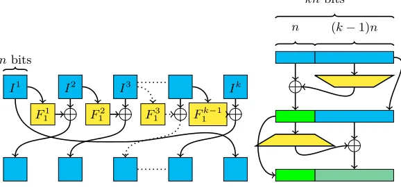
Fig. 1.Round one for Feistel schemes type-1 and type-2
I1 I2 I3
Ik nbits
F1
I1 I2 I3 I4
Ik nbits
F1
1 F12 F
k/2 1
Fig. 2.Round one for type-3 Feistel Scheme and first two rounds of Alternating Feistel Scheme
I1 I2 I3 Ik
nbits
F11 F12 F13 Fk −1 1
knbits
n (k−1)n
The input is always denoted by [I1, I2, . . . , Ik] and the output by [S1, S2, . . . ,
how differences on pairs of input variables will propagate following a differential path, and give relations between pairs of input/output variables. ddenotes the number of rounds. We now define our schemes.
1. Type-1 Feistel Schemes (Fig. 1)
After one round, the output is given by [I2⊕F
1(I1), I3, I4, . . . , Ik, I1] where
F1 is a function fromnbits to nbits. 2. Type-2 Feistel Schemes (Fig. 1)
Here kis even and we set k = 2`. After one round, the output is given by [I2⊕F1
1(I1), I3, I4⊕F12(I3), . . . , I2`⊕F1`(I2`−1), I1] where eachF1s, 1≤s≤` is a function fromnbits tonbits.
3. Type-3 Feistel Schemes (Fig. 2)
After one round, the output is given by [I2 ⊕F11(I1), I3 ⊕F12(I2), I4⊕
F3
1(I3), . . . , Ik⊕F k−1 1 (I
k−1), I1] where eachFs
1, 1≤s≤k−1 is a function fromnbits tonbits.
4. Alternating Feistel Schemes (Fig. 2)
On the input [I1, I2, . . . , Ik], for the first round, we apply a contracting round, i.e. we use a functionF1from (k−1)nbits to nbits and the output is given by [I1⊕F
1([I2, . . . , Ik]), I2, . . . , Ik]. Then for the second round, we apply an expanding round, i.e. we use a function G2 = (G12, G22, . . . , Gk2) where each Gs
2 is a function from n bits to n bits. We set X1 = I1⊕
F1([I2, . . . , Ik]) and then the output after the second round is given by [X1, I2⊕G12(X1), . . . , Ik ⊕Gk2(X1)]. X1 is called an internal variable. Af-ter 2 rounds, we have new inAf-ternal variables. Then we alAf-ternate contracting rounds and expanding rounds. We can also start with an expanding round. In this paper, we will always begin with a contracting round.
We now explain the differential notation. We use plaintext/ciphertexts pairs. In KPA, on the input variables, suppose we set [0,0, ∆30, ∆40, . . . , ∆k0], this means that the pair of messages (i, j) satisfiesI1(i) =I1(j),I2(i) =I2(j), andIs(i)⊕
Is(j) =∆s0, 3≤s≤k. In CPA-1, the same notation means that we chooseI1 and I2 to be constant. We want that the relations between the input variables propagate. Thus we will impose conditions on the internal variables for some round. When we impose conditions on the internal variables in order to get a differential path, we use the notation 0 to mean that the corresponding internal variables are equal in messagesiandj.
3
Overview of the attacks
to the structure of the Feistel scheme. Our attacks consist in using m plain-text/ciphertexts pairs and in counting the number N of couples of these pairs that satisfy the relations between the input and output variables. We then compare Nscheme, the number of such couples we obtain with a generalized scheme, withNperm, the corresponding number for a random permutation. The attack is successful, i.e. we are able to distinguish a permutation generated by a generalized Feistel scheme from a random permutation if the difference
|E(Nscheme)−E(Nperm)| is larger than both standard deviations σNperm and
σNscheme, whereE denotes the expectancy function. In order to compute these values, we need to take into account the fact that the structures obtained from the m plaintext/ciphertext tuples are not independent. However their mutual dependence is very small. To compute σNperm and σNscheme, we will use this well-known formula (see [5], p.97), that we will call the “Covariance Formula”: if x1, . . . xn are random variables, then if V represents the variance, we have
V(Pn
i=1xi) = P n
i=1V(xi) + 2P n−1 i=1
Pn
j=i+1
E(xi, xj)−E(xi)E(xj)
. These kind of computations are also performed in [17].
4
Best attacks on the schemes
For each scheme, we give examples of attacks and describe more precisely KPA and CPA-1 that allow to attack the maximum number of rounds. We always suppose thatk≥3.
4.1 Type-1 Feistel Schemes
For 1 tok−1 rounds, one message is enough, since aftertrounds, 1≤t≤k−1, we haveSk−t+1=I1. This condition is satisfied with probability 1 with a type-1 Feistel scheme and with probability21n when we deal with a random permutation. Thus with one message we can distinguish a type-1 Feistel scheme from a random permutation in KPA and CPA-1.
In Table 1 (left part), we give the general pattern of KPA. The conditions afterpk−2 rounds (p≥3) are given by (2)
S2(i) =S2(j)
I1(i)⊕I1(j) =S3(i)⊕S3(j). We count the number of indices (i, j) such that these conditions are satisfied. Let Nperm (resp. Nscheme) be the number obtained with a random permutation (resp. with a scheme). With a random permutation, these conditions appear at random and we compute the mean value we obtainE(Nperm)' m
2
22n andE(Nscheme)' m
2
22n+ m2
2(p−1)n. The standard deviations satisfy σ(Nperm)'
p
E(Nperm) andσ(Nscheme)'
p
E(Nscheme)'
p
E(Nperm) whenp≥4. This means that we can distinguish between a random permutation and an Type-1 Feistel scheme as soon as 2(pm−21)n ≥
m
Table 1.KPA and CPA-1 on type-1 Feistel Schemes
round ∆10 ∆20∆30...∆k −1 0 ∆
k 0
1 ... ∆10
2 ... ∆10
. . .
k−1 0 ∆10 ...
k ∆10 ... 0
k+ 1 ... ∆10
. . .
pk−2 0 ∆10...
pk−1 0 ∆1 0 ...
pk ∆10 ... 0
. . .
(p+ 1)k−2 0 ∆10...
round 0 ∆20 ∆30 ...∆k −1 0 ∆
k 0 1 ∆20∆30 ... 0
2 ... 0 ∆20
. . .
k−1 0 ∆20 ...
k 0 ∆2
0 ...
k+ 1 ∆20 ... 0
k+ 2 ... 0 ∆2
0 .
. .
pk−1 0 ∆2
0 ...
pk 0 ∆20 ... .
. .
(p+ 1)k−1 0 ∆20 ...
In CPA-1, we know that for 1 to k−1 rounds, one message is enough. For k to 2k−1 rounds, we have a CPA-1 with 2 messages such that ∀s,1 ≤
s ≤ k−1, Is(1) = Is(2). Then with a type-1 Feistel scheme, we obtain with probability 1 that at roundt,S2k−t(1)⊕S2k−t(2) =Ik(1)⊕Ik(2). With a random permutation, the probability to obtain this equality is 21n. For each round, we have to consider different conditions on the input variables. We give now CPA-1 on pk −1 rounds. As shown in Table 1 (right part), we choose the messages such thatI1 takes only one value for all messages. The conditions afterpk−1 rounds are given by (3)
S2(i) =S2(j)
I2(i)⊕I2(j) =S3(i)⊕S3(j). We count the number of indices (i, j) such that these conditions are satisfied. In the appendices, we show that for this CPA-1, we have for a random permutationE(Nperm)' m
2
22n and for a scheme E(Nscheme)' m
2
22n+ m2
2(p−1)n. Using the computation of the variances (see the appendices), we can distinguish between a random permutation and a scheme as long as 2(pm−21)n ≥
m
2n. This gives the conditionm≥2
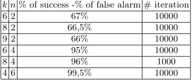
(p−2)n. Since the maximum number of messages is 2(k−1)n, these attacks work forp−2≤k−1 and then withp=k+ 1, we can attack up to (k+ 1)k−1 =k2+k−1 rounds. Table 3 summarizes the complexities for type-1 Feistel schemes. We also give the results of our simulations in Table 2.
4.2 Type-2 Feistel Schemes
Table 4 represents KPA.
We begin with a KPA on 2k+ 2 = 2(k+ 1) rounds where the conditions are: (4)
I1(i) =I1(j)
Table 2.Experimental results for CPA-1 against type-1 Feistel Scheme withk2+k−1 rounds
k n% of success -% of false alarm # iteration
6 2 67% 10000
8 2 66,5% 10000
9 2 66% 10000
6 4 95% 10000
8 4 96% 1000
4 6 99,5% 10000
Table 3.Complexities of the attacks on type-1 Feistel Schemes
d KPA
1→k−1 1
k→2k−1 2n/2 2k→3k−2 2n
. . .
pk−2 2(p−2)n
pk−1 2(p−3/2)n
pk
. .
. 2(p−1)n (p+ 1)k−2
. . .
k2+ 2k−2 2kn
d CPA-1 d CPA-1
1 . .
. 1 ...
k−1
k pk−(p−2) .
.
. 2 ... 2(p−2)n 2k−2 (p+ 1)k−p
2k−1 . .
. 2n/2 ... 3k−2
3k−1 k2+k
. .
. 2n ... 2(k−1)n 4k−3 k2+k−1
For a scheme, we obtain 2m2n2 + m2
2(k+1)n. As previously, the computation of the standard deviations shows that we can distinguish between a random permuta-tion and a scheme as long as m2
2(k+1)n ≥ m
2n. This gives the condition m≥ 2 kn, which is the maximum number of messages. More generally, after 2p rounds,
p≥3, we use the same attack with the conditions: (5)
I1(i) =I1(j)
I2(i)⊕I2(j) =Ss(i)⊕Ss(j). where t is defined by s = k−2(p−1) if 1≤p≤`
s=k−2(u−1) ifp=k+ 2u, 1≤u≤` s= 2k−2(u−1) ifp= 2k+ 2u, 1≤u≤2
We count the number of indices (i, j) such that these conditions are satisfied. For a random permutation this is about 2m22n. For a scheme, we obtain
m2 22n+
m2 2pn. Again we can distinguish between a random permutation and a scheme as long as 2mpn2 ≥
m
2n and we obtain that the number of messages is 2(p−1)n. Thus for
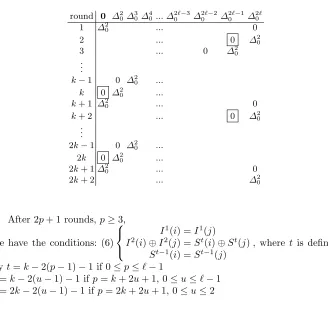
Table 4.KPA on type-2 Feistel Schemes
round 0 ∆20 ∆30 ∆40 ...∆20`−3∆ 2`−2 0 ∆
2`−1 0 ∆
2` 0
1 ∆20 ... 0
2 ... 0 ∆20
3 ... 0 ∆2
0 .
. .
k−1 0 ∆20 ...
k 0 ∆20 ...
k+ 1 ∆2
0 ... 0
k+ 2 ... 0 ∆20
. . .
2k−1 0 ∆20 ... 2k 0 ∆2
0 ...
2k+ 1∆20 ... 0
2k+ 2 ... ∆20
After 2p+ 1 rounds,p≥3, we have the conditions: (6)
I1(i) =I1(j)
I2(i)⊕I2(j) =St(i)⊕St(j)
St−1(i) =St−1(j)
, where t is defined byt=k−2(p−1)−1 if 0≤p≤`−1
t=k−2(u−1)−1 ifp=k+ 2u+ 1, 0≤u≤`−1
t= 2k−2(u−1)−1 ifp= 2k+ 2u+ 1, 0≤u≤2
We count the number of indices (i, j) such that this condition is satisfied. For a random permutation this is about m2
23n. For a scheme, we obtain m2 23n+
m2 2(p+1)n. The variance is about the square root of the mean value. Thus we can distinguish between a random permutation and a scheme as long as 2(pm+1)2n ≥
m
23n/2 and we
obtain that the number of messages is 2(p−1/2)n.
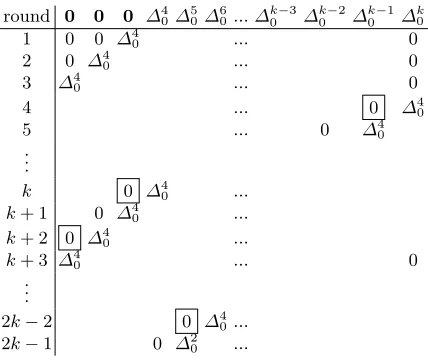
For CPA-1, we can impose conditions on a given number of input variables. We give in Table 5 an example of an attack for which we consider messages whereI1,I2, I3 are given constant values. Then we will generalize.
The conditions after 2k−1 rounds are given by (7)
S4(i) =S4(j)
I4(i)⊕I4(j) =S5(i)⊕S5(j). We count the number of indices (i, j) such that these conditions are satisfied. For a random permutation this is about 2m22n. For a scheme, we obtain2m2n2+
m2
2(k−2)n. Since again the variance is about the square root of the mean value, we can distinguish between a random permutation and a scheme as long as 2(km−22)n ≥
m
2n. This gives the conditionm≥2
Table 5.CPA-1 on type-2 Feistel Schemes
round 0 0 0 ∆40 ∆05 ∆60...∆k0−3 ∆ k−2 0 ∆
k−1 0 ∆
k 0
1 0 0 ∆40 ... 0
2 0 ∆4
0 ... 0
3 ∆40 ... 0
4 ... 0 ∆40
5 ... 0 ∆40
. . .
k 0 ∆40 ...
k+ 1 0 ∆40 ...
k+ 2 0 ∆4
0 ...
k+ 3 ∆40 ... 0
. . .
2k−2 0 ∆40... 2k−1 0 ∆20 ...
(i, j) such that (8)S6(i) =S6(j) . For a random permutation this is about m2 2n. For a scheme, we obtain m2
22n+ m2
2(k−3)n. The variance is about the square root of the mean value. Thus we can distinguish between a random permutation and a scheme as long as2(km−23)n ≥
m
2n/2. This gives the conditionm≥2
(k−3−1/2)n. Since the maximum number of messages is 2(k−3)n, we get a CPA-1 for 2k−2 rounds. More generally, if we suppose that for the input variables, we have I1, . . . , Ip are constant (p≤k−1), we can perform the same kind of attacks. It is easy to check that we can attack up to 2k−p+ 2 rounds and we need exactly 2(k−p)n. In order to get the best CPA-1 for each round, we will change the conditions on the input variables. For example, for k+ 1,k+ 2 andk+ 3 rounds, we choose
I1, . . . Ik−1 to be constant, then we will haveI1, . . . Ik−2 constant, and so on. Table 6 summarizes the complexities for type-2 Feistel schemes.
4.3 Type-3 Feistel Schemes
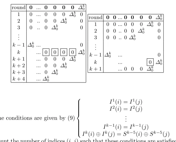
We will present our attacks when k = 2` is even and give only the results for k odd. We begin with KPA. For one round, we need one message, we just have to check if I1 = S2`. With a random permutation, this happens with probability 21n and with a scheme with probability one. Suppose we want to attack drounds with 2 ≤ d≤k. We wait until we have 2 messages such that
I1(1) = I1(2), . . . , Id−1(1) = Id−1(2). Then we test if Id−1(1)⊕Id−1(2) =
Sk(1)⊕Sk(2). With a random permutation, this happens with probability 21n and with a scheme with probability one. Moreover, from the birthday paradox, if we have 2(d−21)n messages, we get 2 messages with the given conditions with a
Table 6.Complexities of the a attacks on type-2 Feistel Schemes
d KPA
1 1
2 2n/2 3 2n/2
. . .
2p 2(p−1)n 2p+ 1 2(p−1/2)n
. . .
2k 2(k−1)n 2k+ 1 2(k−1/2)n 2k+ 2 2kn
d CPA-1
1 1
2 . .
. 2
k
k+ 1 2n/2
k+ 2 2n/2 .
. .
k+v 2(v−2)n .
. .
2k+ 1 2(k−1)n
Table 7.KPA and CPA-1 on type-3 Feistel Schemes
round 0 ... 0 0 0 0 ∆k0 1 0 ... 0 0 0 ∆k
0 0 2 0 .. 0 0 ∆k0 0
3 0 .. 0 ∆k0 0
. . .
k−1 ∆k
0 ... 0
k ... 0 0 0 0 ∆k0
k+ 1 ... 0 0 0 ∆k0
k+ 2 ... 0 0 ∆k0
k+ 3 ... 0 ∆k0
k+ 4 ...∆k 0
round 0 0...0 0 0 0 ∆k0 1 0 0 ... 0 0 0 ∆k0 0 2 0 0 .. 0 0 ∆k
0 0 3 0 0 .. 0∆k
0 0
. . .
k−1 ∆k
0 ... 0
k ... 0 ∆k
0
k+ 1 ... 0 0 0 ∆k 0
The conditions are given by (9)
I1(i) =I1(j)
I2(i) =I2(j) .. .
Ik−1(i) =Ik−1(j)
Ik(i)⊕Ik(j) =Sk−5(i)⊕Sk−5(j) We count the number of indices (i, j) such that these conditions are satisfied. For a random permutation this is about 2mkn2. For a scheme, we obtain
m2
2kn + m2
2(k+3)n. We can distinguish between a random permutation and a scheme as long as
m2 2(k+3)n ≥
m
2ln. This gives m≥2
(l+3)n. We can perform the same kind of attack for k+t rounds, with t ≤ `+ 1. We can attack up to k+`+ 1 rounds. For
k+`+ 1, we need the maximum number of messages i.e. 2kn.
For CPA-1, it is easy to see that after one round, one message is sufficient. We just have to check ifSk =I1. For 2 rounds, we choose 2 messages such thatI1(1) =
we can distinguish between the two permutations with only 2 messages. More generally, fordrounds withd≤k, we choose 2 messages such thatIs(1) =Is(2) for 1≤s≤k−1 and then we check if Sk(1)⊕Sk(2) =Id(1)⊕Id(2). With a random permutation this happens with probability 21n, but with a scheme, the probability is one. Thus we can distinguish between the two permutations with only 2 messages. We can attack up to krounds. For k+ 1 rounds, we have the following CPA-1 described in Table 7 (right part). We choosem messages such that I1, I2, . . . , Ik−1 have a constant value. We count the number of (i, j) such thatIk(i)⊕Ik(j) =Sk−1(i)⊕Sk−1(j). For a random permutation this is about
m2
2n. For a scheme, we obtain m2
2n + m2
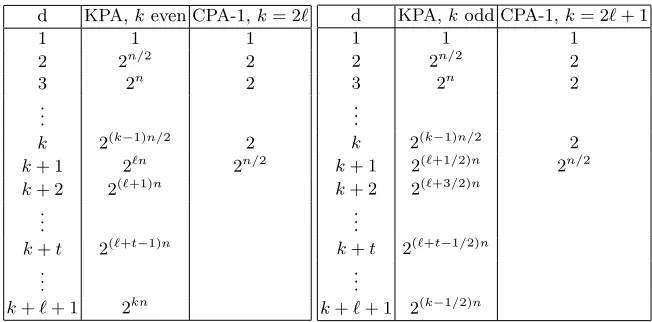
2n. We can distinguish between a random permutation and a scheme when the number of messagesmis about 2n/2. Table 8 gives KPA complexities ford≤k+`+ 1 and CPA-1 ones ford≤k+ 1.
Table 8.Attacks on type-3 Feistel Schemes
d KPA,keven CPA-1,k= 2`
1 1 1
2 2n/2 2
3 2n 2
. . .
k 2(k−1)n/2 2
k+ 1 2`n 2n/2
k+ 2 2(`+1)n .
. .
k+t 2(`+t−1)n .
. .
k+`+ 1 2kn
d KPA,kodd CPA-1,k= 2`+ 1
1 1 1
2 2n/2 2
3 2n 2
. . .
k 2(k−1)n/2 2
k+ 1 2(`+1/2)n 2n/2
k+ 2 2(`+3/2)n .
. .
k+t 2(`+t−1/2)n .
. .
k+`+ 1 2(k−1/2)n
4.4 Alternating Feistel Schemes
Here we will describe our best attacks on alternating Feistel schemes. After one round, we have [I2, I3, . . . , Ik] = [S2, S3, . . . , Sk]. Thus we choose one message and we check if this condition is satisfied. With a random permutation, this happens with probability 2(k−11)n and with a scheme the probability is one. Thus with one message we can distinguish a random permutation from a permutation obtained with an alternating scheme. After 2 rounds, in CPA-1, we choose 2 messages such that∀s,2≤s≤k, Is(1) =Is(2) and then we check if I1(1)⊕
are better KPA, as we can see now. We have the following CPA-1, described in table 9 (right part), where ∆denotes [∆2
0, ∆30, ∆40, . . . , ∆k0].
At each odd round, the probability to have the first zero is 1/2n. So we have the probability of 1/2np to have the equalities on the output:S2(1)⊕S2(2) =
I2(1)⊕I2(2) and S1(1) = S1(2) when we follow the path. But we can also have this equalities without the path. For a random permutation, the proba-bility to have this is equal to 21n ×
1 2(k−1)n =
1
2kn. So the number of such pair of points will be greater for an alternating scheme when p ≤ k, i.e. d = 2p. The number of messages is m = 2np/2 = 2nd/4. This is a CPA-1 complexity of course, but we can transform slightly the attack in order to have the same complexity in KPA and CPA-1, as shown in Table 9 (left part). For example,
Table 9.KPA and CPA-1 on Alternating Feistel Schemes
round ∆1 ∆
1 0 ∆
2 0 ∆
3 0 ∆
4 0 ∆
. . . ... 2p−1 0 ∆
2p 0 ∆
round 0 ∆
1 0 ∆
2 0 ∆
3 0 ∆
4 0 ∆
. . . ... 2p−1 0 ∆
2p 0 ∆
we obtain here, after 2 rounds a KPA with 2n2 messages (notice that the CPA-1
complexity of the previous attack was better). These attacks are valid until we reach 2krounds. We explain now how to attack more rounds if we use the co-variance formula as mentioned in Section 3. We keep the same kind of attacks. After 2prounds with p≥ k, in KPA, we count the number of (i, j) such that (1)
S1(i) =S1(j)
∀s,2≤s≤k, Is(i)⊕Is(j) =Ss(i)⊕Ss(j)
Let Nperm (resp. Nscheme) be the number obtained with a random permuta-tion (resp. with a scheme). With a random permutapermuta-tion, these condipermuta-tions ap-pear at random. ThusE(Nperm)' m
2
2kn. For a scheme, we obtainE(Nscheme) = m(m−1)
2 1 2kn+
1 2pn+
1 2(k+p−1)n
' m2 2kn+
m2
2pn. As usual, the standard deviations sat-isfy σ(Nperm)'
p
E(Nperm) and σ(Nscheme)'
p
E(Nscheme)'
p
E(Nperm). This means that we can distinguish between a random permutation and an alter-nating scheme as soon as m2
2pn ≥ m
2kn/2, i.e.m≥2
(p−k
2)n. Thus we obtain a KPA
with about 2(p−k
2)n messages. Since the number of messages cannot exceed 2kn,
rounds. If we want to attack an odd round, for example round 2p−1, the last condition on the internal variable is imposed at round 2p−3 and then we will count the number of (i, j) such that∀s,2≤s≤k, Is(i)⊕Is(j) =Ss(i)⊕Ss(j). By computing the mean values and the standard deviations, we obtain that
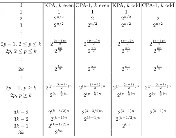
m'2(p−(k−21))n. We now summarize all the complexities in Table 10.
Table 10.Complexities of the attacks on Alternating Feistel Schemes
d KPA,keven CPA-1,keven KPA,kodd CPA-1,kodd
1 1 1 1
2 2n/2 2 2n/2 2
3 2n/2 2n/2 2n/2 2n/2
. . .
2p−1, 2≤p≤k 2(p−21)n 2 (p−1)n
2 2
(p−1)n
2 2
(p−1)n
2
2p, 2≤p≤k 2pn2 2
pn
2 2
pn
2 2
pn
2
. . .
2k 2kn2 2
kn
2 2
kn
2 2
kn
2
. . .
2p−1,p≥k 2(p−(k−21))n 2(p− (k−1)
2 )n 2(p− (k−1)
2 )n 2(p− (k−1)
2 )n
2p,p≥k 2(p−k
2)n 2(p−k2)n 2(p−k2)n 2(p−k2)n
. . .
3k−3 2(k−3/2)n 2(k−3/2)n 2(k−1)n 2(k−1)n 3k−2 2(k−1)n 2(k−1)n 2(k−1/2)n
3k−1 2(k−1/2)n 2kn
3k 2kn
5
Conclusion
References
1. William Aiello and Ramarathnam Venkatesan. Foiling Birthday Attacks in Length-Doubling Transformations - Benes: A Non-Reversible Alternative to Feistel. In Ueli M. Maurer, editor,Advances in Cryptology – EUROCRYPT ’96, volume 1070 ofLecture Notes in Computer Science, pages 307–320. Springer-Verlag, 1996. 2. Ross J. Anderson and Eli Biham. Two Practical and Provably Secure Block
Ci-phers: BEAR and LION. In Dieter Gollman, editor,Fast Software Encryption, vol-ume 1039 ofLecture Notes in Computer Science, pages 113–120. Springer-Verlag, 1996.
3. Andrey Bogdanov and Vincent Rijmen. Zero-Correlation Linear Cryptanalysis on Block Cipher. Cryptology ePrint archive: 2011/123: Listing for 2011.
4. Charles Bouillaguet, Orr Dunkelamn, Gaetan Laurent, and Pierre-Alain Fouque. Attacks on hash Functions based on Generalized Feistel schemes. Application to Reduced-RoundLesamntaandSHAvite−3512. In Alex Biryukov, Guang Gong, and Douglas R. Stinson, editors,Selected Areas in Cryptographyl – SAC ’10, volume 6544 ofLecture Notes in Computer Science, pages 18–35. Springer-Verlag, 2010. 5. Paul G.Hoel, Sidney C.Port, and Charles J.Stone. Introduction to Probability
The-ory. Houghton Mifflin Company, 1971.
6. Viet Tung Hoang and Phillip Rogaway. On Generalized Feistel Networks. In Tel Rabin, editor,Advances in Cryptology – CRYPTO 2010, volume 6223 ofLecture Notes in Computer Science, pages 613–630. Springer-Verlag, 2110.
7. Subariah Ibrahim and f Mohd Aizaini Mararof. Diffusion Analysis of Scalable Feistel Networks. World Academy of Science, Engineering and Technology, 5:98– 101, 2005.
8. Charanjit S. Jutla. Generalized Birthday Attacks on Unbalanced Feistel Networks. In Hugo Krawczyk, editor,Advances in Cryptology – CRYPTO ’98, volume 1462 ofLecture Notes in Computer Science, pages 186–199. Springer-Verlag, 1998. 9. Lars R. Knudsen. DEAL - A 128-bit Block Cipher. Technical Report 151,
Univer-sity of Bergen, Department of Informatics, Norway, february 1998.
10. Lars R. Knudsen and Vincent Rijmen. On the Decorrelated Fast Cipher (DFC) and Its Theory. In Lars R. Knudsen, editor, Fast Software Encrytion – FSE ’99, volume 1636 ofLecture Notes in Computer Science, pages 81–94. Springer-Verlag, 1999.
11. Michael Luby and Charles Rackoff. How to Construct Pseudorandom Permutations from Pseudorandom Functions. SIAM J. Comput., 17(2):373–386, 1988.
12. Moni Naor and Omer Reingold. On the Construction of Pseudorandom Permuta-tions: Luby-Rackoff Revisited. J. Cryptology, 12(1):29–66, 1999.
13. Jacques Partarin. Security of balanced and unbalanced Feistel schemes with linear non equalities. Cryptology ePrint archive: 2010/293: Listing for 2010.
14. Jacques Patarin. New Results on Pseudorandom Permutation Generators Based on the DES Scheme. In Joan Feigenbaum, editor, Advances in Cryptology – CRYPTO ’91, volume 576 ofLecture Notes in Computer Science, pages 301–312. Springer-Verlag, 1991.
15. Jacques Patarin. Generic Attacks on Feistel Schemes. In Colin Boyd, editor, Advances in Cryptology – ASIACRYPT 2001, volume 2248 of Lecture Notes in Computer Science, pages 222–238. Springer-Verlag, 2001.
17. Jacques Patarin, Val´erie Nachef, and Cˆome Berbain. Generic Attacks on Unbal-anced Feistel Schemes with Contracting Functions. In Xuejia Lai and Kefei Chen, editors,Advances in Cryptology – ASIACRYPT 2006, volume 4284 ofLecture Notes in Computer Science, pages 396–411. Springer-Verlag, 2006.
18. Jacques Patarin, Val´erie Nachef, and Cˆome Berbain. Generic Attacks on Unbal-anced Feistel Schemes with Expanding Functions. In Kaoru Kurosawa, editor, Advances in Cryptology – ASIACRYPT 2007, volume 4833 of Lecture Notes in Computer Science, pages 325–341. Springer-Verlag, 2007.
19. Bruce Schneier and John Kelsey. Unbalanced Feistel Networks and Block Cipher Design. In Dieter Gollmann, editor,Fast Software Encrytion – FSE ’96, volume 1039 ofLecture Notes in Computer Science, pages 121–144. Springer-Verlag, 1996. 20. Joana Treger and Jacques Patarin. Generic Attacks on Feistel Networks with Internal Permutations. In Bart Preneel, editor, Progresses in Cryptology – AFRICACRYPT ’09, volume 5580 of Lecture Notes in Computer Science, pages 41–59. Springer-Verlag, 2009.
21. Emmanuel Volte, Val´erie Nachef, and Jacques Patarin. Improved Generic Attacks on Unbalanced Feistel Schemes with Expanding Functions. In Kaoru Kurosawa, editor,Advances in Cryptology – ASIACRYPT 2010, volume 6477 ofLecture Notes in Computer Science, pages 94–111. Springer-Verlag, 2007.
22. Aaram Yun, Je Hong Park, and Jooyoung Lee. Lai-Massey Scheme and Quasi-Feistel Networks. Cryptology ePrint archive: 2007/347: Listing for 2007.
23. Y. Zhen, T. Matsumoto, and H. Imai. On the Construction of Block Ciphers provably secure and not relying on any unproved Hypotheses. In Gilles Brassard, editor, Advances in Cryptology – CRYPTO ’89, volume 435 of Lecture Notes in Computer Science, pages 461–480. Springer-Verlag, 1990.
A
An example of Computation of the Mean Value and
the Variance for Random Permutations
Very often in cryptographic attacks based on the computations of variance V
and mean valueE we have V 'E, particularly when we deal with differential attacks. We will prove this precisely here for the CPA-1 given in section 4.1. Similar proofs have also been done for other cases.
First we compute the mean value denoted by E(Nperm). We have ∀i, 1 ≤
i≤m, I1(i) = 0. Herem'2(p−2)n. The inputs are pairwise distinct. Letδij = 1 if (∗) is satisfied δij = 0 otherwise. Then Nperm = Pi<jδij, E(Nperm) =
P
i<jE(δij).E(δij) =P rf∈RBkn[S2(i) =S2(j) andI2(i)⊕I2(j) =S3(i)⊕S3(j)] Case 1:I2(i) =I2(j). Here E(δij) =P rf∈RBkn[S2(i) =S2(j) andS3(i) =S3(j)] = 2(k2−kn2)−n1−1 =
1 22n×
1− 1 2(k−2)n
1− 1 2kn
Case 2:I2(i)6=I2(j). ThenE(δij) =P rf∈RBkn[S2(i) =S2(j) andI2(i)⊕I2(j) =
S3(i)⊕S3(j)] =2
(k−2)n 2kn−1 =
1 22n ×
1 1− 1
2kn .
Let α be the number of (i, j) such that I2(i) = I2(j). Then E(Nperm) =
α2(k2−kn2)−n1−1
+m(m2−1)−α22(knk−−2)1n
= [m(m2·22−n1)− α 2kn]×
1 1− 1
2kn . We can assume thatα= m(m2·2−n1)+ 0(
m
√
E(Nperm) = [ m(m−1)
2·22n − 1 2kn
m(m
−1) 2·2n +0(
m
√
2n)
]× 1 1− 1
2kn
= m(m2·22−n1)× 1− 1
2(k−1)n
1− 1 2kn
+
O( m 2k+ 12
). Finally, this gives m(m−1)
2·22n
1− 1 2(k−1)n+
1 2kn
+O( m 2(k+ 12)n
)≤E(Nperm)≤
m(m−1) 2·22n +O(
m 2(k+ 12)n
). We now gives the main steps in order to compute the standard deviation. We will use the “covariance formula ” given in Section 3 in order to computeV(Nperm). We have:V(δij) =E(δ2ij)−E(δij)2=E(δij)−E(δij)2.
Case 1:I2(i) =I2(j).V(δij) = 212n× 1− 1
2(k−2)n
1− 1 2kn
− 1 22n×
1− 1 2(k−2)n
1− 1 2kn
)2. This gives:
V(δij) = 212n
1− 1 22n −
1 2(k−2)n +
3 2kn −
2 2(k+2)n −
2 2(2k−2)n +
5 22kn −
3 2(2k+2)n − 3
2(3k−2)n
i
+O( 1 23kn)
Case 2: I2(i)6=I2(j).V(δij) =212n × 1 1− 1
2kn
− 1 22n ×
1 1− 1
2kn
2
. We obtain
V(δij) = 212n
1− 1 22n+
1 2kn −
2 2(k+2)n +
1 22kn −
3 2(2k+2)n
i
+O(231kn).
Since we want to use the covariance formula, we have to evaluate E(δij)E(δqr) andE(δijδqr). We explain the case wherei, j, q, rare pairwise distinct. The case where in{i, j, q, r}we have exactly 3 values is similar. The total number of out-puts is given byA= 2kn(2kn−1)(2kn−2)(2kn−3) = 24kn(1− 6
2kn+ 11 22kn−
6 23kn). Then A1 = 241kn
1 + 2kn6 + 25 22kn +O(
1 23kn)
. We first evaluate E(δij)E(δqr). We have to study several cases:
1. I2(i)6=I2(j) andI2(q)6=I2(r). Then
E(δij)E(δqr) = 214n
1 1− 1
2kn
2
= 1 24n(1 +
2 2kn +
3 22kn +O(
1 23kn)).
2. (I2(i) =I2(j) andI2(q)6=I2(r)) or (I2(i)6=I2(j) andI2(q) =I2(r)). Then
E(δij)E(δqr) = 214n
1− 1 2(k−2)n (1− 1
2kn)2
.
E(δij)E(δqr) = 214n(1− 1 2(k−2)n+
2 2kn −
2 2(2k−2)n+
3 22kn −
3
2(3k−2)n+O( 1 23kn)). 3. I2(i) =I2(j) andI2(q) =I2(r). ThenE(δij)E(δqr) = 214n×
(1− 1 2(k−2)n)
2
(1− 1 2kn)
2
= 241n(1− 2 2(k−2)n +
2 2kn +
1 2(2k−4)n −
4 2(2k−2)n +
3 22kn +
2 2(3k−4)n −
6 2(3k−2)n +
O( 1 23kn)).
We compute E(δijδqr). Again we have to consider several cases. We give the main case:I2(i)6=I2(j),I2(q)6=I2(r) andI2(i)⊕I2(j)⊕I2(q)⊕I2(r)6= 0. In that case, S3(j) = I2(i)⊕I2(j)⊕S3(i) 6=S3(i). There are 2kn possibilities forS(i). WhenS(i) is fixed, there are 2(k−2)n possibilities for S(j), sinceS2(j) andS3(j) are fixed. Now forS(q) there are 6 possibilities:
1- S2(q) 6= S2(i) (we have S2(i) = S2(j)). Then S2(r) = S2(q) 6=S2(i). Since
S3(r) = S3(q)⊕I2(q)⊕I2(r), we have S3(q) 6= S3(r). Thus there are (2n− 1)2(k−1)n possibilities forS(q) and 2(k−2)npossibilities forS(r) This gives (2n− 1)22k−3)n possibilities for (S(q), S(r)).
2- S2(q) =S2(i) =S2(j) andS3(q) =S3(i)⊕I2(q)⊕I2(r).
possibilities for (S(q), S(r)).
3- S2(q) =S2(i) =S2(j) andS3(q) =S3(j)⊕I2(q)⊕I2(r).
There are 2(k−2)npossibilities forS(p) and 2(k−2)n−1 possibilities forS(r). This gives 22(k−2)n(22(k−2)n−1) possibilities for (S(q), S(r))
4- S2(q) = S2(i) = S2(j) and S3(q) = S3(i). This gives (22(k−2)n−1)22(k−2)n possibilities for (S(q), S(r))
5- S2(q) = S2(i) = S2(j) and S3(q) = S3(j). This gives again (22(k−2)n − 1)22(k−2)n possibilities for (S(q), S(r))
6-S2(q) =S2(i) =S2(j) and we are not in cases b,c,d, e. This gives (22(k−2)n− 4)22(k−2)n possibilities for (S(q), S(r))
Finally, the number of possible outputs for S(i), S(j), S(q), S(r) in this case 1 is given by B = 2(4k−4)n1− 4
2kn
andE(δijδqr) = BA = 241n
1 +2kn2 + 1 22kn +
O( 1 23kn)
. Thus E(δij)E(δqr)−E(δijδqr) = 214n
− 2 22kn +O(
1 23kn)
. The term
−2m4
4·24n·22kn m2
22n sincem2kn The other cases areI2(i) = (j), I2(q)6=I2(r),
I2(i)6=I2(j),I2(q)6=I2(r) andI2(i)⊕I2(j)⊕I2(q)⊕I2(r) = 0 andI2(i) =I2(j) andI2(q) =I2(r). The study is similar to the main case.
All the computations show thatV(Nperm) = m(m2·22−n1)(1− 1 22n+O(
1 2kn)). ThusV(Nperm)'E(Nperm) as claimed.
B
Computation of the Mean Value and the Variance for
Feistel Type-1 Schemes
Here we suppose that p= 4. For anypthe computations are similar. We intro-duce the internal variables:
X1=I
2⊕f1(I1), X2=I3⊕f2(X1), X3=I4⊕f3(X2). . .
Xk−1=I
k⊕fk−1(Xk−2), Xk =I1⊕f3(Xk−1), Xk+1=X1⊕fk−1(Xk). . .
X2k−1=Xk−1⊕f2k−1(X2k−2), X2k =Xk⊕f2k(X2k−1). . .
X3k−1=X2k−1⊕f3k−1(X3k−2), X3k =X2k⊕f3k(X3k−1). . .
X4k−1=X3k−1⊕f4k−1(X4k−2)
For ` ≥ k−1, X` depends on all the input variables. Thus we can assume, since the internal functions are randomly chosen, that for ` ≥ k−1,the in-ternal variables X` are completely independent. After 4k−1 rounds the out-put is given by: [S1, S2, S3, . . . , Sk] = [X4k−1, X3k, X3k+1, . . . , X4k−2]. where
S3 =I2⊕f1(I1)⊕fk+1(Xk)⊕f2k+1(X2k)⊕f3k−1(X3k). Thus the following conditions:
(∗) S2(i) =S2(j),andI2(i)⊕I2(j) =S3(i)⊕S3(j) are equivalent to (∗∗)X3k(i) =X3k(j) andfk+1(Xk(i))⊕f2k+1(X2k(i)) =fk+1(Xk(j))
⊕f2k+1(X2k(j))
In order to computeE(δij), we consider 2 cases.
1. X3k(i) =X3k(j) and (Xk(i), X2k(i)) = (Xk(j), X2k(j)). The probability is 1
23n.
2. X3k(i) = X3k(j), (Xk(i), X2k(i)) 6= Xk(j), X2k(j)) and fk+1(Xk(i))⊕
f2k+1(X2k(i)) =fk+1(Xk(j))⊕f2k+1(X2k(j)). The probability is 1 2n(1− 1
22n) 1 2n =
1 22n−
Finally E(δij) = 212n + 1 23n −
1
24n and E(Ntype1) =
m(m−1) 2
1 22n +
1 23n −
1 24n
.
V(δij) =E(δij)−(E(δij))2=221n + 1 23n −
2 24n−
2 25n+
1 26n+
2 27n−
1
28n. We will use the covariance formula:V(Ntype1) =V(Pi<jδij) +P 1<j
q<r
(i,j)6=(q,r)
[E(δijδqr)−
E(δij)E(δqr)].E(δij)E(δqr) = (212n+ 1 23n−
1 24n)
2= 1 24n+
2 25n−
1 26n−
2 27n+
1 28n. We now computeE(δijδqr). We explain the case wherei, j, q, rare pairwise distinct. The case where in {i, j, q, r} we have exactly 3 values is similar. Wheni, j, q, r
are pairwise distinct, the conditions (∗∗) are satisfied for the pairs (i, j) and (q, r). Then we have to study several cases.
1. X3k(i) =X3k(j),X3k(q) =X3k(r), (Xk(i), X2k(i)) = (Xk(j), X2k(j)) and (Xk(q), X2k(q)) = (Xk(r), X2k(r)). The probability is 1
26n.
2. X3k(i) =X3k(j),X3k(q) =X3k(r), (Xk(i), X2k(i)) = (Xk(j), X2k(j)) and (Xk(q), X2k(q)) 6= (Xk(r), X2k(r)) and fk+1(Xk(q))⊕f2k+1(X2k(q)) =
fk+1(Xk(r))⊕f2k+1(X2k(r)). Then the probability is given by 1 2n×
1 2n × 1
22n(1− 1 22n)×
1 2n =
1 25n−
1 27n.
3. X3k(i) = X3k(j), X3k(q) = X3k(r), (Xk(i), X2k(i)) = (6 Xk(j), X2k(j)) and (Xk(q), X2k(q)) = (Xk(r), X2k(r)) andfk+1(Xk(i)⊕f2k+1(X2k(i)) =
fk+1(Xk(j))⊕f2k+1(X2k(j)). As in the previous case, the probability is given by 215n −
1 27n.
4. X3k(i) = X3k(j), X3k(q) = X3k(r), (Xk(i), X2k(i)) = (6 Xk(j), X2k(j)), (Xk(q), X2k(q)) = (Xk(i), X2k(i)), (Xk(r), X2k(r)) = (Xk(j), X2k(j))
fk+1(Xk(i)⊕f2k+1(X2k(i)) =fk+1(Xk(j))⊕f2k+1(X2k(j)). The probabil-ity is given by 21n×
1 2n×
1 22n(1−
1 22n)×
1 22n ×
1 22n×
1 2n =
1 27n−
1 29n. 5. X3k(i) = X3k(j), X3k(q) = X3k(r), (Xk(i), X2k(i)) = (6 Xk(j), X2k(j)),
(Xk(r), X2k(r)) = (Xk(i), X2k(i)), (Xk(q), X2k(q)) = (Xk(j), X2k(j)),
fk+1(Xk(i)⊕f2k+1(X2k(i)) = fk+1(Xk(j))⊕f2k+1(X2k(j)). Again the probability is given by 217n−
1 29n.
6. X3k(i) = X3k(j), X3k(q) = X3k(r), (Xk(i), X2k(i)) = (6 Xk(j), X2k(j)) and (Xk(q), X2k(q)) 6= (Xk(r), X2k(r)), we are not in cases 4 and 5 and
f2k+1(X2k(i)) =fk+1(Xk(j))⊕f2k+1(X2k(j)) andfk+1(Xk(q))
⊕f2k+1(X2k(q)) =fk+1(Xk(r))⊕f2k+1(X2k(r)). Then the probability is 1
2n× 1
2n×[(1− 1
22n)×(1− 1
22n)−(1− 1 22n)×
1 22n×
1 22n]×
1 2n =
1 24n−
2 26n
1 210n. Finally we obtain E(δijδqr) = +225n −
1 26n
4 27n −
2 29n +
1
210n and E(δijδqr)−
E(δij)E(δqr) =267n − 2 29n+
1
210n. Thus in
P
1<j q<r
(i,j)6=(q,r)
[E(δijδqr)−E(δij)E(δqr)] the term 2m7n4
m2
22n sincem'2
2n in our attack.
Our computations show that the CPA-1 onpk−1 rounds with p≤k+ 2, we have: E(Nperm) ' m
2
22n, E(Ntype1) ' m
2
22n + m2
2(p−1)n, V(Nperm) ' m
2
22n and,
σ(Nperm)' 2mn,V(Ntype1)' m
2
22n, andσ(Ntype1)'2mn. Thus we can distinguish a permutation obtained by a Type 1 Feistel scheme from a random permutation as soon as |E(Nperm)−E(Ntype1)| ≥ σ(Nperm), |E(Nperm)−E(Ntype1)| ≥
σ(Ntype1) i.e. as soon as m
2
2(p−1)n ≥ m