ABSTRACT
GOKCE, MAHMUT ALI. Optimization of Sourcing Decisions in Supply Chains. (Under the direction of Dr. Russell E. King, Dr. Jeffery A. Joines, and Dr. Michael G. Kay.)
Sourcing decisions in supply chains traditionally are made solely based on cost considerations. Typically sourcing models or decision-making procedures are either ad hoc or proprietary. In this dissertation a meta-heuristic-based optimization approach is developed and applied to sourcing decisions in several different apparel supply chains.
To solve this kind of a large combinatorial problem, two issues need to be addressed: the solution methodology and the performance measure to be used. We develop a simulation-optimization methodology based on genetic algorithms (GA). Deficiencies of some of the current supply chain performance measures are addressed and a new performance measure, GMROILS, is developed. The GA with complex evaluations is used to determine optimal sourcing decisions for a seasonal item in an apparel supply chain with GMROILS as the performance measure. The Sourcing Simulatorâ is used for the simulation. Results show that the proposed methodology produces very good results.
results and we determine that best GMROILS is achieved generally when number of reorders is maximized.
Next, we develop a constrained GA with complex evaluations. First, the constrained GA is used with the same experimental design using GMROI as the main performance measure with a 95% service level constraint. Results from the experimentation are in agreement with the previous results, i.e. the leanest and most flexible and responsive supply chain yields the best performance. We also conclude that GMROILS is an appropriate performance measure to be used in these cases.
The constrained GA with complex evaluations was applied to a industry-supplied case study. We look at the sourcing of workpants to large, discount retail chain. The problem is to find the best inventory policy for the supplier of the workpants in order to provide a 95% service level to the retailer while maximizing GMROI (the objective defined by the supplier). We use the constrained GA with complex evaluations to find the best combination of presentation stock levels and target week of supply for the 420 SKUs so as to maximize GMROI while keeping 95% service level. We compare results from the optimizer to some classical alternatives including the existing policy.
OPTIMIZATION OF SOURCING DECISIONS IN SUPPLY
CHAINS
by
MAHMUT ALÌ GÖKÇE
A dissertation submitted to the Graduate Faculty of North Carolina State University
In partial fulfillment of the Requirements for the Degree of
Doctor of Philosophy
INDUSTRIAL ENGINEERING
Raleigh
2002
APPROVED BY:
___________________________ ___________________________
Dr. Thom J. Hodgson Dr. Michael G. Kay
Co-Chair of Advisory Committee
___________________________ ___________________________
Dr. Russell E. King Dr. Jeffery A. Joines
BIOGRAPHY
Mahmut Ali Gokce was born in Ìzmir, Turkey on June, 01 1975. After finishing Ìzmir Science High School, he attended Bilkent University in Ankara, Turkey. He received his B.S. in industrial engineering from Bilkent University in 1997. In August 1997, he started his graduate study at North Carolina State University Department of Industrial Engineering. He worked as a teaching assistant and research assistant in the industrial engineering department. He received his M.S. degree in the industrial engineering under the direction of Dr. Russell E. King. In Fall 1999, he enrolled in the Ph.D. program in the industrial engineering department of North Carolina State University. He worked as a research assistant for National Textile Center from 1999 to 2001. He was employed as a research assistant in the industrial engineering department in 2002.
ACKNOWLEDGEMENTS
I would like to extend my deepest and most sincere thanks to Dr. Russell E. King for his continuos support, patience, advice, trust, and encouragement through the years. I also would like to thank Dr. Jeffery A. Joines, Michael G. Kay and Dr. Thom J. Hodgson for their help, thoughtful comments, guidance and serving on the committee.
I am in endless debt to my family for supporting and believing in me all my life. Osman Gökçe, Tulay Gökçe, Berit Gökçe Ceylan: I would not be here if it weren’t for you. And lastly, my little nephew Doğukan: Welcome to our life!
I must express my thanks to all the faculty members for being available all the time and to the staff of industrial engineering department for trying hard to overcome any problem.
CONTENTS
LIST OF FIGURES... VII
LIST OF TABLES...VIII
CHAPTER 1 INTRODUCTION... 1
CHAPTER 2 OPTIMIZATION OF SOURCING DECISIONS FOR A SEASONAL ITEM...6
2.1 INTRODUCTION...6
2.2 RELATED LITERATURE ...10
2.2.1 PERFORMANCE MEASURES FOR SUPPLY CHAINS...10
2.2.2 THE SOURCING SIMULATOR...12
2.2.3 SIMULATION OPTIMIZATION...14
2.2.3.1 Continuous Input Parameter Methods...14
2.2.3.2 Discrete Input Parameter Methods...15
2.2.4 GENETIC ALGORITHMS...16
2.2.4.1 Differences Between Genetic Algorithms and Traditional Methods...17
2.3 APPROACH AND METHODOLOGY...19
2.3.1 SOLUTION TECHNIQUE...20
2.3.1.1 Chromosome Representation...20
2.3.1.2 Initialization of the Population ...21
2.3.1.3 Selection Strategy ...21
2.3.1.4 Genetic Operators ...21
2.3.1.5 Termination Criteria...23
2.3.1.6 Evaluation Measure...23
2.3.2 GMROILS : A NEW PERFORMANCE MEASURE...23
2.4 EXPERIMENTATION...24
2.5 DISCUSSION ...27
CHAPTER 3 ANALYSIS OF OPTIMAL SOURCING DECISIONS FOR SEASONAL ITEMS ...30
3.2 RELATED LITERATURE ...32
3.3 APPROACH AND METHODOLOGY...33
3.3.1 CHROMOSOME REPRESENTATION...33
3.3.2 INITIALIZATION OF THE POPULATION...34
3.3.3 SELECTION STRATEGY...35
3.3.4 GENETIC OPERATORS...35
3.3.5 TERMINATION CRITERIA...35
3.3.6 EVALUATION MEASURES...35
3.4 EXPERIMENTATION...36
3.4.1 EFFECT OF DEMAND VOLUME ERROR...36
3.4.2 EXPANDED EXPERIMENTAL DESIGN...44
3.5 DISCUSSION ...51
CHAPTER 4 CONSTRAINED GENETIC ALGORITHM WITH COMPLEX EVALUATIONS...53
4.1. INTRODUCTION...53
4.2 HANDLING CONSTRAINTS IN GENETIC ALGORITHMS...54
4.3 SEASONAL PRODUCT SCENARIO...58
4.3.1. CHROMOSOME REPRESENTATION...58
4.3.2. INITIALIZATION OF THE POPULATION...59
4.3.3. SELECTION STRATEGY...59
4.3.4. GENETIC OPERATORS...59
4.3.5. TERMINATION CRITERIA...60
4.3.6. EVALUATION MEASURES...60
4.4 CASE STUDY: SOURCING OF WORKPANTS ...63
4.4.1.CONSTRAINED GA FOR WORKPANTS SCENARIO...64
4.4.2 EXPERIMENTATION...65
4.5 DISCUSSION ...72
CHAPTER 5 MULTI-OBJECTIVE GENETIC ALGORITHM WITH COMPLEX EVALUATIONS ...74
5.2. MULTI-OBJECTIVE OPTIMIZATION AND GENETIC ALGORITHMS...75
5.2.1 DECISION BEFORE SEARCH...76
5.2.2 SEARCH BEFORE DECISION...77
5.3 MULTI-OBJECTIVE GENETIC ALGORITHM WITH COMPLEX EVALUATIONS ...80
5.3.1 MODIFIED GA ...81
5.4 RESULTS AND CONCLUSION ...83
CHAPTER 6 CONCLUSION AND FUTURE RESEARCH ... 86
6.1. SUMMARY AND CONCLUSION ... 86
6.2 LESSONS LEARNT ... 90
6.3 FUTURE RESEARCH ... 92
REFERENCES ...93
APPENDIX 1 REPAIR FUNCTION...101
APPENDIX 2 SEASONAL ITEM SCENARIO...102
APPENDIX 3 SKU MIX ERROR...104
APPENDIX 4 MULTIVARIATE REGRESSION RESULTS FOR SECTION 3.4.1...105
APPENDIX 5 ANOVA AND MULTIVARIATE REGRESSION RESULTS FOR SECTION 3.4.1...110
APPENDIX 6 NEURAL NETWORK DECISION SURFACE MODEL GRAPHICS...117
APPENDIX 7 MULTIVARIATE REGRESSION RESULTS FOR CONSTRAINED GA...122
LIST OF FIGURES
FIGURE 2.1 INCREASING VARIABILITY OF ORDERS UP TO THE SUPPLY CHAIN...8
FIGURE 2.2 GENERIC GENETIC ALGORITHM PROCEDURE...17
FIGURE 2.3 SAMPLE CHROMOSOME...21
FIGURE 3.1 BULLWHIP EFFECT IN SUPPLY CHAINS...31
FIGURE 3.2A SAMPLE CHROMOSOME FOR EXPERIMENTATION IN SECTION 3.4.1 ...34
FIGURE 3.2B SAMPLE CHROMOSOME FOR EXPERIMENTATION IN SECTION 3.4.2 ...34
FIGURE 3.3 HISTOGRAM OF OPTIMAL START_WK VALUES...49
FIGURE 3.4 HISTOGRAMS OF OPTIMAL INIT_DROP % VALUES FOR EXPERIMENT SETS 1 AND 2 ...50
FIGURE 4.1 SAMPLE CHROMOSOME FOR EXPERIMENTATION IN SECTION 4.3 ...58
FIGURE 4.2 PROCEDURE FOR DETERMINING SKUS WITH NO PRESENTATION STOCK...65
FIGURE 4.3 OPTIMAL GMROI LEVELS BY TWS FROM RESULTS OF CONSTRAINED GA WITH REDUCED SEARCH SPACE...66
FIGURE 4.4 AVERAGE INVENTORY LEVELS FROM RESULTS OF CONTRAINED GA WITH REDUCED SPACE...66
FIGURE 4.5 GMROI WITH TWS, NO PRESENTATION STOCK...67
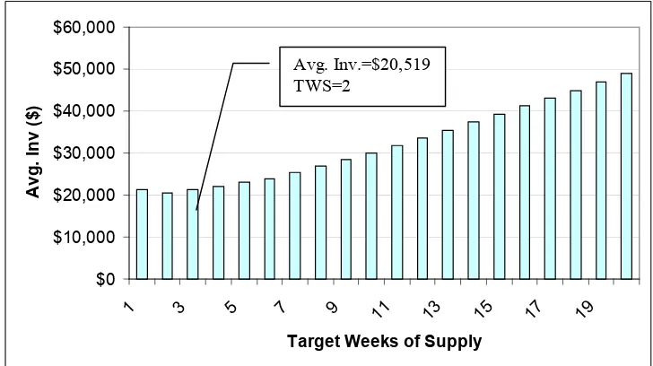
FIGURE 4.6 AVG. INV. WITH TWS, NO PRESENTATION STOCK...67
FIGURE 4.7 SL WITH TWS, NO PRESENTATION STOCK...67
FIGURE 5.1 PARETO FRONTIER WITH TWO OBJECTIVES...76
FIGURE 5.2 FAST NON-DOMINATING SORTING...78
FIGURE 5.3 CROWDING DISTANCE FUNCTION...79
FIGURE 5.4 COMPARISON OPERATOR ³N...79
FIGURE 5.5 NSGA-II MAIN ALGORITHM...80
FIGURE 5.6 PARETO OPTIMAL FRONTIER WITH 300 GENERATIONS...83
FIGURE 5.7 PARETO OPTIMAL FRONTIER WITH 500 GENERATIONS...84
LIST OF TABLES
TABLE 2.1 RANGE FOR THE VARIABLES USED IN THE EXPERIMENTATION...25
TABLE 2.2 PARAMETERS USED IN THE GA EXPERIMENTATION...25
TABLE 2.3 EXPERIMENTAL DESIGN...26
TABLE 2.4 RESULTS OF GA OPTIMIZATION AND RANDOM-START PROCEDURE...29
TABLE 3.1 PARAMETERS USED IN THE GA EXPERIMENTS...36
TABLE 3.2 RANGE FOR THE DECISION VARIABLES...36
TABLE 3.3 EXPERIMENTAL DESIGN FOR EXPERIMENT SET 1...37
TABLE 3.4 ANOVA TABLE FOR GMROILS FOR EXPERIMENT SET 1...39
TABLE 3.5 SUMMARY OF MULTIPLE REGRESSION WITH ONLY MAIN EFFECTS...41
TABLE 3.6 ANOVA TABLE FOR MULTIVARIATE REGRESSION ON INIT_DROP% MODEL 2 SET 1 ...41
TABLE 3.7 PARAMETER ESTIMATES FOR MULTIVARIATE REGRESSION ON INIT_DROP% MODEL 2 SET 1 ...41
TABLE 3.8 ANOVA TABLE FOR MULTIVARIATE REGRESSION ON NO_OF_REOR MODEL 2 SET 1 ...42
TABLE 3.9 PARAMETER ESTIMATES FOR MULTIVARIATE REGRESSION ON NO_OF_REOR MODEL 2 SET 1 ...42
TABLE 3.10 ANOVA TABLE FOR MULTIVARIATE REGRESSION ON START_WK MODEL 2 SET 1 ...42
TABLE 3.11 PARAMETER ESTIMATES FOR MULTIVARIATE REGRESSION ON START_WK MODEL 2 SET 1 ...42
TABLE 3.12 EXPERIMENTAL DESIGN FOR SET 2...43
TABLE 3.13 ANOVA TABLE FOR GMROILS FOR EXPERIMENT SET 2...45
TABLE 3.14 ANOVA TABLE FOR MULTIVARIATE REGRESSION ON INIT_DROP% MODEL 3 SET 2 ...46
TABLE 3.15 PARAMETER ESTIMATES FOR MULTIVARIATE REGRESSION ON INIT_DROP% MODEL 3 SET 2 ...47
TABLE 3.16 ANOVA TABLE FOR MULTIVARIATE REGRESSION ON NO_OF_REOR MODEL 3 SET 2 ...47
TABLE 3.17 PARAMETER ESTIMATES FOR MULTIVARIATE REGRESSION ON NO_OF_REOR MODEL 3 SET 2 ...47
TABLE 3.18 ANOVA TABLE FOR MULTIVARIATE REGRESSION ON START_WK MODEL 3 SET 2 ...48
TABLE 3.19 PARAMETER ESTIMATES FOR MULTIVARIATE REGRESSION ON START_WK MODEL 3 SET 2 ...48
TABLE 4.1 RANGE FOR THE DECISION VARIABLES...59
TABLE 4.2 PARAMETER VALUES FOR THE ADAPTIVE PENALTY METHOD...61
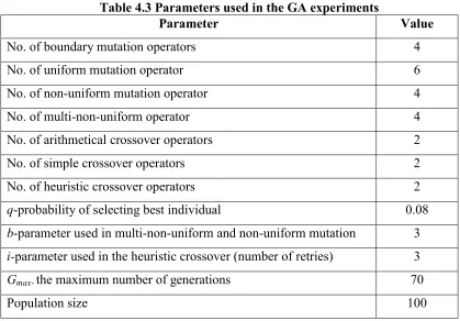
TABLE 4.3 PARAMETERS USED IN GA EXPERIMENTS...61
TABLE 4.4 EXPERIMENTAL DESIGN FOR SET 2...61
TABLE 4.5 BEST SOLUTIONS BY NO. OF CATEGORY WITH DISCRETE CUTOFF POINTS...70
TABLE 4.6 OPTIMAL SOLUTIONS OBTAINED BY CONSTRAINED GA WITH PRE-DETERMINED PRESENTATIONS STOCK....72
CHAPTER 1
INTRODUCTION
Nowadays, almost all companies try to concentrate their business on the activities that they know best. These activities are referred to as the core competencies of a company. However by concentrating efforts on core competencies, all other activities had to be outsourced. Therefore quality of products and services, and customer satisfaction are functions of performances of the firms involved in the process. The greatest challenge for a successful business is then the integration of the separate business units and the coordination of materials and information among these companies.
Supply Chain Managament (SCM), is best defined as “the task of integrating organizational units along a supply chain and coordinating materials, information and financial flows in order to fulfill (ultimate) customer demands with the aim of improving competitiveness of the supply chain as a whole.” (Stadler and Kilger, 2000). In a broader sense, a supply chain consists of two or more legally separated organizations, linked by materials, information and financial flows. These organizational units might be firms producing parts, end products, service providers or end customers.
The potential for impressive gain from coordinating organizational units and integrating information flows and planning efforts along a supply chain has been realized in the recent decade:
· IBM applied its Asset Management Tool, which consists of analytical performance optimization and simulation, to its personal systems divisions. The application resulted savings in material costs and price-protection expenses that added up to $750 million in 1998 (Lin et al., 2000).
· BASF introduced vendor managed inventory with 5 key customers in its textile colors division. The advanced planning system used enabled ASF to raise the fill rate of the customer’s inventory to almost 100%. BASF was able to generate less costly production and transportation schedules while the customers eliminated safety stocks completely (Grupp, 1998).
· Hewlett-Packard (HP) used different inventory models to analyze the effect of different locations and inventories within its supply chains. The analysis convinced HP to adopt a modular design and postpone its deskjet printers. As a result, they were able to reach a reduction of 25% in the supply costs of deskjet printers. (Lee & Billington, 1995).
The main objective of SCM is to increase competitiveness. But no single unit can be held responsible for competitiveness of a product or service. The supply chain as a whole is responsible. For this reason, the competition in the marketplace has inevitably shifted from being between single companies to being between supply chains. A company and its success is now defined by its supply chains.
One can approach SCM problems from one of the many facets that it has. In this research, we concentrate our efforts on the effective operation of supply chains. From an operational point of view, a supply chain can be thought of as made up by three major components: sourcing and procurement, manufacturing and distribution, and inventory disposal. This dissertation is focused on sourcing component of a supply chain.
materials and services acquired from outside companies. Sourcing is an area where there is vast potential for adding value. This is the reason why more and more companies include strategic sourcing as a core competency (Tyndall et al, 1998).
Increasing pressure and requirements for responding to customer demand in a timely basis have been dealt by choosing the lowest cost alternative and trying to offset for the long lead-time by forecast based methods. Recent decades have opened the gates for sourcing products and materials off-shore, encouraged by substantial cost savings. Rarely have the consequences of significantly longer lead-times on total chain performance been considered even though the effects might be severe. Usually, the time it takes to convert material to products and moving them to marketplace is invariably longer than the time customers are prepared to wait. This so called “lead-time gap” (Fernie and Sparks, 1999, pp.94) was filled with forecast-based inventory. However, with sourcing off-shore with long lead-times and almost no flexibility, the company cannot ensure that the product will be available when the customer wants it. The problem with keeping this kind of inventory is that the inventory is usually wrong in the sense that sizes, styles, and colors are not those actually demanded.
The remainder of this dissertation is organized as follows: Chapter 2 mentions the deficiencies in some of the traditional supply chain performance measures, and also talks in detail about a new performance measure, GMROILS. A GA based simulation-optimization methodology to solve sourcing decisions in supply chains is also introduced. The proposed methodology is tested on a scenario dealing with replenishment of a seasonal item to a single retailer.
Chapter 3 consists of experimentation to test the effectiveness of the proposed methodology. The experimental designs aim to find effects of some factors of interest on the optimal performance as well as ways to determine levels of decision variables to set that will achieve the best performance under a wide range of scenarios. ANOVA, multivariate regression and neural networks are used for determining the factors important in determining optimal solution as well as for determining levels of the decision variables to obtain optimal performance for any given parameter setting.
Chapter 4 introduces the constrained GA optimizer. We first run the same experimental design in chapter 3 to test the new performance measure GMROILS and the findings about the optimal settings for decision variables while the second part of chapter 4 is a case study. The constrained GA is used to find optimal sourcing settings for a basic product with 420 SKUs. The constrained GA performs successfully and the results from the experiments shed light on some insights into the characteristics of the best sourcing practices.
CHAPTER 2
OPTIMIZATION OF SOURCING
DECISIONS FOR A SEASONAL
ITEM
This chapter describes the proposed genetic algorithm based simulation optimization methodology. First the problem is defined. Available literature on related topics is reviewed in 2.2. The details of the proposed methodology along with the definition and justification of a new performance measure, GMROILS, are given in section 2.3. Results from the experimentation with the proposed methodology and the new performance measure are presented in section 2.4. The chapter ends with some concluding remarks in 2.5.
2.1
INTRODUCTION
decisions normally depend solely on minimizing the cost of goods, and production and distribution decisions often consider only maximizing throughput while minimizing production (unit) costs without any consideration for high inventory levels or long lead-times. This situation does not only create as many different business plans as the number of organizational units but it also decreases the overall gain of the players in the supply chain significantly. A company’s success or survival against these challenges does not come from isolated efforts in different companies and/or departments within the same organization, but through coordinated efforts between different organizational units as well as separate organizations. Supply chain management is the effective coordination and integration of different organizations with different objectives towards a common goal. The great potential for improvement in these objectives through effective supply chain management mechanisms has recently been realized (Karabakal et al., 2000; Lyon et al., 2001; Hahn et al., 2000).
A supply chain, from an operations perspective, has three components: sourcing or procurement, manufacturing and distribution, and inventory disposal. The focus of this chapter is on decision making in the sourcing component of a supply chain. In particular, we develop a simulation-based, genetic procedure for determining optimal settings for controllable inputs.
Sourcing decisions have a large impact on manufacturing and distribution and inventory disposal in a supply chain as well. Therefore, sourcing and procurement decisions directly affect the efficiency of the entire supply chain. Because sourcing decisions include the supplier, which is usually a separate company, these decisions are much more rigid than manufacturing, distribution, and inventory disposal decisions. Whereas manufacturing and inventory disposal decisions might be internal to a company most of the time and therefore easier to change or modify, sourcing decisions that include outside companies will be hard to change due to contracts and agreements.
excessive inventory, poor customer service, lost revenues, and missed production schedules. In a typical supply chain for a consumer product, even when consumer demand does not seem to vary much over time, there is a significant variance in the retailer’s orders to the manufacturer. The variability increases as we move up to the supply chain. Procter & Gamble (P&G) noticed this effect when the logistic executives examined the order patterns for their popular diaper brand, Pampers. Although sales were fluctuating, the variability in retail stores was certainly not excessive. However, the variability in the orders from the distributors was considerably higher. When the orders of materials to their suppliers, such as 3M, were analyzed, the variability was even greater. Sourcing decisions play an important role in limiting or contributing to the bullwhip effect. Figure 2.1, modified from Lee et al. (1997), shows the bullwhip effect in a serial supply chain with four members (Retailer, Wholesaler, Manufacturer, and Supplier). Consumer Sales 0 5 10 15 20 Time
Retailer's Order to Wholesaler
0 5 10 15 20
1 3 5 7 9 11 13 15 17 19 21 Time
Order Quanti
ty
Wholesaler's Order's to Manufacturer
0 5 10 15 20 Time
Manufacturer's Order to Supplier
0 5 10 15 20 Time
Figure 2.1 Increasing Variability of Orders up to the Supply Chain
shipping, the complexities of modeling the individual entities, the stochastic nature of the demands, etc. Because of these complexities, very few analytical models exist except for simplified versions of the problem, which often are based on limiting assumptions. Even if the analytical forms do exist, it is very difficult to solve these models using traditional search methods like linear programming, differentiation, or even local gradient-based methods owing to the fact that most of the models are discrete, non-linear and/or multi-modal. Therefore, heuristic or computational methods are required to even determine good solutions.
Computer simulation is a methodology that can be used to directly model the complexities of the entire supply chain without as many limiting assumptions. Computer simulation can be used to describe and analyze the behavior of a supply chain and can aid in the design/control of the supply chain through evaluation of “what if” questions (i.e., What if we source our product from these two suppliers? or What if we drop ship 20% of the estimated demand from one supplier and quick replenish every four weeks from this supplier?). However, other practical questions (such as Which combination of suppliers is best? and What is the best sourcing strategy under these conditions?) seek optimum values for the decisions variables of the system for the one or more performance measures. In this case, the simulation model can be thought of as the objective function and/or constraint functions in optimizing these complex stochastic systems.
Using simulation in the optimization process presents several challenges. First, there is no analytical expression of the objective function, which eliminates differentiation, or exact calculation of local gradients. Further, the stochastic nature of the simulation causes problems because given a set of deterministic decision variables, the performance measure is not crisp but rather is described by a probability distribution. Simulation programs are typically computationally more expensive to evaluate than analytical functions. Therefore, the efficiency of the optimization algorithms is more crucial.
merchandise from a supplier for a retailer. To test the technique, the Sourcing
SimulatorÒ (Hunter, King and Lowson, 2002; Hunter, King, and Nuttle, 1992, 1996; King, and Nuttle, 1999; Lowson, King and Hunter, 1999; Nuttle, King, and Hunter, 1991) is used as the simulation tool/evaluation function. The Sourcing Simulator can evaluate a sourcing strategy for a retailer for a given set of inputs. The tool is expanded using the optimization methodology to find the best scenario for a given performance measure/measures.
2.2 RELATED LITERATURE
The literature review in this section is divided into four sub-sections. First, a review of performance measures for sourcing problems is presented. Section 2.2.2 gives detailed information and review of literature on the sourcing simulator. In Section 2.2.3, a general overview of simulation-optimization techniques is presented. Lastly, section 2.2.4 introduces genetic algorithms and provides the motivations behind using genetic algorithms in this research.
2.2.1
Performance Measures for Supply Chains
Gross Margin (GM) is a widely-used supply chain performance measure. It is calculated using the following formula and takes into account the profitability of the supply chain.
Gross Margin Total Revenue Cost of Goods
Total Revenue Number of units purchased Wholesale cost/unit
=
-= - ´
GM is a measure of revenue only. It neither takes into effect the cost of carrying inventory nor relates to the chain’s customer service level. In an effort to improve GM, Gross Margin Return on Investment (GMROI) adjusts GM for the average inventory held over the period and is an effective measure that takes into account the money earned and inventory held. It is calculated using the following formula:
GM GMROI
Avg. Inv (Wholesale cost/unit)
=
´
2.2.2
The Sourcing Simulator
The Sourcing Simulator is a stochastic simulation model for the consumer product retailing process developed by Nuttle, King and Hunter (1991). The model allows investigation of the effects of alternative retailing procedures on financial and other performance measures for a retail store. The value of the model lies in the fact that it captures the random nature of consumer behavior at the retail store within a robust framework that allows investigation of buyer strategies. Consumer arrivals at the retail store are modeled as a time-dependent Poisson process. The rate each week is based on a specified seasonal arrival pattern. The model tracks the inventory by stock keeping unit (SKU). A forecast of consumer demand is expressed in terms of customer volume, SKU mix and presumed seasonality. The model assumes that this forecast is in error. This error is specified as a volume error, SKU mix error, and actual seasonality.
It models alternative mechanisms for supplying product to a retail store. The model tracks the inventory of a line of product offered in a range of SKUs. The store sets up an initial inventory to start the selling season according to the store buyer’s plan. Customers arrive at the store and attempt to purchase garments. For a particular customer, if the desired SKU is in stock, a sale is recorded and inventory decremented. If the SKU is out of stock, a stockout is recorded. In either case the customer may look for another item with certain probabilities. Periodically the store may issue replenishment orders on the vendor. Replenishment may be based upon the original buyer’s plan or may reflect the use of actual Point-of-Sale (POS) data. In this way the selling season is played out and performance statistics are computed.
reduction. First, customer arrivals to the store increase proportional to the reduction in price based on price elasticity. Second, the probability that a customer selects an alternate SKU after encountering a stockout increases.
Nuttle, King and Hunter (1991) present several case studies for illustration of re-estimation of demand and quick response (QR) versus traditional retail practice. The case studies showed clearly that useful information can be made available very early in the season both to the buyer and, if shared, to the apparel manufacturer and textile producer, to whom lead-time is critical by use of demand re-estimation. Comparisons of performance parameters for both traditional and QR procedures show clearly the superiority of the QR methods.
Hunter, King, and Nuttle (1992) expanded the capability of the Sourcing Simulator to include a responsive fabric-supply component by modeling the manufacturer portion to form an apparel-supply chain system for QR retailing. In-season apparel shop order releases are calculated weekly depending on retail orders received but not yet shipped, backorders, work-in-process, finished inventory, availability of fabric and constrained on minimum release batch for individual SKUs, maximum number of SKUs in a shop order and shop capacity. Weekly, in-season fabric reorders are calculated based on net fabric requirements from apparel shop orders. The order size is limited by the allocated weekly apparel shop capacity, as there is no need to carry fabric that cannot be used. Results obtained using the simulation model are also presented in the paper. They conclude that apparel-manufacturing systems exist that allow retailer performance to come very close to the case with a perfect supply by the vendor.
Hunter, King and Nuttle (1996) explore the applicability and benefits of QR compared to traditional retailing procedures. They extend their previous work and present results on the impact of assortment error, volume error, price markdowns, reorder lead-time, bi-weekly reorders, season length, number of SKUs on performance.
2.2.3
Simulation Optimization
Law and McComas (2000) define simulation optimization as the “orchestration of the simulation of a sequence of system configurations (each configuration corresponds to particular settings of the decision variables (factors)) so that a system configuration is eventually obtained that provides an optimal or near optimal solution.” Several excellent survey papers have been written on simulation optimization techniques and procedures. Swisher et al. (2000) Androdottir (1998a, 1998b), Carson and Maria (1997) and Fu (1994a, 1994b) present reviews of simulation optimization techniques both for continuous and discrete decision variables. This section is intended to give a brief overview of simulation-optimization techniques. The reader is encouraged to refer to the survey articles mentioned above or to the articles specified in the corresponding sections below for detailed information on a specific technique. A detailed description of available simulation based optimization packages, their vendors and the heuristic search procedures that they use may be found in Law and Kelton (2000), section 12.6.
Simulation optimization techniques and procedures can be summarized in two main categories based on the characteristics of the decision space: Continuous versus discrete input spaces.
2.2.3.1 Continuous Input Parameter Methods
found in the literature include perturbation analysis, harmonic analysis, likelihood ratios and score functions. Response surface methodology and stochastic counterpart are some of the other gradient-based simulation optimization techniques besides stochastic approximation. The reader is referred to Swisher et al. (2000) for a detailed discussion on the literature on gradient-based simulation optimization techniques.
Direct methods: Methods in this category include Nelder-Mead simplex method, Hooke and Jeeves method, and sample path method. For a detailed review of direct simulation optimization techniques, the reader is referred to Swisher et al. (2000) and Andradottir (1998a).
2.2.3.2 Discrete Input Parameter Methods
The feasible region is discrete. When the size of the feasible region is relatively small, ranking and selection, multiple comparison procedures are used in literature (Goldsman and Nelson, 1994, 1998; Bechhofer et al., 1995; Hsu, 1996). When the size of the feasible region is infinite or very large, ordinal optimization (Ho et al., 1992), and metaheuristics such as simulated annealing (Fleischer, 1995), tabu search (Glover and Laguna, 1997) and genetic algorithms (Tompkins and Azadivar, 1995; Liepens and Hilliard, 1989) are among the methods found in the literature.
The most important issue in simulation optimization has been the limitation that arises out of inability to be able to simulate more than a fraction of the usually very large number of solutions. An effective search mechanism to guide a series of simulations to produce optimal or near-optimal solutions is needed. Genetic algorithms offer an efficient approach for these problems.
2.2.4
Genetic Algorithms
Genetic algorithms (GAs) are a powerful set of stochastic global search techniques that have been shown to produce very good results for a wide class of problems. GAs can find good solutions to linear and nonlinear problems by simultaneously exploring multiple regions of the solution space and exponentially exploiting promising areas through mutation, crossover and selection operations (Michalewicz, 1994). In general, the fittest individuals of any population are more likely to reproduce and survive to the next generation, therefore improving successive generations. However, some of the inferior individuals can, by chance, survive and also reproduce. Unlike many other optimization techniques, GAs do not make strong assumptions about the form of the objective function (Michalewicz, 1994). Traditional search techniques use characteristics of the problem (objective function) to determine the next sampling point (e.g., gradients, Hessians, linearity, and continuity), however, the next sampled points in genetic algorithms are determined based on stochastic sampling/decision rules, rather than a set of deterministic decision rules. Therefore, evaluation functions of many forms can be used, subject to the minimal requirement that the function can map the population into a totally ordered set. A more complete discussion of GAs, including extensions to the general algorithm and related topics, can be found in books by Davis (1991),Goldberg (1989), Holland (1975), and Michalewicz (1994).
Each solution (individual) in the population of a genetic algorithm is described by its chromosome representation, which is a vector of variables. The first step in a GA (as seen in Figure 2.2) is to initialize the population. This can be done either randomly or by seeding. Once the initial population is generated, each individual, i, is evaluated using the objective function to determine its fitness or value, Fi. To generate the next
crossover, two new individuals are reproduced from two parents by combining the parent chromosomes. In mutation, randomly selected individuals from the population undergo changes in chromosomes randomly. To complete the new population, a subset (arbitrary or otherwise) of the old population is added to the new population. The general genetic algorithm is summarized in Figure 2.2.
1. Supply a population P0 of N individuals and respective function values.
2. i ß1
3. Piß selection_function(Pi-1)
4. Piß reproduction_function(Pi)
5. Evaluate(Pi)
6. i ß i+1
7. Repeat steps 3-6 until some termination is reached 8. Report best solution found
Figure 2.2 Generic Genetic Algorithm Procedure
2.2.4.1 Differences Between Genetic Algorithms and Traditional Methods
In complex problems such as sourcing in supply chains, it is usually impossible to define one functional form that will, upon evaluation, give a measure of goodness for the solution. Simulation, in these cases, is often the only way to evaluate a solution. Therefore, a proposed solution methodology must be a simulation optimization technique. Although genetic algorithms usually rely on some sort of functional form to evaluate each individual (solution), there have been a limited number of successful studies in recent years on manufacturing systems using GAs in simulation optimization (Bowden and Neppalli, 1995; Tompkins and Azadivar, 1995). Since genetic algorithms rely on the premise of selection and survival of the fittest, it actually makes sense to simulate the solution each individual corresponds to. Also, GAs are able to operate relatively unaffected by the noise from observations from a simulation. Since stochastic simulation generates noisy responses, GAs are a good solution method candidate for simulation-optimization (Goldberg, 1989; Tompkins and Azadivar, 1995).
In general, simulation-optimization techniques require the decision variables to be quantitative, i.e., the values of the decision variables must be ordered. But in a wide variety of production systems problems, such as scheduling, planning, supply chain management etc., qualitative variables do exist and have to be decided upon. A decision variable such as queuing discipline might take values such as FIFO, LIFO, etc. that have no order and therefore quantitative search methods are not suitable for optimization of such variables. Other possible variables in sourcing models may include the decision to have markdowns or not or an information sharing policy between the supplier and the retailer, etc. Also, changes in quantitative variables generally do not cause any change to the framework of the system, whereas changes in qualitative variables allow for changes in the physical and logical structure of the system. GAs have the advantage of being able to handle not only quantitative but also qualitative variables (Tompkins and Azadivar, 1995, 1999).
algorithms have shown to be a very good alternative for handling multi-objective problems in many studies including Bussaca et al. (2001) and Li et al. (2000). Genetic algorithms also have the advantage of being able to work efficiently both with continuous and integer variables.
Considered altogether, genetic algorithms offer a more robust, efficient search technique suitable for large combinatorial problems. These differences are the main motivations behind the use of genetic algorithms in this research.
2.3
APPROACH AND METHODOLOGY
The supply chain optimization problem considered in this chapter is very complex, and the solution space is not easy to search because of the landscape and the size of the space. For the instance of the problem defined in section 2.4, which has only 5 decision variables, the size of the solution space can be calculated to be 18,998,100. Even when the solution space size is not a large number, each one of these solution vectors has to be evaluated using the simulator, which is time consuming. Therefore, the large solution space needs to be explored efficiently. The solution space is also likely to have many local optima, which limits the effectiveness of local or neighborhood searches. The characteristics of the solution space can change very easily with different instances of the same type of problem. Therefore, the proposed solution technique must be relatively robust as well.
2.3.1
Solution Technique
In building a genetic algorithm methodology to solve the supply chain sourcing problem, six fundamental issues that affect the performance of the GA must be addressed: chromosome representation, initialization of the population, selection strategy, genetic operators, termination criteria, and evaluation measures. In the following subsections, these issues are introduced and described specifically for the proposed genetic algorithm.
2.3.1.1 Chromosome Representation
For any GA, a chromosome representation is needed to describe each individual in the population. Chromosome representation determines how the problem is structured in the GA, as well as the genetic operators that can be used. For the sourcing decision, the chromosome representation in this case is fairly straightforward. An individual is kept as an array of size 5, where each cell corresponds to a decision variable (as seen in figure 2.3). The five decision variables are:
1. Initial Drop: The percentage of total order for season that is purchased pre-season. For traditional sourcing, this variable will be 100% and can range from 0 to 100% in the GA.
2. Number of Reorders: The number of in-season reorders during the season. The maximum number of reorders is limited by the fact that no delivery is allowed during the last 2 weeks of the season.
3. Reorder Start: Week in the season at which reorders start.
4. Lead Time: In season reorder lead-time in weeks. Range of lead-times can be any integer from 0 up to the half of the season length.
5. Minimum Order/SKU: Minimum order quantity per SKU. This variable is especially meaningful when quantity discounts are introduced and can range from one to 60.
Initial drop
Number of Reorders
Reorder Start Week
Lead-time Minimum. Order/SKU
Figure 2.3 Sample Chromosome
Notice that not all combinations of the decision variables constitute a feasible solution. For this reason, infeasible solutions are repaired using a repair function before they are evaluated by the Sourcing Simulator. This repair procedure is presented in appendix 1 in detail.
2.3.1.2 Initialization of the Population
The initial population is formed randomly based on the upper and lower bound for each of the decision variables in a chromosome using a uniform distribution.
2.3.1.3 Selection Strategy
Selection of parents to produce successive generations is very important in driving the search. The goal is to give more chance to the “fittest” individuals to be selected. For each selection scheme, probabilities are assigned to the individuals. The better individuals have higher probabilities. A normalized geometric ranking scheme is used for the proposed genetic algorithm in this chapter. Individuals are first ranked from best to worst according to their fitness values. Then each individual is assigned a probability based on a normalized or truncated geometric distribution (Joines and Houck, 1994).
2.3.1.4 Genetic Operators
Reproduction is carried out by application of genetic operators on selected parents from the population. Four mutation and three crossover operators are used. The boundary mutation operator randomly selects a variable, vi, from a parent chromosome and sets it
either to its lower or upper bound. The uniform mutation operator randomly selects a variable from a parent and changes its value in its range based on a uniform probability distribution
) (a b r a
-where (0,1). between number random uniform variable of bound upper variable of bound lower 1 = = = r i b i a i i
The non-uniform mutation operator randomly selects a random variable in a parent, vi, to a random displacement from the distribution described below. This operator needs
two uniform (0,1) random variables, r1 and r2. The first random number, r1, is used to
determine the direction of the displacement and the second random number, r2, is used to
generate the magnitude of the displacement
î í ì -< -+ = otherwise, ) ( ) ( , 5 . 0 if ) ( ) ( 1 G f a v v r G f v b v v i i i i i i i where 2 2 max 2 max
( ) (1 )
uniform random number between (0,1) current generation number
maximum number of generations. G
f G r G r G G = -= = =
In early generations, this operator is similar to uniform mutation operator. But as the generation number, G, increases, the distribution gets narrower, increasing exploitation of the local solution.
2.3.1.5 Termination Criteria
The GA is terminated after a specified number of generations. This number is set as one hundred for all of the runs in this study.
2.3.1.6 Evaluation Measure
Genetic algorithms rely on the simple premise of using natural selection as a means of solution elimination. The objective function is the driving force of the GA search. In this research, instead of performing an analytical function evaluation, each solution is simulated to determine its performance. Each solution is evaluated via the Sourcing Simulator. The performance measure in the next section is used to evaluate the solution.
2.3.2
GMROILS : A New Performance Measure
It was mentioned in section 2.2 the limitations of the typically-used performance measures. In this section, a new performance measure, Gross Margin Return on Investment-Lost Sales (GMROILS) is developed. GMROI incorporates a tradeoff between reducing inventory and making more money. However, it does not take into account the customer service level. Clearly, minimizing the number of lost sales will lead to increased customer service. Since lost sales are not typically observed and measured, an estimation of lost sales is used. Lost sales in any week can be estimated using the following rules. In any week, if inventory of a SKU runs out, it is assumed that it happened in the middle of the week and therefore half of the estimated demand in that week for that item is lost. If there was no inventory for a SKU during the entire week, then all of the estimated demand for that SKU in that week is lost.
sales. Also, the lost sale estimates are added to calculation of average inventory assuming that they would be purchased at the latest week possible to be ready in the week in which they occurred. Based on this, GMROILS is calculated as follows:
1
1
S*r ( ) ( )
( ) 2 W i i W i i i
N S l c N L
GMROILS L I c W = = + - - + = + ´
å
å
where= total number of units purchased throughout the season = Season length
= total number of units sold through the season = estimated lost sales in week
= retail price/unit = i N W S L i r
c wholesale cost/unit = liquidation price/unit
= Average inventory in period in $i
l
I i
2.4
EXPERIMENTATION
In order to test this methodology the Sourcing Simulator source code was linked with a GA solution technique. The implementation of the genetic algorithm was done in Matlab using GAOT (Genetic Algorithm Optimization Toolbox) developed by Houck et al. (1995).
Table 2.1 Range for the decision variables used in experimentation Decision Variable Lower Bound Upper Bound
Initial Drop Percentage(%) 0 100
Number of Reorders 0 18
Reorder Start Week 1 18
Lead-Time 0 10
Min. Ord. Quan./SKU 1 60
Table 2.2 Parameters used in the GA experiments
Parameter Value
No. of boundary mutation operators 4
No. of uniform mutation operator 6
No. of non-uniform mutation operator 4
No. of multi-non-uniform operator 4
No. of arithmetical crossover operators 2
No. of simple crossover operators 2
No. of heuristic crossover operators 2
q-probability of selecting best individual 0.08 b-parameter used in multi-non-uniform and non-uniform mutation 3 i-parameter used in the heuristic crossover (number of retries) 3
Gmax- the maximum number of generations 100
Population size 100
corresponding GA replication. On the average, the GA performs approximately only 1,850 evaluations. Since the GA only performs significantly fewer evaluations, we feel this is more than fair to random evaluation procedure.
To test the performance of the proposed solution technique, three parameters were varied for three levels, forming the experimental design in Table 2.3.
Table 2.3 Experimental Design
SKU Mix Error Number of SKUs Season Length
Level 1 Low=20/20/10 Low=18 10 Periods
Level 2 Medium=40/40/20 Medium=48 15 Periods Level 3 High=60/60/40 High=80 20 Periods
The assortment error triplet (A/B/C) is a measure of the difference between the forecast and actual assortment preferences for style, color, and size (Nuttle et al., 1991). See Appendix 3 for the description of this measure.
To fully explore the effects of the parameters chosen and test the performance of the GA technique, 27 experiments were carried out. Each experiment corresponds to a combination of levels of the three parameters of the experimental design. Table 2.4 presents the results of optimization for each of the 27 experiments and comparisons with the results of the random-start procedure. Each row of table is the average over the 10 replications made.
To see if the differences between the results of the GA optimization and random-start procedure are statistically significant, a t-test is performed. The last column in table 2.4 gives the t values for each row for the differences between the results of GA method and
the random-start procedure. tcritical is 1.734 at a = 0.05 and 3.922 at a = 0.0005. The
differences between the results from GA method and from random-start method are statistically significant for all experiments at both levels.
GA method provides substantially better results than random-start procedure for all of the 27 experiments showing that it will be useful over a wide range of scenarios.
2.5
DISCUSSION
In this chapter, we consider the problem of optimizing sourcing decisions in a supply chain. A genetic algorithm-based procedure with complex evaluations is proposed for this purpose. A new performance measure is developed that combines measures of revenue, inventory and customer service. The proposed methodology is tested on a single supplier-single retailer 2-stage supply chain with multiple items (SKUs) with stochastic demand and substitutability. Experimentation shows that genetic algorithms with complex evaluations using the new performance measure provide superior solutions over a random-start heuristic over a wide range of scenarios. The GA method performs significantly better under all levels of number of SKUs and SKU mix errors and season length.
Finally, we list some observations made on the optimal solutions from the experimentation along with suggestions for future work:
· For all of the experiments, the ranking of best GMROILS achieved by the GA for different season lengths is as follows: GMROILS20 Periods > GMROILS15 Periods >
GMROILS10 Periods. GMROILS tries to minimize average inventory and lost sales and
periods, there is just not as much time to use POS data as effectively to estimate real demand good enough and reorder accordingly. Since the performance of the optimization technique improves with longer season length, it might be worthwhile to look at basic items as well.
· Looking at the results, one can also see that performance is better in general with low number of SKUs compared to higher number of SKUs. This is probably due to the fact that when the number of SKUs increase, the demand per SKU decrease as the total volume is fixed no matter what the number of SKUs is. When the demand per SKU decrease, the probability of having lost sales increases, which in turn deteriorates performance.
· The initial drop percentage for the optimal solutions usually range from 10% to 20%. The optimal values of the lead-time are usually chosen to be the minimum value possible. Optimally, reordering starts either in the first week or second week. The combination of the lead-time and reorder start week seems to be arranged so as to maximize the number of the reorders. Remember that no reorder is allowed to arrive last 2 weeks of the season. Therefore, the strategy is set to choose the low lead time, early start and as many reorders as possible. The advantage gained from additional reorders outweighs reordering cost.
· The experimentation in this chapter is assumes a mid-peak seasonality pattern. Although quite common, mid-peak is not the only seasonality pattern for seasonal products. Additional experimentation must be done to evaluate the performance of the optimization technique with other seasonality patterns.
Table 2.4 Results of GA optimization and random-start procedure
Experiment
No SKU MixError Number ofSKUs Season Length(Periods) GMROILSGA Best Of GA bestStd. Dev. Start GMROILSBest Random Std. Dev. Of BestRandom Start GA Best- Randomstart best improvement t valueGA's %
1 Low Low 10 5.36 0.4105 4.26 0.5610 1.10 25.86% 8.08
2 Low Low 15 6.45 0.3337 5.21 0.5478 1.23 23.67% 9.81
3 Low Low 20 6.77 0.0169 5.94 0.3263 0.83 14.00% 12.98
4 Medium Low 10 4.09 0.2760 3.62 0.3161 0.47 13.05% 5.74
5 Medium Low 15 5.26 0.6720 4.62 0.4778 0.64 13.75% 3.93
6 Medium Low 20 6.25 0.1050 5.29 0.2959 0.96 18.07% 15.53
7 High Low 10 4.55 0.0263 3.41 0.5320 1.14 33.51% 10.94
8 High Low 15 5.77 0.2868 4.29 0.3850 1.48 34.63% 15.77
9 High Low 20 5.81 0.0377 4.67 0.2992 1.14 24.45% 19.29
10 Low Medium 10 4.69 0.0325 3.72 0.4629 0.96 25.91% 10.60
11 Low Medium 15 5.92 0.0166 4.36 0.4729 1.56 35.77% 16.79
12 Low Medium 20 5.84 0.0381 5.24 0.1985 0.60 11.35% 15.02
13 Medium Medium 10 4.34 0.0000 3.27 0.5882 1.07 32.87% 9.31
14 Medium Medium 15 5.35 0.0595 3.83 0.4646 1.52 39.58% 16.52
15 Medium Medium 20 5.36 0.1322 4.50 0.2261 0.85 18.94% 16.61
16 High Medium 10 3.42 0.0085 2.55 0.5433 0.87 34.30% 8.20
17 High Medium 15 4.98 0.0195 3.35 0.3998 1.64 49.01% 20.89
18 High Medium 20 5.47 0.0000 4.13 0.3510 1.34 32.51% 19.50
19 Low High 10 2.91 0.0630 2.38 0.2406 0.53 22.25% 10.87
20 Low High 15 3.57 0.0822 2.76 0.3254 0.81 29.47% 12.36
21 Low High 20 3.61 0.0453 3.26 0.2001 0.35 10.69% 8.65
22 Medium High 10 2.87 0.1228 2.19 0.3600 0.69 31.44% 9.21
23 Medium High 15 3.99 0.0903 2.64 0.3446 1.35 51.07% 19.32
24 Medium High 20 4.34 0.0000 3.19 0.2418 1.16 36.33% 24.42
25 High High 10 2.72 0.0041 2.07 0.3723 0.65 31.64% 8.96
26 High High 15 3.68 0.0000 2.51 0.2698 1.17 46.50% 22.07
CHAPTER 3
ANALYSIS OF OPTIMAL
SOURCING DECISIONS FOR
SEASONAL ITEMS
This chapter builds on the proposed optimization method in chapter 2. The genetic algorithm (GA) based simulation-optimization methodology is applied to two separate experimental designs with the hope of providing insight into effects of some factors on optimal performance and optimal sourcing strategies.
3.1 INTRODUCTION
Today, companies no longer can focus only on themselves. The road to success for companies goes through the success of their entire supply chain. Survival in today’s marketplace depends heavily on the coordinated efforts among different organizational units as well as outside organizations. Supply chain management is the effective coordination and integration of different organizations with different objectives toward a common goal. Karabakal et al. (2000), Lyon et al. (2001), Hahn et al. (2000) are just a few of the many publications that drew attention to the potential for improvement through effective supply chain management mechanisms.
In this chapter, two sets of experimentation is carried out with the proposed GA based simulation-optimization methodology to find out the potential improvements achievable through good decision-making for sourcing in supply chains.
service levels are considered. Sourcing decisions have a large impact on manufacturing, inventory disposal, and distribution in a supply chain. Therefore, sourcing decisions directly affect the efficiency of the whole supply chain. For this reason, sound decision making procedures and strategies for sourcing can be the key to the survival and success in marketplace.
Lee, Padmanabhan and Whang (1997) first drew attention to the concept of “bullwhip effect.” Distorted information from one end of the supply chain to the other can cause inefficiencies like inventory pile-ups, low service levels, and missed production schedules. The bullwhip effect is depicted in figure 3.1. Even though the variability in the consumer demand is not very high, there is an increasing variability in the retailer’s order to the manufacturer and further up the supply chain. Sourcing decisions are at the beginning of a chain and therefore have the greatest potential adverse end effects if not properly made.
Bullwhip Effect
0 5 10 15 20 25 30 35 40 45
Time
Manufacturer's Order to Supplier
Wholesaler's Orders to Manufacturer
Retailer's Order to Wholesaler
Consumer Sales
Figure 3.1 Increasing Variability of Orders up the Supply Chain
SimulatorÒ (Hunter, King, and Nuttle, 1992, 1996; Nuttle, King, and Hunter, 1991) is used as the simulation tool/evaluation function. They also pointed to the weaknesses of some of the currently used supply chain measures and developed a new performance measure. The experimentation results show that their proposed optimization methodology performs successfully.
In this chapter, we do further experimentation on the proposed GA based optimization methodology. The Sourcing Simulator is again used as the evaluation function along with the performance measure from chapter 2. Results from two different sets of experiments are analyzed to determine important factors in good supply chain performance and ways of obtaining better performances by making good decisions.
The remainder of this chapter is organized as follows: Section 3.2 summarizes the literature on the performance measures for supply chains, the Sourcing Simulator, and simulation optimization technique. Section 3.3 describes the genetic algorithm used in detail. Section 3.4 presents two experimental designs, and analysis of results of these two experiment sets. Section 3.5 concludes the chapter by reiterating the findings from the analysis along with some recommendations for future work.
3.2 RELATED LITERATURE
Section 2.2.1 pointed out the deficiencies related to some of the commonly used supply chain performance measures. Experimentation in chapter 2 used a new performance measure, GMROILS, which is developed to overcome the deficiencies mentioned (Section 2.3.2). In this chapter, GMROILS is used as the single performance measure for both experiment sets.
procedures on financial and other performance measures for a retail store can be investigated using the model. The Sourcing Simulator model provides a robust framework that captures the random nature of consumer behavior at the retail store. This framework can be used to investigate different buying strategies. For more information on the Sourcing Simulator, the interested reader is referred to section 2.2.2.
The genetic algorithm (GA) based simulation-optimization methodology introduced in chapter 2 is used throughout this chapter, too. Section 2.2.3 provides a review of simulation-optimization literature and 2.2.4 provides information on the basics of genetic algorithms as well as reasons for selecting GA for this research.
3.3 APPROACH AND METHODOLOGY
In this section details of the GA based simulation-optimization method used in this chapter will be presented. Again, six issues need to be addressed in building a genetic algorithm methodology in solving any problem: Chromosome representation, initialization of the population, selection strategy, genetic operators, termination criteria, and evaluation measures. In the following sub-sections, these issues are introduced and described in detail for the proposed genetic algorithm.
3.3.1 Chromosome Representation
Chromosome representation describes each individual in the population of a GA.
Chromosome representation determines how the problem is structured in the GA, as well as the genetic operators that can be used. For the sourcing problem on hand, an
Out of the five decision variables listed below, all five of them are in the chromosome representation for the experimentation in section 3.4.1 while the first three are in the chromosome representation in the experimentation in section 3.4.2. The five decision variables are:
1. Initial Drop Percentage (Init_drop_%): The percentage of total order for season that is purchased pre-season. For traditional sourcing, this variable will be 100% and can range from 0 to 100% in the GA.
2. Number of Reorders (NumReor): The number of in-season reorders during the season. The maximum number of reorders is limited by the fact that no delivery is allowed during the last 2 weeks of the season.
3. Reorder Start (ReorStart): Week in the season at which reorders start.
4. Lead Time (LT): In season reorder lead-time in weeks. Range of lead-times can be any integer from 0 up to season length-leadtime.
5. Minimum Order SKU (MinOrdSKU): Minimum order quantity per SKU. This variable is especially meaningful when quantity discounts are introduced and can range from one to 60.
Initial drop
Number of Reorders
Reorder Start Week
Lead-time Min. Ord. Quant/SKU
Figure 3.2a Sample Chromosome for experimentation in 3.4.1.
Initial drop Number of Reorders Reorder Start Week
Figure 3.2b Sample Chromosome for experimentation in 3.4.2.
Notice that not all combinations of the decision variables constitute a feasible solution. For this reason, infeasible solutions are repaired using a repair function before they are evaluated by the Sourcing Simulator. The repair function is presented in Appendix 1.
3.3.2 Initialization of the Population
3.3.3 Selection Strategy
A normalized geometric ranking scheme (Joines and Houck, 1994) is used in this chapter. Individuals are first ranked from best to worst according to their fitness values. Then each individual is assigned a probability based on a normalized or truncated geometric distribution.
3.3.4 Genetic Operators
Four mutation and three crossover operators are used: Boundary mutation, uniform mutation, non-uniform mutation and multi non-uniform mutation, simple crossover, arithmetic crossover and heuristic crossover. For detailed information on these operators, the reader is referred to section 2.3.1.4.
3.3.5 Termination Criteria
The termination criterion for the proposed GA is the maximum number of generations. For the initial study in chapter 2, the maximum number of generations was set to be 100. The maximum number of generations was set to be 100 again for the experimentation in section 3.4.1. However, further experimentation revealed that convergence of the GA in this study occurs at 75 generations for the experimentation in section 3.4.2.
3.3.6 Evaluation Measures
3.4 EXPERIMENTATION
A specific scenario was picked to experiment on. The chosen scenario is a seasonal item with the detailed specifics of this scenario given in Appendix 2. The values for genetic algorithm parameters are given in table 3.1, and the range for the decision variables are given in table 3.2.
Table 3.1 Parameters used in the GA experiments
Parameter Value
No. of boundary mutation operators 4 No. of uniform mutation operator 6 No. of non-uniform mutation operator 4 No. of multi-non-uniform operator 4 No. of arithmetical crossover operators 2 No. of simple crossover operators 2 No. of heuristic crossover operators 2
q-probability of selecting best individual 0.08
b-parameter used in multi-non-uniform and non-uniform mutation 3
i-parameter used in the heuristic crossover (number of retries) 3
Gmax- the maximum number of generations 100
Population size 100
Table 3.2 Range for the decision variables Decision Variable Lower Bound Upper Bound
Initial Drop Percentage(%) 0 100 Number of Reorders 0 Season length-2
Reorder Start Week 1 Season length-1 Lead_time 0 10
Min. Ord. Qty./SKU 1 60
This section will be about the additional experimentation. All of the experimentation was done on an AMD Athlon 750 MHz computer.
3.4.1 Effect of Demand Volume Error
Of additional interest are the effects of some factors on the optimal sourcing decisions and characterization of the optimal sourcing decisions. In the experimentation done in section 2.4, all solutions’ fitnesses were determined as an average of their evaluations over a range of different demand volume errors. (-30%, -15%, 0%, 15%, 30%). Although this approach ensured that the results were robust and that the optimization method worked well overall, it did not give any idea on the effect of demand volume error on the optimal levels of the decision variables. Also, in the original experimentation, a mid-peak seasonality pattern was assumed. A mid-peak seasonality pattern, although common, is by no means the only seasonality pattern.
A new experimentation was designed to see the effect of total demand volume error and the seasonality patterns on the optimal sourcing decisions. Table 3.3 shows the design of experiments for these purposes.
Table 3.3 Experimental design for experiment set 1 No. of
SKUs
SKU Mix Error
Seasonality Season Length
Demand Volume Error
Level 1 18 20/20/10 Mid-peak 10 0%
Level 2 48 40/40/20 Early Peak 15 20%
Level 3 80 60/60/40 High Mid Peak 20 40%
Level 4 Late Peak 60%
Level 5 Flat
The assortment error triplet (A/B/C) is a measure of the difference between the forecast and actual assortment preferences for style, color, and size (Nuttle et al., 1991). See Appendix 3 for the description of this measure.
level, each solution’s fitness is an average over evaluations at -60%, -30%, 0%, 30% and 60% demand volume errors.
From the results of this experiment set, a five-way ANOVA was first performed on the performance measure GMROILS. In an ANOVA table, to decide which factors are statistically significant and which are not, one should look at either the F values or the p values associated with each factor. F values are calculated as the ratio of mean square for the factor divided by the mean square error and are compared to the Fcritical. Fcritical is the
tabulized F value for the same number of degrees of freedom at the chosen significance level a. For all the tests in this study, a is set at 0.05. If the calculated F value is greater than the Fcritical, the factor is statistically significant at a level. One can also look at p
values for deciding on the significance of any factor. P values show the probability that the F values attained are by pure chance. It is usually a common practice to compare p
values to 0.05. If a p value is higher than 0.05, we rule that the associated factor is not statistically significant.
The ANOVA table presented in table 3.4 includes statistically significant factors up to two-way interactions. Table 3.4 shows that all of the main interactions and seven of the ten total two-way interactions are statistically significant in determining the optimal GMROILS. An ANOVA table, which included factors up to three-way interactions, was also constructed, but since only two of the ten three way interactions were statistically significant, the table with up to two-way interactions is presented here. Constrained, i.e. type III, sum of squares was used in calculating of the ANOVA table.
Table 3.4 ANOVA table for GMROILS for experiment set 1
Source Sum Sq. d.f. Mean Sq.
F Prob>F SKU Mix Error 9.96 2 4.98 106.91 0.0000 # of SKUs 442.49 2 221.24 4751.19 0.0000 Season Length 165.72 2 82.86 1779.38 0.0000 Seasonality 23.40 4 5.85 125.63 0.0000 Demand Error 14.62 3 4.87 104.64 0.0000 SKU Mix Error*# of SKUs 28.47 4 7.12 152.83 0.0000 SKU Mix Error*Season Length 6.97 4 1.74 37.41 0.0000 SKU Mix Error*Seasonality 3.72 8 0.46 9.99 0.0000 # of SKUs*Season Length 19.40 4 4.85 104.17 0.0000 # of SKUs*Seasonality 1.01 8 0.13 2.72 0.0062 # of SKUs*Demand Error 0.77 6 0.13 2.74 0.0125 Season Length*Seasonality 2.48 8 0.31 6.65 0.0000 Error 21.42 460 0.05
Total 741.02 539
The ANOVA analysis showed that all of the main effects and some of the two-way interactions were important in determining the optimal GMROILS. From a control point of view though, one would not be interested in determining or estimating the best achievable level of GMROILS (or any other performance measure for that matter) given any scenario, but rather in knowing what levels to set the controllable parameters in order to achieve the best GMROILS. For this purpose, a multivariate regression analysis is first performed based on the optimal outputs from the experiments. A multivariate regression is very much the same as a multiple regression with the difference that there are more than one (p of them) dependent and correlated variables. In a standard multivariate regression model, N observations are made on the dependent and independent variables jointly, and there is a separate univariate regression equation corresponding to each of the
p-dependent variables.
Let y1,…,yp be N ´ 1 vectors representing N independent observations on each of p
correlated dependent random variables. Then:
( )
( 1) ( 1) ( 1)
, 1,..., ,
j N q j j
N q N
y X b u j p
´
´ ´ ´