Precise Optical Positioning Using an Inexpensive USB Microscope Camera.

(1)

ABSTRACT

LIU, LONGJU. Precise Optical Positioning Using an Inexpensive USB Microscope Camera. (Under the direction of Dr. John F. Muth).

The availability of inexpensive Universal Serial Bus(USB) Charge Coupled Device(CCD)

and Complementary Metal Oxide Semiconductor(CMOS) cameras with simple interfaces for

image acquisition and image processing potentially allow other instruments to be

constructed. This thesis describes using a USB digital microscope, consisting of a CCD

camera with a high power adjustable lens, to investigate techniques to make inexpensive

positioning systems with micron (1x 10-6 m) accuracy.

The first method uses the microscope to image an off-the-shelf micrometer scale and

digitally process the image to obtain positions with accuracy comparable to commercial

Mitutoyo digital micrometers based on linear variable transformers.

The second method images a digital paper with a coded pattern of closely spaced dots

to determine an x-y position. The coding pattern is the one developed and described by the

company patents of Anoto. The digital microscope was used to take an image of the dot

pattern for positioning. The absolute coordinate of a 6×6 array of dots is determined by the

spatial encoding. Image processing techniques are used to determine the relative position

between the camera and the paper with the printed dot pattern. This method potentially

(2)

(3)

Precise Optical Positioning Using an Inexpensive USB Microscope Camera

by Longju Liu

A thesis submitted to the Graduate Faculty of North Carolina State University

in partial fulfillment of the requirements for the degree of

Master of Science

Electrical Engineering

Raleigh, North Carolina

2012

APPROVED BY:

_______________________________ ______________________________ John Muth Russell Philbrick

Committee Chair

(4)

DEDICATION

(5)

BIOGRAPHY

Longju Liu, was born in Chengdu, China. He received his Bachelor’s degree of

Science in Optical Information Science and Technology from Sun Yat-sen University,

Guangzhou, China. In August of 2009, he began his Master of Science studies in Electrical

(6)

ACKNOWLEDGMENTS

I would like to thank my advisor, Professor John Muth for guiding my work. He is a

considerate and enthusiastic mentor and he has been helping me overcome difficulties

throughout my master study. I gained more than just knowledge under his advisement. I

would also like to thank the other committee members, Professors Russell Philbrick, Leda

Lunardi and Michael Escuti for serving on my committee and for their contributions to my

thesis. I also like to thank Prof. Edward Grant for attending my defense.

At last, I would also like to thank my parents in China. Without their inspiration and

(7)

LIST OF TABLES

Table 2-1 Phases of incremental rotary encoder ...7

Table 2-2 Comparison of Standard Binary Code and Gray Code ...9

Table 3-1 Locations of linear graduations of a reference image ... 22

Table 3-2 Lengths of the sub-divisions of a reference image ... 22

Table 3-3 G and corresponding ratio of reference images ... 24

Table 3-4 The locations of the graduations and the length of the sub-divisions of the experimental image ... 26

Table 3-5 Calculation of the precise location of the rotary graduations ... 27

Table 4-1 Conversion between Offset direction and code pair[13] ... 31

Table 5-1 Conversion between offset direction and offset indicators ... 45

Table 5-2 Calculation of the incline angle ... 48

Table 5-3 x, y coordinates (in pixels) of the centroids (a) the x coordinates (b) the y coordinates ... 49

Table 5-4 Differences of maximum and minimum of each column ... 49

Table 5-5 Unmatched Offset direction indicators in x, y directions (a) in the x direction and (b) in the y direction ... 51

Table 5-6 Offset direction indicators after first correction (a) in the x direction and (b) in the y direction ... 53

Table 5-7 Final offset direction indicators (a) in the x direction and (b) in the y direction .... 55

(10)

Table 5-9 An example of converting primary difference number sequence into secondary

difference number sequences ... 57

Table 5-10 The relation between column number and the four place numbers ... 58

(11)

LIST OF FIGURES

Figure 2-1 The structure of an incremental rotary encoder ...5

Figure 2-2 Illustration of the disk...6

Figure 2-3 The phase change of incremental encoder under clockwise rotation ...6

Figure 2-4 The structure of an absolute rotary encoder ...8

Figure 2-5 (a) A three-contact Standard Binary Encoded disk (b) A three-contact Gray Coded disk ...9

Figure 2-6 A schematic view of the incremental linear encoder ... 11

Figure 2-7 A schematic view of the absolute linear ... 11

Figure 2-8 Image scanning method ... 12

Figure 2-9 Interferential scanning method ... 13

Figure 3-1 The experimental arrangement (left) and the camera used (right) ... 15

Figure 3-2 Example of experimental image ... 17

Figure 3-3 Obtaining the reading of a micrometer using a camera... 18

Figure 3-4 An example reference image of the ROI with a reading of 0.24995 ... 20

Figure 3-5 A binary image of the processed image ... 20

Figure 3-6 A illustration of the sub-division and the varying interval ... 21

Figure 3-7 An intensity histogram of the reference image ... 22

Figure 3-8 A processed example image ... 25

Figure 3-9 The right part used to calculate the position of the axial line ... 26

(12)

Figure 4-1 Illustration of the Anoto Dot Pattern (with the virtual raster lines) ... 29

Figure 4-2 Four elements of the Anoto Dot Pattern of four different offset directions ... 30

Figure 4-3 An example of a 8×8 array of Anoto Dot Pattern ... 31

Figure 4-4 How the vertical partial sequences is coded in x direction... 33

Figure 4-5 Conversion between primary difference number sequence and four secondary difference number sequences ... 34

Figure 5-1 The hardware of the optical positioning system ... 38

Figure 5-2 Flowchart of the experiment ... 39

Figure 5-3 Partial image showing the printed 6×6 array at 200X magnification ... 39

Figure 5-4 A typical image taken by the camera at 60X magnification ... 40

Figure 5-5 The preprocess steps... 42

Figure 5-6 An example image of one-pixel dots and its FFT ... 43

Figure 5-7 A preprocessed image ready for decoding (60X) ... 46

Figure 5-8 Using FFT of the one-pixel dots image to correct the incline ... 47

Figure 5-9 The incline-corrected image ... 48

Figure 5-10 The dot pattern with reconstructed visible raster lines ... 54

(13)

CHAPTER 1 INTRODUCTION

Determining the position of one object in relation to reference point is fundamental in

many engineering tasks. This thesis describes the investigation of optical positioning

methods using an inexpensive camera. These optical methods have the advantage of being

precise and non-contact.

A common method of optical positioning uses optical encoders, which can convert

mechanical movement into representative electric signals[1-3]. The signals are coded in a

predetermined way that can be processed and decoded using a computer program. Optical

encoders are especially useful when the movement of the object of interest is simple and

clear, for example, to record how far a robot has moved forward or backward[4,11]. The

details about several types of optical encoders are discussed in Chapter 2.

When the movement of the object of interest becomes unpredictable, or is in two or

three dimensions, it is not always easy to tell the position using optical encoders. Usually, a

number of different types of optical positioning sensors are used to form a complicate

positioning system to provide the positional information accurately and precisely[5-7].

For the 2D case we can consider using mapping as an analogy, like the GPS (Global

Positioning System) determination of latitude and longitude[8], I would like to be able to

obtain coordinates for an optically flat surface. The idea is to encode positional information

(14)

Instead of using multiple complicated and expensive sensors to ‘read’ the information,

we utilize a microscopic digital camera[9] to ‘read’ the coordinate information. The most

significant advantages include the ease of obtaining images and the dramatic drop in cost; the

possibility of relatively high resolution and accuracy is maintained at the same time. On the

other hand, computation power and storage space for images has been sharply increased to

processing digital images.

Conventional Optical encoders are accurate and quick[1,2,10], but they are expensive

due to the precision required during manufacturing[10]. They can also be limited functionally,

for example, some encoders are only useful for obtaining relative position, and require

measurement reinitialized if the reference position is lost[1,2]. The resolution of optical

encoders is often limited to a couple of microns [12]. Considering a simple digital

microscope composed of a lens and CCD or CMOS imaging chip, a magnification that

covers a field of view of about 100 µm in a 1280 x 1024 pixel camera, results in about 0.2

µm per pixel, and suggests that sub-micron resolution could be obtained.

It is quite straightforward to think about patterning the surface of interest to convert it

into a 2-D map. The method that we explore was invented by Anoto Group, known as Anoto

Dot Pattern Technology [13]. It is found to work well in digital papers, where the absolute

position of pattern is obtained by an electronic pen, which contains a camera that reads the

(15)

CHAPTER 2 REVIEW OF PRECISE POSITIONING

METHODS

There are several common methods for precise positioning. Each method has its own

field of applications, where it has specific advantages and disadvantages. For example, one of

the simplest precise positioning devices is a micrometer. It is very useful when the movement

is in one dimension. Many translation stages are made that use a micrometer in order to

provide accurate movement, are usually read by the human eye. Veriner micrometers using

the English system are typically accurate to 10000th of an inch, or about 2.5 µm. Some

metric vernier calipers can be read to an accuracy of about 1 µm [16].

Interferometers are another device that can be used for precise positioning, the

Michelson Interferometer[17,37] for example. The movement of the object is related to the

optical path difference of a split light of laser beam. The interference fringes observed in

optical intensity change as the object moves; the bright constructive interference change to

dark destructive interference as the optical path changes by one-half wavelength[37].

Changes in the length of one arm of the instrument can be counted using a photodiode as

each intensity change represents an increment in motion of one-quarter of a wavelength. For

more precise measurements one can measure the relative phase by monitoring the intensity

within one fringe. With this type approach with appropriate control electronics allows

sub-angstrom linear travel to be monitored.

Optical encoders are also very popular because of their ease of use, and these will be

(16)

devices which convert the mechanical movement, or the position information of a

mechanical unit, into representative electric signals by blocking and unblocking light, or by

the reflection of light [1-3]. The common components of an optical encoder are a light source,

a condenser lens, a scanning reticle, a patterned disk and photovoltaic cells[18].

There are several ways of classifying optical encoders, which depending on whether

the mechanical movement is angular or linear, and are classified as rotary or linear optical

encoders[18,19]. Each of these two types of optical encoders can be further sub-divided into

two main types, known as absolute and incremental[1,2].

2-1 Rotary optical encoders

Rotary optical encoders are utilized to convert angular motion or position of a shaft.

If a rotary encoder is designed to code the angular motion, it is called an incremental rotary

encoder. The output of this type of encoder usually provides information which can be

further processed into measured quantities, such as velocity, position, RPM and distance[1].

Another type of rotary encoder is the absolute rotary encoder, which provides an output of

the current position of the shaft and is usually made an angle transducer[1]. Both of these two

types are similar in construction and are made largely in the same manner[18,19]. The main

(17)

2-1-1 Incremental rotary encoder

One typical incremental rotary encoder has the structure shown in Figure 2-1.

Figure 2-1 The structure of an incremental rotary encoder[18]

The pattern on the periphery of the disk of an incremental rotary encoder is made up

with a single track of equally spaced transparent and opaque sectors. By counting the

numbers of switching of the transparent and opaque sectors, the motion of disk is measured.

The number of such switches that occur per revolution is defined as disk count of the

incremental rotary encoder[1].

A transparent section as a reference mark is added to the inner side of the track in

order to generate a signal that occurs once per revolution. This signal is used to indicate an

absolute position as an index. There are two sensors used in a rotary encoder, which are

labeled A and B respectively and shown in Figure 2-3. The outputs of sensor A and sensor B

(18)

Figure 2-2 Illustration of the disk[1]

The sensor B is shifted a quarter of the pitch of a transparent/opaque section pair from

the sensor A so that they are accurately 90 degrees out of phase. There are several reasons

that two sensors are used, but the main one is that one output is incapable of determining the

direction of rotation. With an additional output, the processing unit is then capable of telling

which channel is leading the other one and the rotation direction is determined too[3].

For most encoders, the clockwise direction is defined as the signal of channel A

becomes ‘1’ before that of channel B[3].

(19)

Table 2-1 Phases of incremental rotary encoder[3]

Clockwise rotation Counter-clockwise rotation

Phase Ch A Ch B Phase Ch A Ch B

1 0 0 1 1 0

2 0 1 2 1 1

3 1 1 3 0 1

4 1 0 4 0 0

A third signal is generated by the reference mark every complete revolution, and

makes it possible for an incremental rotary encoder to determine the angular position.

The incremental rotary encoders are not as accurate as absolute encoders, especially

when the rotation speed is too high or too low. Because under these circumstance, misreading

errors caused by missing counts or backward counts can easily occur. This would eventually

result in a wrong output.

2-1-2 Absolute rotary encoder

(20)

Figure 2-4 The structure of an absolute rotary encoder[18]

Figure 2-4 shows the most significant difference of an absolute rotary encoder and an

incremental rotary encoder is that the periphery of the disk is uniquely patterned. The pattern

converts the rotation of the shaft into a signal called Gray Code[20,42,43]. The reason that

Standard Binary Encoding is not used is that determining the angle becomes impossible

when the disk stops between two adjacent sectors. And in fact, the contacts cannot be

produced to be perfectly aligned, makes the contacts switches from 1 to 0 or 0 to 1 at

different times. If the order of switching is Contact 2, Contact 1 and Contact 3, and the

starting sector is sector 1 reading (0, 0, 0), the sequence of the codes is shown as: (0,0,0)

->(0,1,0)->(1,1,0)->(1,1,1)->(0,0,1). The corresponding sequence of sectors, 1->3->7->8, is

not acceptable since the next sector after sector 1 (0,0,0) should be sector 2 (0,0,1).

A comparison of the Standard Binary Encoding and the Gray Code is shown for a

(21)

Figure 2-5 (a) A three-contact Standard Binary Encoded disk (b) A three-contact Gray Coded disk[35]

Table 2-2 Comparison of Standard Binary Code and Gray Code[35]

Standard Binary Encoding Gray Code

Sector Contact 1 Contact 2 Contact 3 Contact 1 Contact 2 Contact 3 Angle(°)

1 0 0 0 0 0 0 0 ~ 45

2 0 0 1 0 0 1 45~ 90

3 0 1 0 0 1 1 90~135

4 0 1 1 0 1 0 135~180

5 1 0 0 1 1 0 180~225

6 1 0 1 1 1 1 225~270

7 1 1 0 1 0 1 270~315

8 1 1 1 1 0 0 315~360

The same problem is examined for the Gray Code. If the order of switching is Contact

2, Contact 1 and Contact 3, and the starting sector is sector 1 reading (0, 0, 0), the sequence

(22)

sequence of sectors is 1->1->1->1->2. The change of sector is correct and stable, because

there is only one contact that changes state when one sector changes to the next sector in

Gray Code.

Actually the pattern on the disk of an absolute array can be rather complicated and

divide the disk into many more parts instead of 23 = 8, and requires more contacts.

2-2 Linear Optical Encoders

Linear optical encoders are made to encode linear positions using optical techniques.

Like rotary optical encoders, linear optical encoders are divided into two main types—

incremental and absolute linear encoders[2,19]. The difference of between incremental linear

optical encoders and absolute optical encoders is the reference for the graduations on the

track[19].

An incremental linear encoder usually has two tracks. The first track has graduations

that are equally distributed, and the second track has a series of special coded graduations as

reference marks. A schematic view is shown in Figure 2-6. With the help of the reference

marks, it’s not difficult to determine the displacement and motion direction using incremental

(23)

Figure 2-6 A schematic view of the incremental linear encoder[19]

Absolute linear encoders also have two tracks. One track has graduations that are

distance-coded, and the other one is incremental with equally distributed graduations. A

schematic view is shown in Figure 2-7.

Figure 2-7 A schematic view of the absolute linear[19]

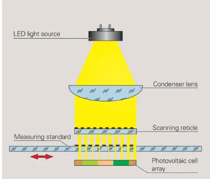
There are several approaches used to code the position using linear encoders. When

(24)

scanning is used[19]. A scanning reticle and a measuring standard scale are placed relative to

each other. The scanning reticle is made of transparent materials that parallel light can passes

through.

The incident light is modulated by the gaps of these two gratings when the measuring

standard is moving. When the gaps are aligned, light is not blocked and can be detected by

the photovoltaic cell array. The opposite case occurs when the gaps of one grating is blocked

by the line of the other, and no light can pass measuring standard. The illustration is shown in

Figure 2-8. On the occasions where the movement is relatively small or high resolution is

needed, another method called interferential scanning should be applied. A schematic view is

shown in Figure 2-9.

(25)

Figure 2-9 Interferential scanning method[19]

When the light passes through the scanning reticle, it is diffracted into three beams

with almost equal intensity with the order -1, 0,+1. These beams are diffracted again at the

scales of the measuring standard and reflected back to the scanning reticle where interference

occurs[19].

If relative motion occurs between the scanning reticle and the measuring standard,

there will be phase shifts for the light with order +1 and -1. If the grating moves by one

period, the shift of the “+1” light will be 2π in the positive direction while the shift of the “-1”

light is 2π in the negative direction. Thus, one period change of the grating causes a change

(26)

2-3 Summary

A review of four common optical encoders is presented in this chapter. The purpose

is to investigate the features of these encoders and point out their advantages and

disadvantages. This examination is to determine if they are suitable for the optical

positioning using an ordinary camera.

Each of these optical encoders has favorable properties of high accuracy, high

reliability and can code the position without direct contact [18,19]. However they are

relatively complex and can require attachment of precision machined encoding strips and

multiple detectors. They are also limited to measurement in one dimension and can’t freely

(27)

CHAPTER 3 Obtain the Reading of the Micrometer with a

Microscopic Camera

As an example of measuring linear motion we consider using a digital microscope

with and off-the-shelf micrometer. The micrometer is widely used for precise measurement

of small distance such as moving translation stages and optical components. The principle

idea is that by using a digital camera higher accuracy can be obtained rather than reading by

eye.

Figure 3-1 The experimental arrangement (left) and the camera used (right)[21]

The experimental arrangement is shown in Figure 3-1, and consists of a digital

microscope and bracer to hold the microscope a translation stage with a digital micrometer.

The camera is used to take pictures of the scales on the sleeve of the micrometer. The bracer

and clamp is used to hold the camera and adjust its position. The translation stage is

(28)

350 in this thesis[16]. When the thimble of the micrometer is being rotated, the translation

stage will move along the same direction. To check the accuracy of our method, the

micrometer is also equipped with a digital readout. This readout device uses a linear variable

differential transformer with a custom chip that contains calibration data to measure the

positions. The rated accuracy of the digital readout is 0.001 mm or 1 µm and are displayed on

a small LCD screen[16].

The reading on the LCD screen provides a reference that we compare with our

method. The important parameters of the micrometer in this thesis are shown below[16]:

1. Lead: 0.025 inch

2. Range: 1 inch

3. The number of the graduated markings on the thimble: 25, starting from ‘0’ to ‘24’.

4. The number of the major graduated markings on the sleeve: 11, starting from ‘0’ to

‘10’.

5. The number of the minor graduated markings on the sleeve: 20 above the axial line,

and 40 sub-divisions below the axial line.

From the above parameters, it’s clear that if the thimble is screwed out by one turn,

the axial movement of the micrometer will be 0.025 inch to the right. And the edge of the

thimble will move from the central line of one minor graduation to that of an adjacent minor

(29)

is screwed out by one division on the thimble. If the graduation on the thimble that coincides

with the axial line was graduation 0, then it would become graduation 1 after this operation.

The reading of the micrometer is determined by how many divisions and sub-divisions are

visible on the sleeve, and which graduation on the thimble coincides with the axial line or an

estimated position when there is no such a graduation:

R = S * 0.02495 + G*0.0010.

Where R is Reading, S is the number of complete sub-divisions that can be seen on

the sleeve and G is the estimated position on the thimble that coincides with the axial line.

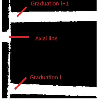
Figure 3-2 Example of experimental image

Thus in our experiments what we want to be able to do is accurately determine an

estimate for the graduation. If we know that value to high accuracy we will have an accurate

measurement of position. For example as shown in Figure 3-2, Graduation 0 and one

sub-division are visible on the sleeve, Graduation 10 on the thimble is seen to coincide with the

(30)

In general, the idea is to take a picture of the micrometer (Figure 3-3). Then digitize

the image to identify the positions of the rotating horizontal lines, and compare the position

of those lines with the horizontal reference line. Then using the knowledge of the spacing of

the marks on the micrometer determines the position accurately.

Figure 3-3 Obtaining the reading of a micrometer using a camera

This was accomplished in two steps. First using the LCD readout of the micrometer a

series of calibration images were taken for each turn of the thimble from graduation 0 to

graduation 24. This establishes a bijection of the axial line and horizontal lines on the thimble.

The program ran these 25 images as a batch file and then was used to form a table, where the

ration of the distance between the axial line and the horizontal lines corresponds to the linear

motion of the micrometer. This process is described in the section titled standard pictures.

(31)

expressed as a ratio. This can then be modified by a calibration factor using the series of

calibration images that have been obtained.

3-1 Obtaining standard pictures

A number of images focused on the ROI are taken using the platform shown in Figure

3-1. There are several requirements when taking the images:

1. The images should be taken in the same surroundings with almost the same light

source, the same shooting angle and the same distance from the lens;

2. The gray-scale of the images should be as even as possible. Avoid the situation that

some parts of the images are too dark or too bright;

3. The images should contain mainly the scales of the micrometer. And the ROI should

be made sure as clear as possible.

(32)

Figure 3-4 An example reference image of the ROI with a reading of 0.24995

3-2 Processing of the standard images

The processing includes crop, incline correction, threshold, removing noise and

converting the image from gray scale to black and white. As long as the images meet the

requirements stated above, a batch file can complete the processing quickly for many images

at a time. One example of the processed image is shown in Figure 3-4. Unnecessary part of

the image has been cropped out. These reference images are then stored for future use.

(33)

3-3 Calculation of the ratio

The special ratio refers to the ratio of the length of the last interval, which is not a

complete sub-division and the average length of the complete sub-divisions. The lengths are

obtained in pixels. (Figure 3-5)

Figure 3-6 A illustration of the sub-division and the varying interval

Continue taking Figure 3-4 as an example, a histogram of the distribution is shown in

Figure 3-6. The peaks have shown the locations of the linear graduations on the sleeve. The

thin small line shows the position of the edge of the thimble, which has overlapped with the

(34)

Figure 3-7 An intensity histogram of the reference image

The locations of the linear graduations are shown in Table 3-1. p is the position in

pixels.

Table 3-1 Locations of linear graduations of a reference image

NO. 1 2 3 4 5 6 7 8 9 10 11

p 52 117 183 247 313 377 443 508 573 638 706

Use the value of the position of one graduation to subtract that of the former one, the

lengths of the sub-divisions are obtained and shown in Table 3-2.

Table 3-2 Lengths of the sub-divisions of a reference image

NO. ₁ ₂ ₃ ₄ ₅ ₆ ₇ ₈ ₉ ₁₀

Length

(pixels) 65 66 64 66 64 66 65 65 65 68

The average length of the former 9 sub-divisions is 65.11. The reason why the last

(35)

and the thimble. Therefore, the position of the last graduation in this image is not reliable.

This problem is solved when images were taken for larger readings that the 11th graduation

can be distinguished. It is found that the position of the 11th graduation should be 705 by

comparison with other images. In this way the last graduation position are corrected for all

other similar situations.

As a result, the length of the varying interval is about 1 pixel in this image. The ratio

is defined as r,

The graduation on the thimble that coincides with the axial line is graduation 0. It is

desirable that the ratio is calibrated to 0.00%. Same procedures are done for other 23

reference images and a bijection of the ratio and graduation is obtained and shown in Table

(36)

Table 3-3 G and corresponding ratio of reference images Original length Original ratio Improved length Improved

ratio G

Ideal ratio''

1 1.53% 0 0.00% 0 0.00%

4 6.13% 3 4.59% 1 4.00%

6 9.19% 5 7.66% 2 8.00%

8 12.25% 7 10.72% 3 12.00%

11 16.85% 10 15.31% 4 16.00%

14 21.47% 13 19.94% 5 20.00%

15 22.94% 14 21.41% 6 24.00%

18 27.57% 17 26.03% 7 28.00%

21 32.21% 20 30.67% 8 32.00%

23 35.28% 22 33.74% 9 36.00%

27 41.41% 26 39.88% 10 40.00%

31 47.55% 30 46.01% 11 44.00%

33 50.69% 32 49.16% 12 48.00%

35 53.68% 34 52.15% 13 52.00%

38 58.37% 37 56.84% 14 56.00%

40 61.44% 39 59.91% 15 60.00%

43 65.95% 42 64.42% 16 64.00%

46 70.66% 45 69.12% 17 68.00%

48 73.62% 47 72.09% 18 72.00%

51 78.22% 50 76.69% 19 76.00%

54 82.95% 53 81.41% 20 80.00%

57 87.56% 56 86.02% 21 84.00%

60 92.17% 59 90.63% 22 88.00%

64 98.16% 63 96.63% 23 92.00%

(37)

The original length and original ratio stands for the interval length and the ratio that

obtained from the last step directly. And it’s not so accurate and useful as can be seen in the

last row of Table 3-4 that the ratio exceeds 100% when graduation 24 coincide with the axial

line. We assume that there is a system error and therefore a calibration is needed. The result

is the improved length and improved ratio. They are obtained by subtracting 1 pixel from the

original length. G is the number of the graduation that coincides with the axial line. The ideal

ratio is obtained by dividing G by 25.

The next step is to obtain the reading of an unknown experiment image by

interpolating its ratio r into Table 3-3.

One processed example image is shown as Figure 3-8.

Figure 3-8 A processed example image

The locations of the graduations and the length of the sub-divisions are obtained and

(38)

Table 3-4 The locations of the graduations and the length of the sub-divisions of the experimental image

NO. 1 2 3 4 5 6 7 8 9 10 11 11.X

p 96 169 244 317 392 465 541 614 689 762 840 *870

Length 73 75 73 75 73 76 73 75 73 78 **30 --

* The position of the edge of the thimble

** The length of the varying interval.

The average length of the sub-divisions is 74.4, and the improved ratio is roughly

By looking up Table 3-3, G of this image is found to be between 9 and 10. The

exactly position is calculated another way. The right part of the image is extracted and shown

as Figure 3-8.

(39)

i = 9 in Figure 3-8. As long as the exact position where the axial line coincides with

the edge of the thimble is obtained, the G for this image can be determined precisely.

Therefore, another intensity histogram is made and shown in Figure 3-9.

Figure 3-10 The histogram of the right part of the experiment image

The three peaks represent the positions of Graduation 9, the axial line and Graduation

10 respectively.

Table 3-5 Calculation of the precise location of the rotary graduations

Left edge position (pixel)

Right edge position (pixel)

Mean Value (pixel)

Graduation 9 13 44 28.5

Axial line 171 202 186.5

(40)

The ratio of the distance between Graduation 9 and Axial line and the distance

between Graduation 9 and Graduation 10, which is defined as , is found to be:

The final value of the reading is expected to be:

.

The reading on the LCD screen is . Take this reading as the

reference, the error is

.

It is in good agreement with the digital readout, and demonstrates the principle that

high accuracy can be obtained using image processing methods.

Potentially this type of measurement could be integrated into a small package and

(41)

CHAPTER 4 ANOTO DOT PATTERN TECHNOLOGY

4-1 Introduction of Anoto Dot Pattern Technology

Anoto Dot Pattern Technology was invented and developed by Anoto AB Group to

be used with their product digital pen for electronic paper applications. This technology can

establish an absolute position coordinate system to digitize paper by printing a special kind of

encoded dot pattern onto them.[13] Thus when one writes on a digital paper, the pen records

the coordinates which are then transferred to a computer.[14][15]

The Anoto system is highly developed and commercialized. The information

described about their technology is extracted from publicly available information on their

website and patents. They also have a software development kit, for third party developers to

use their pen. However we thought this only accesses information at a high level. In this

portion of the thesis we implement our own method of decoding the dot pattern to obtain the

coordinates, and then examine the possibility using this information to obtain precise

positioning information.

(42)

4-2 Principle of Anoto Dot Pattern Technology

This section summarizes the methods described by Anoto in their patents and is

meant to provide enough reference for the reader to understand the MATLAB code in

Appendix B.

The dot pattern, which has the form of a grid with a spacing of 0.3 mm, is made up of

lots of small black dots. The grid is called a raster in Anoto Patents[13,22] . The raster lines

are invisible both to human eye and optical reader. Instead of being located exactly at the

intersection of the raster lines (called the “nominal position”), each small dot is displaced

slightly near the intersection in one of the four directions: up, down, left and right. One

example of the four kinds of dot positions is shown in Figure 4-2 a~d.

(43)

Each kind of the dots, which is called position element, indicates a possible

combination of x and y coordinates. Therefore two bits of information are contained in each

element, one bit is used to encode a first dimension x, the other is used to encode a second

dimension y. An x-code, y-code pair is assigned to each of the four position elements, as

shown in Table 4-1.

Table 4-1 Conversion between Offset direction and code pair[13]

Offset direction x code y code

Left 1 0

Right 0 1

Up 0 0

Down 1 1

In this way, independent x and y codes can be read simultaneously if given a definite

piece of the dot pattern. One example is shown in Figure 4-3.

(44)

In order to identify a position, at least a piece of the dot pattern contains 6×6 dots is

needed[24]. But Anoto Dot Pattern utilizes an 8×8 array of dots[13], where the extra two

dots are introduced for rotation and error correction purposes. One of the most significant

properties that the pattern has is that an array formed by any 8×8 dots appears only once all

over the entire surface, which makes it possible to identify unique positions.

The reason why the pattern has the above property is that the code which it is encoded

into is designed using a special De Bruijn sequence[25,42,47]. This number sequence is

cyclic and the length of the sequence is intentionally designed to make any partial sequence

of a definite length taken from the main sequence occurs only once. In Anoto’s patents[13],

the special designed quasi De Bruijin sequence[25] is called the main number sequence

(MNS) and has a total of 63 numbers as follows:

0, 0, 0, 0, 0, 0, 1, 0, 0, 1, 1, 1, 1, 1, 0, 1, 0, 0, 1, 0, 0, 0, 0, 1, 1, 1, 0, 1, 1, 1, 0, 0, 1, 0, 1, 0,

1, 0, 0, 0, 1, 0, 1, 1, 0, 1, 1, 0, 0, 1, 1, 0, 1, 0, 1, 1, 1, 1, 0, 0, 0, 1, 1.

Any partial sequence of length 8 has a position value from 0 to 62. For example,

partial sequence ‘0, 0, 0, 0, 0, 0, 1, 0’ has the position value ‘0’, and ‘0, 0, 0, 0, 0, 1, 0, 0, 1’,

which is ‘0, 0, 0, 0, 0, 0, 1, 0’ shifted right by one, has the position value ‘1’.

The main number sequence is shifted up and down in columns and left and right in

rows by different numbers, and is repeated when it comes to its end. Therefore, the adjacent

two columns or two rows have a constant difference number. For example, as for the x

(45)

column k+1 contains the main number sequence shifted by m number of rows, the difference

number of these two columns will be (l-m) modulo 63. The difference numbers between

columns and rows form another important sequence called primary difference number

sequence (PDS). As can be easily observed, although each column and each row start with an

identical MNS shifted by different numbers, the PDS does not change from row to row for

the x direction, and from column to column for the y direction.

An 8×8 array of this kind of dot pattern has eight columns and eight rows which can

be encoded into eight vertical partial sequences and eight horizontal partial sequences with

each partial sequences has the length of eight. Each partial sequence then has a

corresponding position number for x direction and y direction separately. Besides, two partial

PDS of length 7 for the x and y directions can also be obtained separately.

(46)

What position the partial PDS is in the whole PDS is one of the key pieces of

information that tells us about the coordinates. Although the difference numbers are obtained

by the differences modulo 63 and are therefore all between 0 and 62, only those with values

between 5 and 58, that is 54 = 2*33 numbers are usable. If a difference number is found out

of [5, 58], then an error must have occurred.

In practice, the primary difference sequence is further converted into so-called

secondary difference number sequences (SDS) for calculation and detection and

error-correction reasons[17]. For any difference number d belongs to [5, 58], a bijection can be

established using rules described below, where a1, a2 and a4 have the values from 0 to 2 and

a3 has the values from 0 to 1.

;

For example, if d = 35, then d = 5 + 0 + 3 + 9 + 18 = 5 + 0 + 1*3 + 1*32 +1*2*32. So

d =35 convert to (a1, a2, a3, a4) is (0, 1, 1, 1). In this way, the primary difference sequence is

converted to four secondary difference sequences, as shown in Table 4-5.

(47)

If the position numbers of the partial secondary difference sequences in the whole

secondary difference sequences are found, then the position number of the partial PDS can be

calculated using Chinese Remainder Theorem[44]. Therefore, four secondary difference

number sequences A1~A4 are introduced as below[13].

A1=[0,0,0,0,0,1,0,0,0,0,2,0,1,0,0,1,0,1,0,0,2,0,0,0,1,1,0,0,0,1,2,0,0,1,0,2,0,0,2,0,2,0,1,1,0,

1,0,1,1,0,2,0,1,2,0,1,0,1,2,0,2,1,0,0,1,1,1,0,1,1,1,1,0,2,1,0,1,0,2,1,1,0,0,1,2,1,0,1,1,2,0,0,0,

2,1,0,2,0,2,1,1,1,0,0,2,1,2,0,1,1,1,2,0,2,0,0,1,1,2,1,0,0,0,2,2,0,1,0,2,2,0,0,1,2,2,0,2,02,2,1,

0,1,2,1,2,1,0,2,1,2,1,1,0,2,2,1,2,1,2,0,2,2,0,2,2,2,0,1,1,2,2,1,1,0,1,2,2,2,2,1,2,0,0,2,2,1,1,2,

1,2,2,1,0,2,2,2,2,2,0,2,1,2,2,2,1,1,1,2,1,1,2,0,1,2,2,1,2,2,0,1,2,1,1,1,1,2,2,2,0,0,2,1,1,2,2]

A2=

[0,0,0,0,0,1,0,0,0,0,2,0,1,0,0,1,0,1,0,1,1,0,0,0,1,1,1,1,0,0,1,1,0,1,0,0,2,0,0,0,1,2,0,1,0,1,2,

1,0,0,0,2,1,1,1,0,1,1,1,0,2,1,0,0,1,2,1,2,1,0,1,0,2,0,1,1,0,2,0,0,1,0,2,1,2,0,0,0,2,2,0,0,1,1,2,

0,2,0,0,2,2,2,1,0,1,2,2,0,0,2,1,2,2,1,1,1,1,1,2,0,0,1,2,2,1,2,0,1,1,1,2,1,1,2,0,1,2,1,1,1,2,2,0,

2,2,0,1,1,2,2,2,2,1,2,1,2,2,0,1,2,2,2,0,2,0,2,1,1,2,2,1,0,2,2,0,2,1,0,2,1,1,0,2,2,2,2,0,1,0,2,2,

1,2,2,2,1,1,2,1,2,0,2,2,2]

A3=[0,0,0,0,0,1,0,0,1,1,0,0,0,1,1,1,1,0,0,1,0,1,0,1,1,0,1,1,1,0,1]

A4=[0,0,0,0,0,1,0,2,0,0,0,0,2,0,0,2,0,1,0,0,0,1,1,2,0,0,0,1,2,0,0,2,1,0,0,0,2,1,1,2,0,1,0,1,0,

(48)

0,2,2,0,1,0,2,1,0,1,2,1,1,0,1,1,1,2,2,0,0,1,0,1,2,2,2,0,0,2,2,2,0,1,2,1,2,0,2,0,0,1,2,2,0,1,1,2,

1,0,2,1,1,0,2,0,2,1,2,0,0,1,1,0,2,1,2,1,0,1,0,2,2,0,2,1,0,2,2,1,1,1,2,0,2,1,1,1,0,2,2,2,2,0,2,0,

2,2,1,2,1,1,1,1,2,1,2,1,2,2,2,1,0,0,2,1,2,2,1,0,1,1,2,2,1,1,2,1,2,2,2,2,1,2,0,1,2,2,1,2,2,0,2,2,

2,1,1]

They have a length of 236, 233, 31 and 241 respectively. The lengths are chosen

relatively prime to each other so that the lowest common multiple of the four sequences will

be the product of their lengths. Then the respective places p1, p2, p3 and p4 of the partial

sequence of length 5 in these four secondary difference sequences can be determined using

the same method of determining the place P of the partial sequence in the primary difference

sequence, which has been stated above. And they have a relation listed below:

P ≡ p1 (mod l1)

P ≡ p2 (mod l2)

P ≡ p3 (mod l3)

P ≡ p4 (mod l4)

Where l1, l2, l3, l4 are the lengths of the secondary difference sequences that have

values 236, 233, 31, 241 respectively in Anoto’s application. As a result, P can be calculated

using Chinese Remainder Theorem[26].In fact, there is no need to calculate the position

number P of the partial PDS, since we know the four position numbers p1, p2, p3, p4 of the

(49)

between (p1x, p2x, p3x, p4x) and x, and (p1y, p2y, p3y, p4y) and y, where x, y is the

coordinates in x and y directions. Here x stands for the xth column, y stands for the yth row,

which gives us the information directly. This is exactly what we utilize in this thesis.

Another factor that is important in Anoto positioning is called the “Section”[13]

. Since

there are 63 different place numbers for the primary difference sequence, there are 63

possible values which can start the very first x coordinate and first y coordinate respectively.

That is in total 63*63 = 3969 different “versions” of the dot pattern[13]. And which two

numbers starts the first column and first row are called section number for the x direction and

section number for the y direction respectively. This is useful when manage numerous pieces

of surface with a huge number of area in sum. Since the surface used in this thesis is far

smaller, there is no problem of managing different ‘sections’ of the surface. Therefore it is

unnecessary to calculate the section number. Actually, they are provided as a known

(50)

CHAPTER 5 DESIGN OF AN OPTICAL POSITIONING

SYSTEM

The design of the optical positioning system consists of the design of a hardware

system and a software system. The hardware system contains four devices as shown in

Figure 5-1: (a) a translation stage with a micrometer; (b) a Dino Microtouch Camera with an

USB connector[21]; (c) a camera bracer; (d) a pedestal.

Figure 5-1 The hardware of the optical positioning system

The software system is a program developed using Matlab scripts to process images

and make calculations. The entire process of the experiment is schematically shown in the

(51)

Figure 5-2 Flowchart of the experiment

The Anoto Dot Pattern that we use in this thesis comes from a test paper of their

products. We used a Canon Laser jet printer with a high resolution of 1200 dpi to print the

dot pattern on to several pieces ordinary paper.

5-1 Image Preparation

An enlarged partial image of the paper with printed dot patterns is shown in Figure 5-3.

(52)

The number of dots contained in the array in Figure 5-2 is the minimum for enough

information to identify a position when it is being decoded. But a typical image taken by the

camera could have much more dots as shown in Figure 5-4. Those black curves are written

pen strokes. It can be seen that grid spacing of the dot pattern is a little smaller than the width

of the pen strokes and the raster lines are not actually printed on the paper.

Figure 5-4 A typical image taken by the camera at 60X magnification

5-2 Preprocessing

After the image is taken, the next step is to preprocess it to prepare it for decoding

process. The preprocessing section consists of conversion into gray-scale image, thresholding,

removing noise and converting to a black and white image. These processes can be done

manually to get the best image quality for decoding with a relatively large time cost and

human-attention, or automatically using a series of batch scripts with a much smaller time

(53)

determined by the printing quality of the original image. One set of the Figures showing

(54)

(55)

5-3 Decoding

The image shown as Figure 5-6 (e) is ready for decoding. Firstly, Each blob in the

preprocessed image is identified using Matlab scripts[27,28]. Then the blobs will be replaced

with their own centroids, or the center of gravity. The coordinates of these centroids are

obtained in pixels. Using these coordinates, a new image containing dots of only one pixel is

obtained as shown in Figure 5-6 (a).

(a) (b)

Figure 5-6 An example image of one-pixel dots and its FFT

Figure 5-6 (b) is a binary image of the Fast Fourier Transform of Figure 5-6 (a). It is

thresholded to filter out unnecessary information but the small grid which is made up of nine

dots in the middle. The relative position of the nine dots tells us if a rotation correction is

needed for the original image[29].This step is essential to make sure the decoding process

(56)

the 9-dot grid will look like a parallelogram other than a rectangular. The value of the angle

used to correct the rotation can be calculated by using the slopes of the sides of the

parallelogram. Then the original image could be rotated back to balance the tilt.

Next, the centroids of the blobs in the image are divided into columns and rows. If

there are M×N blobs in the image, the coordinates of the centroids are recorded into two

M×N matrices, one for the x-coordinates and the other for the y-coordinates.

As for the x-coordinates, from the relative positions inside a same column, the dots

could be divided into 3 kinds: left (L), medium (M), and right (R), depending on which

direction the dot is offset in x dimension. If the number of dots is relatively large, there is a

big chance that all three kinds of the dots can be found in a single column. But if the number

of dots is relatively small, for example only 6~10 dots per column, there is a good chance

that only two kinds of the dots (L and M, or M and R) can be found in a column. Sometimes

extreme situation happens that only one kind of the dots is found in a single column.

Fortunately, the three situations can be easily identified by comparing the width of each

column to the mean value of themselves.

In our embodiment, if the width of the column is larger than 2/3 of the mean value,

we know the column contains all three kinds of dots. If the width is smaller than 1/3 of the

mean value, then the column has probably only one kind of dots. And if the width of the

column is between 1/3 and 2/3 of the mean value, then the column should have 2 kinds of

(57)

It is easy to find out in which direction the dots are offset for the first kind of column.

Since all we need to do is further divide the dots in the column into three kinds. The smallest

1/3 is the left ones, the medium 1/3 the medium ones, the largest 1/3 the right ones.

Things get more complicate when it comes to the latter two kinds of columns. The

solution we give is to take the other coordinates into account based on the property that

Anoto Dot Pattern has. We know that there are in total four directions the dots can be

displaced in, two in x dimension, the other two in y dimension. And we assign a direction

indicator as list in the table below:

Table 5-1 Conversion between offset direction and offset indicators

Offset direction Indicator in x dimension

Indicator in y dimension

Left -1 0

Right 1 0

Up 0 1

Down 0 -1

As can be seen in Table 5-1, one of the two indicators must be 0, but they cannot be 0

simultaneously. This property is useful that once we cannot determine the offset direction of

the dot in one dimension, we can search in another dimension. Usually the problem will be

solved.

Once the offset direction of each dot is determined, it is important to make sure it’s

correct. Since the quality of the printing or image can be low and the image can be distorted.

(58)

After the error-correction section, we can decode the dot patterns into codes both in x

and y direction as shown in Table 4-1. And then we can utilize the x codes and y codes,

following the directions stated in Chapter 4 to determine the coordinates of columns and

rows. An example of the process is given below. A preprocessed binary image is shown in

Figure 5-7.

Figure 5-7 A preprocessed image ready for decoding (60X)

The first thing we need to do is to check if the dot pattern contained in this image is

inclined. If it is not, then the virtual raster lines should be parallel to the coordinate axis. And

this is what we desire. Otherwise, we must find out how much it is inclined and rotate the

image to the opposite direction to cancel the effect. Of course, sometimes it is not easy to

judge whether the image is inclined and needs rotation-correction by human eye, since the

(59)

the Fast Fourier Transform of the image and solve this problem in Frequency Domain. The

FFT of Figure 5-7 is shown in Figure 5-8 (a) below.

Before the use is made of it, a threshold is made to filter out unnecessary information.

This process needs to be done manually to make sure all the information, except the nine dots

in the middle of the image, is filtered. These nine dots form a small parallelogram. The angle

made by the sides of the parallelogram and the horizontal and vertical directions tells if the

virtual raster lines are parallel to the coordinate axis.

Figure 5-8 Using FFT of the one-pixel dots image to correct the incline

Since the 9-dot parallelogram is made up of 4 smaller parallelograms, we can look

into the smaller parallelograms for simplicity. According to the geometry relations of these

dots, the calculations are made as follows:

(60)

2. Find the four nearest dots to the center dot in all the quadrants. It is done by

searching the dot that has the smallest Euclidean distance to the center dot in all the four

quadrants. And they are P1(257.33, 269.33), P2(244.67, 257.33), P3(256.67, 244.67) and

P4(269.33, 256.67).

3. Determine the four slopes of the straight lines P1Pc, P2Pc, P3Pc and P4Pc. The result is

shown in Table 4-2

Table 5-2 Calculation of the incline angle

P1Pc P2Pc P3Pc P4Pc

Slope 0.9996 0.0270 0.9996 0.0270

Angle 88.45º 1.55º 88.45º 1.55º

Analyze the angles in Table 5-2, and it is found that the dot pattern is 1.55 degree

inclined. Rotate the original image -1.55 degree to for rotation-correction. The corrected

image is shown as Figure 5-9.

(61)

Then the x, y coordinates of the centroids are obtained and shown in the Table 5-3:

Table 5-3 x, y coordinates (in pixels) of the centroids (a) the x coordinates (b) the y coordinates

(a) the x coordinates

(b) the y coordinates

Use the first column as an example. The minimum value of x coordinates is 19.5740,

and the maximum value of x coordinates is 33.0250. Thus the difference of these two is ∆1 =

33.0250-19.5740 = 13.4510. We can calculate the difference of maximum and minimum for

every column. The result is shown in Table 5-4.

Table 5-4 Differences of maximum and minimum of each column

Column ∆1 ∆2 ∆3 ∆4 ∆5 ∆6 ∆7 ∆8

(62)

Therefore, the maximum difference is 15.5719.

1/3 of the maximum difference: 5.1906

2/3 of the maximum difference: 10.3813

The columns that have a difference larger than 10.3813 (Column Class A): Column 1,

Column 2, Column 3, Column 4 and Column 6

The columns that have a difference between 5.1906 and 10.3813 (Column Class B):

Column 5, Column 7 and Column8.

As for the Columns in Class A, there are three kinds of dots (considering only in x

direction, so the dots that offset upwards and downwards count as one ‘medium’ kind).

Again, take the first Column as an example, divide the spacing between the dot with the

minimum x coordinate and the dot with the maximum x coordinate into three intervals of

equal length in x direction: [19.5740, 24.0577), [24.0577, 28.5414) and [ 28.5414, 33.0250] .

Assign offset indicator ‘-1’ to the dots whose x coordinate falls in the first interval (left ones),

‘0’ to the dots whose x coordinate falls in the second interval (medium ones), and ‘1’ to the

dots whose x coordinate falls in the last interval.

As for the Columns in Class B, there are only two possible combinations of offset

directions for the dots--the left ones and the medium ones, or the medium ones and the right

ones. In this situation, we can first divide the spacing between the dot with the minimum x

coordinate and the dot with the maximum x coordinate into two intervals of equal length.

(63)

[196.1010, 200.9216]. Assign offset indicator ‘-2’ to the dots whose x coordinate falls in the

first interval and offset indicator ‘2’ to the dots whose x coordinate falls in the second

interval. And the offset direction indicators are then obtained and shown in Table 5-5.

Table 5-5 Unmatched Offset direction indicators in x, y directions (a) in the x direction and (b) in the y direction

(a) in the x direction

(b) in the y direction

The offset indicator ‘-2’and ‘2’ are only temporary. They do not tell the actual offset

direction of the dots, but just indicate the position relation inside a column. In order to find

out the actual offset direction, we need to account for the offset indicator in y direction,

which has been shown in Table 5- 5 (b). It can be easily found that the common feature of the

(64)

Now focus on the offset indicator of column 2 in y direction. They are -1, 2, -1, 1, -1,

1, 2, 0. Together with those in x direction, they are made into pairs as (-2,-1), (-2,2), (-2,-1),

(-2,1), (-2, -1), (-2,1), (-2, 2), (2,0). We know that the offset indicators in x and y direction

should not be 0 simultaneously, but at least one of them must be 0. Thus, the factor pairs are

improved to (0,-1), (-2, 2), (0,-1), (0,1), (0,-1), (0,1), (-2, 2), (2, 0). Then we get an inference

that in the second column, the offset indicator ‘-2’ is actually ‘0’, and therefore the offset

indicator ‘2’ should be ‘1’.

Besides, notice that the last pair is (2,0), Because ‘2’ indicates that the dot is in the

relatively right half of the dots distribution and its counterpart in y direction is already ‘0’, it

must be ‘1’. This is consistent with the above inference. Finally, the offset indicator for the

fifth column in x direction should be: 0, 0, 0, 0, 0, 0, 0, 1. Similar process are done for the

other two columns. The updated results of all the columns are shown in Table 5-6 (a). The

process for the y direction is similar and the results are shown in Table 5- 6(b). The whole

(65)

Table 5-6 Offset direction indicators after first correction (a) in the x direction and (b) in the y direction

(a) in the x direction

(b) in y direction

However, the offset indicators are not finally verified. As can be seen in Table 5-6(a)

and (b), the indicator pairs at {1,1},{3,3} and {1,8} are (-1,1), (-1,1) and (0, 0) respectively

({L,M} means the Lth row and the Mth column). These indicator pairs cannot create correct

x-code and y-x-code. The solution in this thesis is to reconstruct the virtual raster lines[23].

Once the offset indicators are obtained for both x and y directions, it becomes easy to

(66)

Figure 5-10 The dot pattern with reconstructed visible raster lines

Since the raster lines are obtained through the positions of the dots, which may have

been distorted during processing, the raster lines may not equally spaced. However, with the

aid of the raster lines, the offset directions of each dot become even clear. And this is a

complementary method to make sure offset indicator is correctly obtained. Take the indicator

pair at {1,1} for example.

The distance between the dot and the raster line in the x direction:

Dx = 23.8882 - 25.7418 = -1.8536;

The distance between the dot and the raster line in the y direction:

(67)

And for the absolute value, abs(Dy) >abs(Dx).

Thus the offset direction is determined to be in the y direction. The indicator is

assigned ‘1’ with the sign determined by the sign of Dy. Therefore, the indicator pairs at {1,1}

has been corrected from (-1,1) to (0,1).

Table 5-7 Final offset direction indicators (a) in the x direction and (b) in the y direction

(a) in the x direction

(b)in the y direction

The x, y codes then are obtained by converting the indicator pairs through the

(68)

Table 5-8 Corresponding x, y codes

Then we can decode in two dimensions respectively.

For the x direction, from Table 5-5(a), six vertical partial sequences are obtained as

follows: 00110101, 01001000, 10011010, 10010000, 10101000, 10000111, 10100100 and

10001110. The corresponding places of these partial sequences in the main number

sequences are

47, 14, 46, 15, 32, 18, 13, 57.

The primary difference sequence is further obtained as

30, 32, 32, 17, 49, 58, 44.

(69)

Table 5-9 An example of converting primary difference number sequence into secondary difference number sequences

d 30 32 32 17 49 58 44

a1 1 0 0 0 2 2 0

a2 2 0 0 1 2 2 1

a3 0 1 1 1 0 1 0

a4 1 1 1 0 2 2 2

The four partial sequences of length 5 are ‘10002’ for A1, ‘20012’ for A2,

‘01110 ’for A3, ‘11102’ for A4. The corresponding place numbers are listed below:

p1 = 119

p2 = 147

p3 = 25

p4 = 178

As long as the section number in x direction is known, or the four such numbers for

the first 8×8 array of the dot pattern are obtained, we can assign a column coordinate.

For the first 8×8 array, p1 to p4 are obtained as

p1= 32

p2= 57

p3= 12

(70)

Since the p1 to p4 get larger by one consecutively when the region of interest is

moved one column right, an infinite table can be established like below:

Table 5-10 The relation between column number and the four place numbers

Column 1 Column 2 Column 3 … Column x …

p1 32 33 34 … 119 …

p2 57 58 59 … 147 …

p3 12 13 14 … 25 …

p4 96 97 98 … 178 …

The ranges of p1, p2, p3 and p4 are 0 to 235, 0 to 232, 0 to 30 and 0 to 240

respectively. Identical combinations of p1, p2, p3 and p4 occur every l1×l2×l3×l4 = 236×

233×31×241 = 410815348 columns. That is 410815348×0.3 mm = 123244604.4 mm

=123.2 km, which is much larger than the dimension of test papers used in this thesis.

By looking up the Table 5-10, which is established using Matlab, the column

corresponding to (119, 147, 25, 178) is found to be column 324, which means that the first

column of the 8×8 array is column 324 of the whole surface. So the last column of the 8×8

array is column 331.

A similar process is made for the y direction. Instead of using vertical partial

sequences in Table 5-5, horizontal partial sequences are used. They are 00001110, 1000001,

(71)

secondary difference sequences are (50, 87, 11, 207). And the place numbers for the first row

of the dot pattern are (224, 19, 4, 155), then a similar table to Table 5-10 is obtained for the y

direction, shown as Table 5-11.

Table 5-11 The relation between row number and the four place numbers

p1 p2 p3 p4

Row 1 224 19 4 155

Row 2 225 20 5 156

Row 3 226 21 6 157

… … … … …

Row y 50 87 11 207

… … … … …

By looking up the Table 5-11, the row coordinate corresponding to (50, 87, 11, 207)

is Row 535. Thus the rows that are included in the 8×8 array of interest are Row 535 to Row

542. The decoding is complete and successful.

5-4 Calculate the movement distance

With any 6×6 array or 8×8 array of the dot pattern being successfully decoded, we

can quickly get the accurate position information of the object that we’re interested in on the

digitized surface just by taking pictures of the region of interest[30,31]. If we record the

position information of an object at a first position and that of the object at a second position,

(72)

As an example we can consider the case of when the position information of the

background dot array is known. This is shown in Figure 5-11. This can be a little impractical

since it assumes that the image is taken before and after the object is on the page, but it

shows in principle how the method can be used. However, in the case of a pen where the dots

are reflective in the infrared, and the ink from the pen is transparent to the infrared, this

method should work. In both cases- as an extension of this- is if the field of view is wide

enough and as long as one 8×8 can be used to obtain the absolute coordinate position, that

information can be used to extrapolate information about the occluded dots. This information

can be used to subtract dots from the image.

(a) (b) (c)

Figure 5-11 (a) the preprocessed image of the region of interest, with the object (the circle) at its starting position (b) the known dot pattern of the background, which will provide the position of the region (c) extracted from (a), which is a binary image of the