An Innovative Approach to optimum solution of a Transportation Problem

(1)

ISSN(Online) : 2319-8753 ISSN (Print) : 2347-6710

International Journal of Innovative Research in Science,

Engineering and Technology

(An ISO 3297: 2007 Certified Organization)

Vol. 5, Issue 4, April 2016

An Innovative Approach to optimum solution

of a Transportation Problem

Prof. Reena. G. Patel1 , Dr. P.H.Bhathawala2

Assistant Professor, Department of Applied Science and Humanities S.P.C.E, Visnagar, North Gujarat, India1 Professor and Head (Retired) Veer Narmad South Gujarat University, Surat, India2

ABSTRACT: Transportation problem isa one of the most tools which is widely used n the field of operation

Research and other fields like Engineering, business management. In this paper, we are trying to find the optimum solution of a transportation problem using the method named “An Innovative Approach to optimum solution of a Transportation Problem.” We are presenting the algorithm for the above method, which gives the initial Basic Feasible Solution as well as either optimum solution or near to optimum solution. The illustrations herewith make the simplicity to understand the above algorithm. Also it can be assume that the proposed algorithm gives an optimal solution nearly comparable to Modi’s method in less time of period.

KEY WORDS: Transportation, Optimality, Basic feasible solution, linear programming, optimal solution.

I. INTRODUCTION

Transportation problem is oldest approach in Optimization. The usual characteristics are since 1940’s and later. Tolsto (1930) was a base in operations research and hence a published a book on transportation planning by the National commissariat of Transportation of Soviet union, The article is named as methods of ending the minimal total kilometrage in cargo- transportation problem and proved a number of solutions, approaches including the famous idea that an optimum solution does not have any negative cost cycle in its residual graph. Though he was not able to prove, the fact that checking the cycle condition is sufficient for optimality.Transportation problem play an important role in logostics and supply chain management foe reducing the cost and improving the service. There are different algorithms have been developed for solving the transportation problem when the cost coefficients and the supply and demand quantities are known exactly. In many practical situations, the supply and demand quantities in transportation problems are hard enough because of some change in economic conditions. It was first studied by F.L.Hitchcock in1941, then by T.C.Koopmans in 1947.And finally put it in a frame work of linear programming and solved by simplex method by G.B.Dantzig IN1951.The Simplex method is not suitable for the Transportation problem especially for large scale transportation problem due to its special structure of model in 1954 charnes and cooper was developed Stepping Stone method.

Sudhaker etal proposed Zero Suffix method for finding an optimal solution for Transportation problem directly in 2012. This paper presents a new simple approach to solve the transportation problem. Hence the proposed method helps to get directly optimal solution with less iterations and its generacy. The algorithm of the approach is detailed in the paper and finally numerical examples are given to illustrate the approach the minimized cost comparison table is given.

II. MATHEMATICAL MATERIALS AND OTHER ASPECTS

(2)

International Journal of Innovative Research in Science,

Engineering and Technology

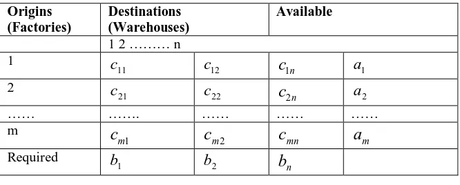
transportation model, suppose that m factories supply certain items to n warehouses. As well as, let factory(i=1,2,……,m) produces

a

_iunits, and the warehouses j(j=1,2,….,n) requires

b

_j

Units. Furthermore, suppose the cost of transportation from factory i to warehouse j is

c

_ij.The decision variables

x

_ijis being the transported amount from the factory i to the warehouse j. typically, our objective is to find the transportation pattern that will minimize the total of the transportation cost (see table 1).

Table 1: The model of a transportation problem

There are two types of Transportation Problem namely

(1) Balanced Transportation Problem and (2) Unbalanced Transportation Problem.

Definition of Balanced Transportation Problem: A Transportation Problem is said to be balanced transportation problem if total number of supply is same as total number of demand.

Definition of Unbalanced Transportation Problem: A Transportation Problem is said to be unbalanced transportation problem if total number of supply is not same as total number of demand.

Basic Feasible Solution:

Any solution Xij  0 is said to be a feasible solution of a transportation problem if it satisfies the constraints. The feasible solution is said to be basic feasible solution if the number of nonnegative allocations is equal to (m+n-1) while satisfying all rim requirements, i.e., it must satisfy requirement and availability constraint. There are three ways to get basic feasible solution.

1) North West Corner Rule

2) Minimum Cost Method or Matrix Minima Method 3) Vogel’s Approximation Method or Regret Method 4) Genetic Algorithm

5) Row minimum method 6) Column minimum method

Optimal Solution: A feasible solution of transportation problem is said to be optimal if it minimizes the total cost of transportation. There always exists an optimal solution to a balanced transportation problem .We start with initial basic feasible solution to reach optimal solution which is obtained from above three methods. We then check whether the number of allocated cells is exactly equal to (m+n-1), where m and n are number of rows and columns respectively. It works on the assumption that if the initial basic feasible solution is not basic, then there exists a loop. Here, we explain the MODI’S method to attain the optimality.

Origins (Factories)

Destinations (Warehouses)

Available

1 2 ……… n 1

11

c

₁₂

c

₁_n

a

1

2

21

c

22

c

₂_n

a

2

…… ……. …… …… …… m

1

m

c

_m₂

c

_mn

a

_m

Required

1

(3)

International Journal of Innovative Research in Science,

Engineering and Technology

III. ALGORITHM OF MODIFIED DISTRIBUTION (MODI) METHOD

Step: 1 For an initial basic feasible solution with (m+n-1) occupied (basic) cells, calculate ui and vj values for rows and columns respectively using the relationship Cij = ui + vj for all allocated cells only. To start with assume any one of the ui or vj to be zero.

Step :2 For the unoccupied (non-basic) cells, calculate the cell evaluations or the net evaluations as

Δij = Cij – (ui + vj).

Step: 3

a) If all Δij > 0, the current solution is optimal and unique.

b) If any Δij = 0, the current solution is optimal, but an alternate solution exists.

c) If any Δij < 0, then an improved solution can be obtained; by converting one of the basic cells to a non basic cells

and one of the non basic cells to a basic cell. Go to step IV.

Step: 4 Select the cell corresponding to most negative cell evaluation. This cell is called the entering cell. Identify a closed path or a loop which starts and ends at the entering cell and connects some basic cells at every corner. It may be noted that right angle turns in this path are permitted.

Step:5 Put a + sign in the entering cell and mark the remaining corners of the loop alternately with – and + signs, with a plus sign at the cell being evaluated. .Determine the maximum number of units that should be shipped to this unoccupied cell. The smallest one with a negative position on the closed path indicates the number of units that can be shipped to the entering cell. This quantity is added to all the cells on the path marked with plus sign and subtract from those cells mark with minus sign. In this way the unoccupied cell under consideration becomes an occupied cell making one of the occupied cells as unoccupied cell. Repeat the whole procedure until an optimum solution is attained i.e. Δij

is positive or zero. Finally calculate new transportation cost.

Algorithm for Proposed Method:

Step:1 Construct the Transportation matrix from the given transportation problem.

Step:2 Find the smallest cost from each row and subtract the smallest cost from each element of the row.

Step:3 Find smallest cost from each column and subtract the smallest cost from each element of the column.

Step: 4Compare the minimum of supply or demand whichever is minimum then allocate the min(supply or demand )at the place of minimum value of related row or column.

If tie at the place of minimum value in supply or demand then allocate at the maximum of supply or demand is observed.

Step: 5 After performing step-4, delete the row or column for further allocation where supply from a given source is depleted or the demand for a given destination is satisfied.

Step: 6 Repeat step-4 and step-5 unless and until all the demands are satisfied and all the supplies are exhausted.

Step:7 Now total minimum cost is calculated as sum of the product of cost and corresponding allocated Value of supply/demand.

i.e Total cost= _ij

n

i n

j ij

x

C

 

1 1

Numerical Examples (Proposed Method):

(4)

International Journal of Innovative Research in Science,

Engineering and Technology

By applying the proposed method, allocations are obtained as follows,

The total cost from these allocations is 1200 units.

2). Consider the following cost minimizing transportation problem

Supply

13 18 30 8 8 55 20 25 40 10 30 6 50 10 11

Demand 4 7 6 12 Total=29

By applying the proposed Method, Allocations are obtained as follows,

Supply

4

13 18 30

4 8

8

55

4 20

6 25 40

10

30

3 6 50

8 10

11

Demand 4 7 6 12 Total=29

1

D

2

D

₃ Supply

1

S

11 9 6 40

2

S

12 14 12 50

3

S

10 8 10 40

Demand 55 45 30 Total=130

1

D

₂

D

₃ Supply

1

S

11 10

9

30 6

40

2

S

15

12

14 12 50

3

S

5

10

35 8

10 40

(5)

International Journal of Innovative Research in Science,

Engineering and Technology

The Total cost from these allocations is 412 units.

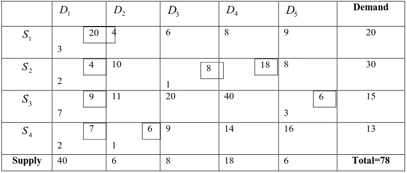
3) Consider the following cost minimizing transportation problem

1

D

2

D

3

D

4

D

5 Demand

1

S

3 4 6 8 9 20

2

S

2 10 1 5 8 30

3

S

7 11 20 40 3 15

4

S

2 1 9 14 16 13

Supply 40 6 8 18 6 Total=78

By applying the proposed Method, Allocations are obtained as follows,

1

D

2

D

3

D

4

D

5 Demand

1

S

20

3

4 6 8 9 20

2

S

4

2

10 ₈ 1

18 8 30

3

S

9

7

11 20 40 6 3

15

4

S

7

2

6 1

9 14 16 13

Supply 40 6 8 18 6 Total=78

The Total cost from these allocations is 267 units.

Comparison:

Comparison of total cost of Transportation problem of above examples between MODI method and proposed method is:

Table No: Problem Dimension

MODI’S Method

Proposed Method

1 3×3

1200

2 3×4

412

(6)

International Journal of Innovative Research in Science,

Engineering and Technology

IV. CONCLUSION

In this paper, we have developed the algorithm is very helpful as having less computations and also required the short time of period for getting the optimal solution.

Also in this paper we have described the comparison between the MODI’s method and the proposed method and also the solution is nearly same according to the MODI’s method.

From this method we are getting an optimal solution without solving the Initial Basic Feasible solution. Thus the proposed method provide an optimal solution nearly to the MODI”s Method.

REFERENCES

1. Arsham H and Khan AB (1989). A Simplex- type ,algorithm for general transportation problems; An alternative to stepping-stone. Journal of Operational Research Society 40(6) 581-590.

2. Charnes, Cooper (1954). The Stepping-Stone method for explaining linear programming. Calculation in transportation problems. Management Science 1(1)49-69.

3. Dantzig GB (1963). Linear Programming and Extensions, New Jersey:Princeton University press. Goyal SK (1984). Improving VAM for unbalanced transportation problem, Journal of Operational Research Society 35(12) 1113-1114.

4. Gass S (1964). Linear Programming Mc-Graw-Hill New York.

5. Garvin WW (1960). Introduction to Linear Programming, Mc-.Graw-hill New York.

6. Hitchcock FL (1941). The distribution of a product from several sources to Numerous localities, Journal Of Mathematical Physics 20 1941 224-230.

7. Kirca and Statir (1990). A heuristic for obtaining an initial solution for the transportation problem, Journal of operational Research Society 41(9) 865-867.

8.Koopmans TC (1947). Optimum Utilization of the Transportation system proceeding of the international stasttical conference, Washington D.C.

9. Ping Ji,Chu KF (2002). A dual-Matrix approach to the transportation problem. Asia- Pacific Journal of Operation Research 19(1) 35-45.

10. Reinfeld NV ,Vogel WR (1958 )., Mathematical Programming New Jersey Prentice- Hall, Englewood Cliffs.

11. Shore HH ( 1970). The Transportation Problem and the Vogel Approximation Method, Decision Sciences 1(3-4) 441-457.