Multiconductor signal propagation in distribution line carrier networks

John Dongbin Suh

Center for Communications and Signal Processing Department of Computer Science

North Carolina State University

CCSP-TR-88/11~

Suh, John D. Multiconductor Signal Propagation in Distribution Line

Carrier Networks (under the direction of J.B. O'Neal, Jr.)

A mathematical model for predicting multiconductor signal

propagation in distribution line carrier networks is formulated and

tested with empirical data. The multiconductor model accounts for

general source and load termination conditions and can be extended for

analyses of multiconductor systems of order 'n'. Current and voltage

propagation measurements (a total of 14 sets) conducted on actual

three-phase distribution lines are presented. It is shown that

certain discontinuities set up different wave patterns on each line,

which introduce electromagnetic coupling effects between phase

conductors at carrier frequencies.

Several test cases are computer-simulated to assess the

validity of the mathematical model. It is found that, overall, the

predicted results based on the multiconductor model agree with that

of the measured data, and hence, the mathematical model is valid.

The derivation of the distributed parameters of the multiconductor

model is presented and implemented in a computer simulation. It

is concluded that although the theoretically derived parameters are

adequate in predicting signal profiles, a higher degree of accuracy

ACKNO~LEDGEMENTS

The author ~ishes to thank Dr. J.B. O'Neal, Dr. Sasan Ardalan, and

Dr. Steven Vright of North Carolina State University; Kay Clinard, Lou Gale,

and other members of Carolina Power and Light's Distribution Automation

Research Unit; Ken Shuey of Yestinghouse Electric Corporation, and Jamey

Phillips for their invaluable guidance, support, and assistance in this

TABLE OF CONTENTS

Page

LIST OF SYMBOLS v

1. INTRODUCTION... . . .. 1

2. FORMULATION OF MATHEMATICAL MODEL FOR MULTICONDUCTOR 3

SIGNAL PROPAGATION

2.1 General Single-Phase Transmission Line Theory 3

2.2 Multiconductor Transmission Line Equations 7

2.3 Multiconductor Transmission Line Model 12

for Three-Phase Systems

3. PER-UNIT LENGTH IMPEDANCE AND ADMITTANCE MATRICES 19

3.1 Impedance of Cylindrical Wire with Return Path 20

3.2 Self and Mutual Impedances of Parallel Wires with 24

Unequal Current Distribution and Ground Return

3.3 Application of Carson's Line to the Derivation 27

of the Per-Unit Length Impedance Matrix

3.4 Derivation of the Admittance Matrix 30

3.5 Effect of Earth on Capacitance 33

3.6 Experimental Determination of Multiconductor 37

Line Parameters

4. NETWORK AND TEST DESCRIPTION 40

4.1 Test Set-Up and Measurements 40

5.1 Experimental and Theoretical Results of Test #lb 53 (Bundled Conductor)

5.2 Experimental and Theoretical Results of Test #lc 61

5.3 Effect of Capacitive and Inductive Loading on 63

Propagation (Decoupled Case Studies)

5.4 Experimental and Theoretical Results of Test #ld 66

5.5 Experimental and Theoretical Results of Tests 72

#2c and #2d

6. CONCLUSIONS 0 • • • • • • • • • • • • • • • • • • • • • • • • • • 84

REFEREl'lCES 87

APPENDIX A - CALCULATION OF LINE PARAMETERS: PER-UNIT ... 92

LENGTH IMPEDANCE [Z] M~D ADMITTANCE [Y] MATRICES

A.I - Calculation of [Z] for Three-Phase System 94

with Neutral Yire (Vertical Geometry)

A.2 - Calculation of [Y] for Three-Phase System 105

~ith Neutral Yire (Vertical Geometry)

A.3 - Per-Unit Paramters for Delta Configuration ... 110

APPENDIX B - CALCULATION OF DISTRIBUTED PER-UNIT 112 LENGTH IMPEDANCE Zp AND ADMITTANCE Yp FOR A

BUNDLED CONDUCTOR

B.l - Calculation of Zp for Bundled Conductor 113

(Vertical Geometry)

B.2 - Calculation of Yp for Bundled Conductor 118

(Vertical Geometry)

B.3 - Propagation Constant and Characteristic 119

Impedance

LIST OF SYMBOLS

V Voltage

I Current

R Resistance

L Inductance

C Capacitance

G Conductance

f Frequency

Z Impedance

Y Admittance

[ ] Matrix representation

y propagation constant

a Attenuation constant

a

Phase constant

Z Characteristic impedance

o

Y_o Characteristic admittance

r

Source reflection coefficient

s

r

_L Load reflection coefficient

H Magnetic field intensity

J Current density

B Magnetic flux density

u_o Permeability of free space

8 Permittivity constant

r Radius

~ Flux linkage

s

GMD Geometric mean distance

D_m Mutual geometric mean distance

X Reactance

M Mutual inductance

q Charge density

E Electric field intensity

[f]

Propagation matrix

K Kilo

Q Ohm

Hz Hertz

A Yavelength

v Velocity of propagation

p

A great deal of progress has been made in the research and

development of distribution power line carrier (DLe) technology over

the last ten years. Distribution line carrier communications enable

utilities to implement distribution automation applications, which

include load control, remote meter reading, line sectionalization,

and fault monitoring. Distribution line carrier, which is very

different from power line carrier (PLC) over transmission lines,

utilizes two-way communications from a central point to many remote

locations in a radial tree-topology network. In such a complex feeder

network consisting of taps and multiple branches, it is difficult

to achieve uniform signal strengths.

Extensive research has been done toward the development of

distribution automation systems {1},{2} in actual feeder networks.

Over the past several years, a series of DLC studies have been made

in which testing and simulation were possible in a controlled,

mini-mally complex environment. These studies were based on experimental

measurements conducted at Carolina Power and Light Company's

distri-bution automation test facility. Hemminger {3} researched the effect

of distributed transformer loading on the propagation of DLC signals

in a single-phase network. Borowski {4} later extended the

single-phase network to include branching, and analyzed network response to

line parameter variations.

signal propagation in multiconductor networks. As the number of

conductors in the system increases, electromagnetic effects of a

system of parallel conductors increase the complexity of obtaining a

solution to the classical multiconductor transmission problem. In

Chapter 2, the mathematical model for multiconductor distribution

lines will be formulated for a general system of 'n' conductors.

Steady state closed-form solutions for voltage and current as a

func-tion of distance will also be presented. In Chapter 3, the per-unit

length equivalent circuit parameters of the multiconductor model will

be defined and theoretically derived for a typical distribution network

operating at carrier frequencies. A description of the propagation

measurements along several multiconductor networks will be presented

in Chapter 4, and will be analyzed in Chapter 5, where several test

cases will be compared to simulations based on the theoretical model.

Finally, an assessment of the mathematical model and program

implemen-tation will be presented based on the correlation between experimental

Chapter 2 - Formulation of Mathematical Model for Kulticonductor Signal Propagation

Theoretical investigations into the propagation of

electro-magnetic waves in multiconductor transmission systems have been

carried out by various authors {7,8,13,36}. Although the theory

is developed for many applications, such as microstrip directional

couplers, shielded pair cables, and power line carrier networks, the

mathematical basis for modelling is common to any multiconductor system.

In the following sections, the mathematical model for multiconductor

signal propagation in distribution line carrier networks will be

formulated.

Section 2.1 - General Single-Phase Transmission Line Theory

The propagation of electromagnetic waves in overhead conductors

can either be characterized from a distributed parameter circuit point

of view using Kirchoff's equations, or by a more rigorous approach in

which the electromagnetic field in a multiconductor system is

deter-mined from Maxwell's equations. The latter approach is discussed by

Kuznetsov {8}, who expresses the solution to the wave equations in

terms of contour integrals. The former approach will be investigated

in great detail, since voltage and current are considered to be easily

measurable quantities, constrained to follow fundamental differential

The general transmission line equations for voltage and

current are well-known for single-phase networks, as are the various

equivalent circuit networks (T-type, L-type, Pye, etc.). The

distri-buted per-unit length equivalent circuit for an incremental length ~

is shown in Figure 2-1. From Kirchoff's circuit laws, we obtain the

following partial differential equations:

dV(X,t)/dX

ai(x,t)/dX

-Ri(x,t) - Lai(x,t)/at

-Gv(x,t) - Cav(x,t)/at

<2.1>

<2.2>

In Equations 2.1 and 2.2, also known as the general equations of

telegraphy, voltage and current are functions of two independent

variables, time (t) and distance along the line (x). The familiar

distributed parameters R,L,C, and G represent the per-unit length

resistance, inductance, capacitance, and conductance, respectively.

These distributed parameters, which appear in the above equations as

"coefficients" for single-phase lines, comprise the elements of the

distributed admittance and impedance matrices for multiconductor

systems, as ~e shall further investigate in Chapter 3.

Transformation of Equations 2.1 and 2.2 into the frequency

domain reduces the partial differential equations for voltage and

current to a system of linear ordinary differential equations as a

+

l'

R6X

L6X

G6X

6X

--- C6X

! I

I

Figure 2-1 Distributed per-unit length circuit model for

dV(x)/dx

dI(x)/dx

-ZI(x)

-YV(x)

<2.3>

<2.4>

where Z

=

R + jooL and Y

=

G + jwC. Differentiation and cross

substitution of Equations 2.3 and 2.4 yield:

ZYV(x)

YZI(x)

<2.5>

<2.6>

The solutions to the above system of linear, homogeneous

differ-ential equations are veIl known:

V(x)

I(x) (liZ )(Ae-yX - BeyX)

o

<2.7>

<2.8>

where characteristic impedance 2

=

(2/y)1/2

=

(R+jwL)/(G+jwC)}1/2

o

and propagation constant y

=

(2y)1/2. The constants A and Bare

determined by the imposed boundary conditions at the source and load.

It can also be shown {28} that closed form steady-state solutions

for voltage and current exist in the form:

V(x)

v

Z

S 0

z

+ Z

o S

I(x)

v

s

z

+ Z

o S

<2.10>

where V

s represents the source voltage, Zs the source impedance,

r

_s the source reflection coefficient, and

r

_L the load reflection

coefficient. In the following section we shall see how Equations 2.1

to 2.10 for single-phase transmission lines are related to systems of

equations for multiconductor transmission lines of 'n' parallel

conductors.

Section 2.2 - Multiconductor Transmission Line Equations

Several researchers {17,24} have studied the theory of

uniform multiple-coupled transmission lines. The mathematical

model for these multiconductor systems is used extensively in the

modelling and prediction of crosstalk in various environments. The

same model will be used to predict voltage and current propagation

in distribution networks consisting of 'n' conductors. The system

under consideration consists of 'n' overhead conductors, numbered

from 1 to 'n'. The conductors are assumed to be parallel to the

surface of the earth. Vl' V₂, · .. ,V_n will represent the voltages in

each of the phase conductors. Likewise, II' 1

2, ... , In will

current on an elemental section of line dx, can be written in matrix

form as:

d[V(x)]/dx

d[I(x)]/dx

-[Z][I(x)]

-[Y][V(x)]

<2.11>

<2.12>

vhere [V] and [I] are vectors of dimension 'n x l' and [Z] and [Y] are

'n x n' per-unit length impedance and admittance matrices

respect-ively. Symbolically, for a system of 'n' conductors,

[V]

[I]

<2.13>

<2.14>

where T denotes transpose. Ma~rices [Z] and [Y] are arbitrarily

represented as:

2

11 Z12 Z1n

I 2₂₁ 2₂₂ Z2n

<2.15>

[2]

I

I

I

I

I

Zn1 Zn2 '3nn

I

Y11 Y12 Yln

l

Y

21 Y22 Y2n

<2.16>

[Y]

I

I

_i

_I

Y

n1 Yn2 Y_nn

_J

\

-The elements on the diagonal of [Z], namely Z11' Z22' ... , Znn

represent self- or internal impedance. They take the form Z.. =

JJ

R..+jooL .. , where R.. is the internal resistance of conductor "j",

JJ JJ JJ

and L

j j its self-inductance. The off-diagonal elements Zjk (j~k),

h di ·b d t l ' d t b the J'th and kt h

represent t e Istrl ute mu ua In uc ance et~een

wires. They are expressed in complex form as R_{j k} + jwL_{j k.} Similarly,

the diagonal elements Y11' Y22' ... 'Ynn represent self-admittances in

the form G.. + jwC .. , where G.. is the self-conductance and C.. the

JJ JJ JJ JJ

the self-capacitance. The off-diagonal elements Y

j k represent "mutual"

admittances in the form G_{j k} + jwC

j k, where Gj k represents mutual conductance and C

j k the line to line, or mutual capacitance. In

distribution networks where spacings bet~een conductors are

signifi-cant, the conductance component of the admittance is assumed to be

negligible. The derivation of each element in [Z] and [Y] will be

presented in Chapter 3. Intuitively, the off-diagonal, or "mutual"

terms of [Z] and [Y] exist because the lines are geometrically

voltage and current in each conductor. Differentiating equations

2.11 and 2.12 and cross-substituting yield:

2 2

d [I(x)]/dx

[Z][Y][V(x)]

[Y][Z][I(x)]

<2.17>

<2.18>

Note that these multiconductor transmission line equations correspond

to Equations 2.5 and 2.6 for single-phase lines. At this time, it

is convenient to define the following 'n x n' matrices:

Propagation Matrix [f] ( [Z][y])ll2

Characteristic Admittance Matrix

Characteristic Impedance Matrix [Z ]

=

Inv{([Z][y])1/2}[Z]

o

where "Inv" denotes the inverse of a matrix. The corresponding

multiconductor solutions to Equations 2.17 and 2.18 are analogous to

the single-phase solutions (Equations 2.7 and 2.8), and are obtained

by solving a system of '2n x 2n' linear, homogeneous second-order

differential equations:

[V(x) ]

[I(x)]

<2.19>

where 'n x n' matrices [A] and [B] are determined from a set of '2n'

boundary conditions. In solving the equations for a system of 'n'

parallel conductors, there are generally 'n' roots (eigenvalues) that

correspond to 'n' "modes" of propagation. This approach involves the

diagonalization of the matrix product [YZ] in order to isolate or

effectively decouple the voltage and current equations.

In {13}, Paul presents a method which utilizes chain

matrix parameters in constructing solutions to the classical

multi-wire transmission line equations. In {14}, several matrix identities

are given by Paul, along with a set of matrix equations which

incor-porate terminal constraints for the total solution of line currents.

Similarly, a highly systematic technique for solving systems of

multiconductor equations which utilizes Green's matrix is formulated

by Gruner {39}. Gruner's method is valid for arbitrarily

ter-minated networks and can be applied in various situations, which

include voltage or current excitation applied at any point along the

network. Alternatively, a derivation by Riddle {33} arrives at

multiconductor closed-form solutions for voltage and current as a

function of line length. These closed-form solutions, which exist in

matrix form for a multiconductor system, are very similar to Equations

2.9 and 2.10 for single-phase systems, and are convenient for

com-puter simulation and algorithm development. The aforementioned

methods to the solution of the multiconductor transmission line

simulations in {33}. The method developed by Riddle is shown to be

more computationally efficient and versatile. Consequently, the

measured results (to be discussed in Chapter 5) are simulated using

the closed-form multiconductor solutions developed by Riddle.

Section 2.3 - Hulticonductor Transmission Line Model for Three-Phase Systems

~e will no~ consider a multiconductor system composed of three

homogeneous lines above a neutral plane. The per-unit length

equiva-lent circuit model for an elementary length dx is sho~n in Figure 2-2;

The mutual coupling elements in [Y] are connected in shunt from phase

to phase. Similarly, the self-capacitance terms located on the

diagonal are represented by a phase to neutral shunt connection.

Distributed resistances per-unit length are connected in series with

the line. The arro~s between conductor self-impedances denote the

mutual inductive coupling between phases, which is analogous to ideal

transformer coupling. Assuming that all conductors are homogeneous

implies that [Y] and [Z] are symmetric matrices. _{Hence, Yjk=Ykj and}

Zjk=Zkj. From Figure 2-2 we utilize Kirchoff's relations to

produce a system of six differential equations:

dV (x)/dx

1 <2.21>

Ij

(x~ Ij(~+h)

_,.

~

I

ZjJ

dx.

+

+

\.

V/yJ Y,odxJJ

\

V/:t:+dx)

I

ref

-

_",

~k(h

" " '" "-,

I

I I

V

_k(x)I Ykkdx Vk(x+dx)

I

I

I

Zkk

dx

+

+

I

l-"

4'(~)

I

_k(x+d~)

<2.23>

<2.24>

<2.25>

<2.26>

The above system of equations can be expressed in the matrix form

of Equations 2.11 and 2.12 as follows:

V1(X)l

(

,...

Z13l I 1(X)l

I 2

11 212

I

d/dx V

2( x ) 221 ?~22 223 12( x ) <2.27>

V

3( x ) 231 232 233 1 3( x )

J

"

_iYll+Y12+Y13

_'"

(

"

I I(x )I -Y12 -Y13 _\I Vl ( X) ,

I

I

d/dx 1

2( x ) ' = - I

_I

-Y21 121+Y22+Y23 -Y23 V2( x )

<2.28>

I

l

V₃( x ) 1

3( =< ) 1/

I

-Y31 -Y32 Y31+Y32+Y33

"

From the system of equations above, vhich ~ere determined by the

per-unit length multiconductor model of Figure 2-2, it is evident that as

the number of conductors increases, the general solutions become more

the incorporation of terminal constraints further complicate the

solution process. Thus, we assume that the system is composed of

uniform conductors, and that wave propagation is constrained to TEM,

or "quasi-TEM" mode. A fundamental property of TEM (transverse electro-magnetic) waves is that the components of the electric field intensity

vector E and magnetic intensity vector H only exist perpendicular

to the direction of propagation along the line. This implies that

E and H are zero, where x denotes the distance along the line.

x x

In a strict sense, since losses are eminent in any real transmission

network, the longitudinal components E and H are not zero, and

x x

hence, we cannot assume pure TEM wave propagation. The waves actually

exhibit a combination of TE and TM modes of propagation. These

"hybrid" waves are referred to as "quasi-TEM" waves. Since the

longitudinal electric and magnetic field components are assumed

to be considerably smaller than the transverse components, the

so-called "quasi-TEM" wave can be approximated by the TEM wave. For the remainder of the discussion, we will assume "quasi-TEM" wave

propagation.

For a system of 'n' equations, '2n' boundary conditions must

be incorporated to solve for the constants ('nxl' vectors) [A] and

[B) in equations 2.19 and 2.20. Note that these matrices are

equivalent to the constants associated with forvard and backvard

travelling waves for single-phase transmission lines. For our

specific system (as modeled in Figure 2-2), a total of six boundary

Ye will consider for simplicity, a linear, reciprocal network

in which a source voltage is applied at the sending end of only one

line, the other two lines terminated in an arbitrary impedance between

phase and neutral at the source, as shown in Figure 2-3. Similarly at

the load, arbitrary impedances are also connected between phase and

neutral. Consequently, the source and load impedan~es of the system

can be represented as 3x3 diagonal matrices. It is often convenient

to represent source and load impedances as respective admittances in

shunt with a Norton equivalent current source in order to accomodate

the open-circuit load, ~hich is quite ·common in distribution networks

operating under normal conditions. Thus, the source and load

termina-tions can be represented by diagonal admittance matrices as follows:

a

a

a

a

o

a

o

a

a

a

o

l

o

I

YL3

J

<2.29>

<2.30>

source and load matrices. Additional line to line terminations would

create off-diagonal terms (The analysis for incorporating these

termination conditions is discussed in detail in {l} and (12) ).

Yith boundary conditions known at the source and load, along

with the per-unit length impedance and admittance parameters, the

closed-form expressions for voltage and current as a function of

dis-tance can be solved.

The solution to the multiconductor transmission problem is

important in characterizing forms of crosstalk, which exist in a

multitude of applications, including distribution line carrier. The

coupling effects, ~hich must be analyzed from an electromagnetic point

of view, inherently reside in the per-unit length circuit parameters,

Chapter 3 - Per-unit Length Impedance and Admittance Matrices

The distributed parameters of the mathematical model

present-ed in Chapter 2 will be definpresent-ed by considering individual elements

of the impedance matrix [Z] and the admittance matrix [Y]. The terms

of [Z], namely the self and mutual resistances and inductances, can

be derived by examining the flux linkages both internal and external

to the conductor. Equations describing self and mutual impedances

are based upon a modification of Carson's line equations for wave

propagation in parallel overhead wires with ground return. The- 1

actual calculations become complicated at higher frequencies when

currents tend to redistribute themselves toward the outer surface of

the conductor, thus resulting in an increased resistance per-unit

length and a decreased inductance per-unit length.

The admittance matrix is composed of self and mutual

con-ductance and capacitance terms. The capacitance terms can be

derived by considering the physical conductor geometry in reference

to an e~uipotential earth surface. The conductance per-unit length,

on the other hand, is affected by factors that may not be

control-lable or measurable.

The derivation of net~ork parameters [Z] and [Y] will be

outlined in this chapter. Other references {11,30,31,32) contain

more complete and rigorous analyses of these parameters.

several test cases, which will be discussed later in Chapter 5. An

experimental method for obtaining actual network parameters from

open-circuit and short-circuit input impedance measurements will

also be presented in this chapter.

Although the derivations of [Z] and [Y] are considered

separately by effectively isolating respective magnetic and electric

fields, it is evident that the equations for voltage and current

accommodate both field effects. Hence, the term transverse

electro-magnetic (TEM), or "quasi-TEM" (as discussed earlier) applies in the formulation of per-unit length distributed parameters.

Section 3.1 - Impedance of Cylindrical Vire with Return Path

From Ampere's law for static magnetic fields,

,. r

eH-dI = : J.ds I , <3.1>

which states that the line integral of a static magnetic field

intensity around a closed path must equal the total current enclosed

by the path. For a typical segment of cylindrical ~ire, as sho~n in

closed path

ds

;>

I

I

;'~

I

~

J

₁

_I

(

..

(

,

_\

\ ~

\

\",

1 _<3.2>

<3.3>

H<p 1/2nr _<3.4>

The magnetic flux density B around this path is expressed as:

B u H

o <3.5>

where u is the permeability of free space (u

o 0

-7

4nxlO Him) •

Thus, B 2xlO-7I l r <3.6>

Assuming a medium of constant permeability, the equations for

inductance of a return circuit consisting of two parallel wires can be

derived. The total inductance of the circuit is found by dividing the

sum of the internal and external flux linkages by current I. Yoodruff

{S} expresses the total number of flux linkages per meter length about

one wire as:

~tot 10-71{2ln(D/r)+u/2u)o <3.7>

where D denotes the distance between phase and neutral wire and r the

radius of the conductors (assuming both are homogeneous). Thus, the

L lO-7(2ln(D/r) + u/2u )

o <3.8>

Woodruff extends the theory to a parallel system of 'n' homogeneous

conductors, in which mutual geometric mean distances (GMD) and

geo-metric mean radii (GMR) are utilized. As a result, the total number

of linkages about a conductor with self GMD D and mutual GMD D

s m

with respect to neutral current is:

~tot 2xlO-7I{ln(D /D)} linkages per meter

m s <3.9>

Dividing by I and converting to units of miles, we obtain the

following expressions for inductance and reactance:

O.3219(ln(D /D)} mH/mile

m s

2.020xl0-3j{ln(D /D)} ohms/mile

m s

<3.10>

<3.11>

From these equations and Carson's line equations, we can derive line

parameters (see Appendix B for derivation of Z and Y ) for a

p p

homogeneous three phase system in which phase conductors are injected

with the same current, and this effectively reduces to a single

Section 3.2 - Self and Mutual Impedances of Parallel Vires with Unequal Current Distribution and Ground Return

Ye will now consider a group of parallel, non-zero, current

carrying conductors, in which each wire experiences an induced voltage

due to flux linkages between current-carrying conductors.

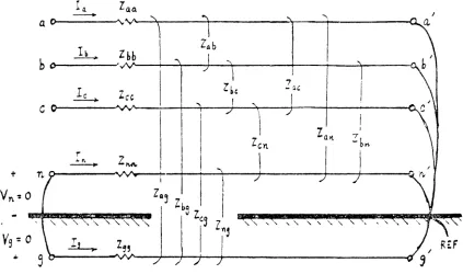
Two segments of parallel wires (denoted by a-a' and b-b') are

shown in Figure 3-2. This particular circuit model will be used to

describe self and mutual inductance terms of the per-unit length

impedance matrix [2]. The circuit model is analogous to a one-turn

air core transformer equivalent. From field theory, if an applied

potential V creates a current I in the direction shown, a

mag-aa a

netic flux ~ba linking coil 'b' due to the current in 'aT will be

established. Lenz's law states that a counterflux ~ab will oppose

~ba' thus creating an induced current in the direction b-b'. Thus,

a mutual impedance term establishes the effective induced voltage in

the opposing wire, and the circuit equations may be written as:

V

a V 'a

v '

_b

<3.12>

<3.13>

Several

where Zaa

=

R

a a + jwLaa, and Zab = Ra b + jwLa b , etc.

references {31,32} show the computations for parallel cylindrical

wires. This involves the summation of partial self-inductance terms

~~

+'10(4.' - - - - _~ T

:l~Cl I

-0.-

_«

a

~

+ 0 _t

Va.

Vr;.,1

- .i-

o

-.-L

to..b :

t

htL

I _I

liLt-

---~

I.

-- ---T-- t

I

lH

I

b

Ib

~ j,'

+

G

I\IV' )

0 ₊

Vb Vb'

---L.

.L

where length of line's' is much larger than radius r, the inductance per

unit length is:

Lis 10-7/2 + 2x10-7{In(2s/r)-1} _<3.14>

Since the GMR for cylindrical wires is D

s

therefore express self-inductance as:

O.779r {5}, ~e can

L 2x10-7{In(2s/D )-l}

s <3.15>

Likewise, mutual inductance Mis determined from geometric mean

distance (D ) and is defined as: m

M 2xlO-7{In(2s/D )-l}

m <3.16>

Although the above formulas for self and mutual inductances imply that

they are functions of line length s, we shall see that these terms

"cancel out" when equivalent expressions for self and mutual impedances

Section 3.3 - Application of Carson's Line to the Derivation of the Per-Unit Length Impedance Matrix

The basis for describing wave propagation in overhead

conduc-tors with earth return was presented by J.R. Carson in 1926. Various

authors (11,30} have used Carson's line with earth return in

trans-mission line applications, such as zero-sequence impedance calculations

for fault analysis. Here, we will derive self and mutual impedance

terms using a rather heuristic approach in which earth return is used

in the circuit model. This involves the utilization of Carson's line

with earth return, as shown in Figure 3-3. An overhead wire of unit

length (denoted by length a-a') carries a conductor current I , and

a

returns through the earth through a ficticious "ground conductor"

beneath the surface of the earth (denoted by length g-g'). Similar to

the method of images, which is commonly used in the computation of

sequence capacitances, the earth is assumed to extend infinitely with

uniform resistivity. The distance between the overhead conductor and

the ficticious "ground conductor" is denoted by D . This distance

ag

is a function of earth resistivity p, and is adjusted so that the

calculated inductance is equal to that measured by test (30}. From

equations 3.12 and 3.13, we can represent Carson's line (Figure 3-3)

I _z

a. a aa I

.-.,.. a

+

r

v

a

D REF

ag

)

7

V

!

g

= -I a

J

+

---...

_~I Fictitious earth

3

return conductor

I,.

1 UNIT

·1· .

I

z ag

[Va - va'l= 'Zaa

lVg-Vg'j

: -, II

' -I

a J

<3.17>

Note that voltages V , V " V , and V ' are all referenced to ground.

a a g g

Thus, we know that V_g 0, and V ' - V '_{a g}

=

o.

Subtracting the two

equations enables us to solve for V :_a

V

a (zaa + Zgg - 2zag)1a Zaa aI

where Z_aa z + Z - 2z

aa gg ag Zaa denotes the "total" self

impedance of conductor "a" vith earth return accounted for, whereas ..

lower case z denotes the self-impedance of conductor "a" without aa

earth return. Z_aa can be regarded as the total self impedance, since

it contains an earth resistance term r ._g From equations 3.15 and

3.16, we can express each component of total self-impedance Z as:

aa

z aa

z gg

z ag

r

a + jOOk{ln(2s/Ds a)-1} Q/unit length

r + jwk{ln(2s/D )-1} Q/unit length

g sg

jwk{ln(2s/D_ag)-l} Q/unit length

<3.18>

<3.19>

<3.20>

where D_sa and D_sg denote self GMD's of conductors "a" and "(J""o ,

respectively. Combining terms from Equations 3.18, 3.19. and 3.20 and

Z

aa (Ra g e+ R ) + jwkln(D /Dsa) <3.21>

where D_e is commonly defined as D_e = D 2/ D {1l}. The parameter

ag sg

De is dependent upon both earth resistivity p and frequency!, and

is defined by:

D

e 2160(p/j)1/2 <3.22>

An identical methodology is followed for deriving a system of three

phase conductors ~ith or vithout ground wires. The derivation is shown

in Appendix A. Given the physical geometries and conductor

specifi-cations, it is possible to theoretically calculate per-unit length

impedance parameters. Factors such as skin effect can be estimated by

a method also shown in Appendix A and also in {22}.

Section 3.4 - Derivation of the Admittance Matrix

Just as magnetic field effects are considered for studying

inductance, the distribution of the electric fields determine the

capacitance of a system of parallel conductors. The shunt admittance

matrix [Y], as mentioned earlier, consists of conductance and

capacitive reactance terms. However, the conductance term is usually

Unknown and often uncontrollable factors such as changes in

atmos-pheric conditions, dirt, and corona contribute to leakage current

between conductors, which often make conductance impossible to

measure. Thus, we assume negligible conductance contribution at

at distribution voltages and consider only capacitance terms.

Capacitance between conductors is defined as charge per unit

of potential difference. It is dependent upon the size and spacing

of the conductors relative to each other and to an earth conducting

plane. Intuitively, we can visualize current, or the movement of

charge, to increase and decrease with the instantaneous value of the

alternating voltage impressed on the system. This is evident in

standing waves, where charging current flows even in the presence

of an open-circuit load, as we shall later investigate.

Recall from field theory that the potential difference

between tva points P₁ and P

_z

external to a linear charge density q

(see Figure 3-4) is equal to the integral of the potential gradient E:

J E-dx

J

(q/2n£x)-dx <3.23>

Thus, by superposition, for an n-wire system carrying charge

densities qa' qb,···,qn' located above a ground plane, the

difference in potential between any two wires will be the sum of

+q

-

...

/

f

I II

/

/

/

~

_/

/

/

'"

,..("

/ '

v .

aJ (1/2n8)(qa1n{Daj/r} + qbln{Dbj/Dba} +

+ ••• + q_nIn{D ./D_{nJ na}})

<3.24>

Section 3.5 - Effect of Earth on Capacitance

The presence of earth as a conducting medium must be

account-ed for when calculating capacitance. The assumption that the earth

is a perfect conductor of infinite extent in a horizontal plane will

enable us to understand the effects of a conducting earth on

capacitance calculations.

Consider a parallel two conductor system with earth return

as shown in Figure 3-5. The physical location of the conductors is

defined with respect to a coordinate system in which the earth plane

is used as the horizontal reference axis and the axis of symmetry of

the pole structure as a vertical reference. In charging the conductor,

the earth surface and conductor plane can be regarded as equipotential

surfaces, since the earth has a charge equal in magnitude to that of

the conductor but opposite in sign. Assuming the earth is of uniform

resistivity and infinite, its surface can be replaced by a ficticious

conductor of the same size and shape as the overhead conductor at a

di~tance equal to that of the overhead conductor to earth. This

en-tails that if the earth is removed and a charge equal and opposite to

pole structure

conductor j

/

I

I

/!

_!

)

I

I

d ..

1J

conductor i

earth

I

I

I

I

I

I

~

image of

conductor i

\

D .. \

1J

\

\

\

I

I

I

I

I

I

I

I

1

image of

conductor j

1

~

j

then the plane midway between the two occupies the same position as

the equipotential surface. This ficticious conductor, having charge

equal and opposite to that of the overhead conductor is called the

image conductor.

Thus, since calculations involve only lengths between

con-ductors and their respective image conductors, the admittance matrix

is dependent only upon the physical geometry of the conductors

relative to earth.

From equation 3.22, a system consisting of four overhead

conductors can be equivalently expressed in matrix form as:

V B B

ab B B

\

;' qa

1

a aa ac an !

Vb 1/2Jt£ B_ba B_bb B

bc Bbn

I

:: I

<3.25>

V_c B_ca B_{c b} B _Bcd

cc

V B B i

nb B B _qn

_J

n _{na nc nn}

where the elements of matrix [B] are determined by the geometry of the

conductors as follows from Figure 3.5:

B ..

1J 1n(D . .IJ/d .. }1J <3.26>

dij diIStance between 1.th and ' thJ con uctor ford (i~j)

radius of it h conductor for (i:j)

D.. distance between the jth conductor and the image of the ith

conductor.

Equation 3.25 can also be expressed in a form similar to equation 3.23:

vhere

[V] = 1/2n£[B] [1']

~

=

[qa qb qc qn]T

<3.27>

We can arbitrarily define a charge coefficient matrix [P] as:

[P]

=

(1/2Jt€)[B]

where [P]

=

[C]-I, since q

[V] = [P]['f]

cV and

<3.28>

<3.29>

To obtain the total per-unit length admittance matrix [Y], we apply the

following relations: From Ohm's law, the current vector [I] is:

[ I ] [Y] [V] <3.30>

Current is also defined as the derivative of charge vith respect to

time. Thus,

[ I ] d['f]/dt j

-r

'¥] <3.31>

[ I ]

Thus, from 3.30:

jw[C] [V] <3.32>

[Y] [1] [V]-l JW. p-1 jw(2nEB-1) <3.33>

The complete calculation of the per-unit length admittance matrix for

the actual test network is given in Appendix A for a four conductor

system (Three phase wires, one neutral) with earth return.

Section 3.6 - Experimental Determination of Hulticonductor Line Parameters

A measurement technique for determining the per-unit length

parameters of a multiconductor network is presented in {21}. It is

formulated in terms of measurable short and open-circuit line

impedances at a particular frequency. From transmission line theory

for single-phase lines, the short-circuit input impedance Z and

sc

open-circuit input impedance Z can be expressed in terms of

atten-oc

uation constant a, phase constant

a,

characteristic impedance Z , and

o

line length 1 as:

z

sc

z

_oc

Z tanht« + jS)l

o

Z cotht« + jf3)l o

<3.34>

Multiplying equations 3.34 and 3.35 and solving for Z we obtain:

a

Z

o {Zsc ocZ }1/2 <3.36>

The expression for propagation constant in terms of Z and Z is:

sc oc

y = ex + jS = (arctanh{Z IZ }1/2)/1

sc oc <3.37>

Similarly, for a multiconductor system consisting of{N' conductors

(excluding ground wire), the resulting expressions for the

short-circuit and open-short-circuit input impedance matrices are:

[tanh(fl)][Z ]

o

Inv[tanh(rl)]-[Z] o

Solving for Z we obtain:

o

<3.38>

<3.39>

[Z ]

o {[ Zsc]Inv[Zoc]}-1/2 [2sc] <3.40>

The propagation matrix [f] is expressed as:

[ f]

1/')

{arctanh([Z ]Inv[Z ]) ~}/l

Having obtained [Z ] and [f] from equations 3.40 and 3.41, we can

o

solve for [Z] and [Y] by the following relations {14):

[Z]

[ Y]

[f][Z] o

Inv[Z ]·[f]

a

<3.42>

<3.43>

Thus, from the knowledge of the input impedance matrices for

open-circuit and short-open-circuit load conditions, the multiconductor line

parameters [Z] and [Y] can be obtained.

A technique for measuring these input impedance matrices

is presented in {21}, where ratios of voltage to current are measured

by effectively "isolating" self and mutual impedance and admittance

terms at a chosen frequency. The reader is referred to {21} for a

detailed explanation of this measurement procedure and the results

for a four-conductor line.

This experimental method of calculating line parameters could

not be implemented in our tests because the network was not conducive

to the measurement of open-circuit and short-circuit input impedances.

Thus, the validity of the mathematical model can only be determined

Chapter 4 - Network and Test Description

In order to gain an understanding of carrier signal

propa-gation on multiconductor distribution lines, several tests ~ere

performed on actual de-energized distribution networks at Carolina

Power and Light's Distribution Automation Test Facility. The test

facility offers a controlled environment in which propagation

measurements of voltage and current as a function of distance can

be performed. The 23 kV test facility, which was constructed to

Carolina Power and Light's distribution engineering standards, is

composed of spans of single-phase and three-phase sections of line.

These spans can be configured into various lengths of three-phase

and single-phase "netTHorks" by controlling oil break switches located

at various "switching poles". A more detailed description of the

test facility is presented in {6}.

Section 4.1 - Test Set-Up and Measurements

Propagation measurements were performed by injecting a 25 kHz

carrier signal at the sending end of a multiconductor network and

measuring voltage and current magnitudes at approximately equidistant

intervals along the network. The 25 kHz frequency was also used in

previous OLe experiments {3,~} in order to "visualize" nodes and

antinodes in standing ~ave patterns. These signal nulls occur at

1.77 miles at 25 kHz. Due to the physical limitations of the network

(approximately four miles each of three-phase and single-phase sections

of line), about one-half of a wavelength can be plotted for either

the three-phase or single-phase spans, which should yield sufficient

information for standing vave analysis.

Although the test facility accommodates both single-phase

and three-phase sections of overhead and underground distribution

lines, only the overhead conductors were utilized. These conductors

are classified as #2 AVG aluminum, and are spaced according to

distri-bution standards (Refer to Figures A-2 and A-3 as shown in Appendix

A). The neutral conductor follows an intermittent grounding scheme,

where grounding occurs at each pole (located about 300 feet apart).

Figure 4-1 shows the experimental set-up for carrier injection

at the sending end of the network, where a function generator (HP

3311A) in series with a power amplifier (HP 467A) is used to generate

the 25 kHz sinusoidal carrier signal. The signal is coupled to the

phase (denoted by A,B,C) and neutral (N) conductors by twisted pair

16 gauge wires, which are clamped on to each of the overhead

conductors. A connection box (banana-type connectors) vas built to

select either single-phase injection on conductor A, or three-phase

injection on all phases A,B, and C. The peak-to-peak source voltage

used for the propagations tests was SO volts- At the receiving end,

16 guage twisted pair wire was also used for any loads which were to

HP 3311A Function Generator

HP 467A Pover

Amplifier

R

R lOkQ

Frequency

Counter (25 KHz)

/

TO PHASE B

Figure 4-1

Connection Box

to phase.

The actual voltage and current measurements were performed in

a bucket truck using a battery-operated portable dual-channel

oscillo-scope (Tektronix 305 DHM). The voltage probe was modified by attaching

large alligator-type clips to signal and ground leads of a coaxial

cable, enabling voltage measurement from phase to phase and phase to

neutral, simply by clamping on to the wires. The current measurements

were made using a combination of a Fluke current transformer (clamp-on

with 1000:1 turns ratio) and a Tektronix current probe (model P6021).

In order to compensate for the 1000:1 decrease in current, the output

current of the Fluke was increased by placing 500 turns (type 40 A~G

wire) of the Fluke's secondary to the primary side of the Tektronix

current probe. Thus, the calibrated net transformer ratio was

approx-imately 1.75:1 at 25 kHz. Currents were measured on phases A,B, and

C only, since Hemminger {3} showed that almost no current flowed on

the neutral conductor more than two pole spans (about 600 feet) from

the source.

Section 4.2 - Network Configurations and Boundary Conditions

Multiconductor propagation measurements of voltage and

cur-rent were performed on three diffecur-rent networks. These net~orks are

shovn in Figures 4-2, 4-3 and 4-4. "Network #1", as shown in Figure

4-2, consists of a homogeneous span of parallel conductors A,B,C,

~_._--- 3.59 miles _---~

I

a O~--~---..,O

b o---~

...--..---..-;---....

---=o

C O,..,~~-

...

I:.:III:I:lI----...

---_rj

n

(")c~---

...

o

source

Figure 4-2

TABLE 4-1 Boundary conditions for tests conducted on Network #1

# OF PHASES SOURCE LOAD

TEST # INJECTED CONDITIONS CONDITIONS

ZSA SQ ZLA OPEN

1

la 2

SB OPEN ZLB OPEN

(PHASE A)

ZSC OPEN ZLC OPEN

ZSA

=

5Q ZLA OPEN

Ib 3 2

SB 5Q ZLB OPEN

ZSC 5Q ZLC OPEN

ZSA SQ ZLA OPEN

1

lc _ZSB lOKQ

ZLB +jZol

(PHASE A)

ZSC lOKQ ZLC -jZ₀₂

ZSA 52 ZLA OPEN

Id 3 _ZSB SQ _{ZLB +jZol}

ZSC SQ _ZLC -jZ₀₂

2

corresponds to Figure 4-2, where the parallel conductors assume a

vertical geometry with phase A on top, B in the middle, and C on the

bottom, the closest to neutral conductor N. The total length of the

network is approximately 3.59 miles, or 18,962 feet. In a sense, the

network is symmetrical in that all conductors (A,B,C,N) span the same

total length, (i.e. there are no discontinuities that result from

unequal line lengths). Thus, this particular network is easily

modeled as one continuous, homogeneous section of line. In actuality,

this is not the case due to variations in conductor geometry

result-ing from transpositions, differresult-ing pole heights, etc. However, for

simplicity, we shall model this "symmetric" network as one continuous

section of line, characterized by the same set of distributed

per-unit values throughout.

A series of tests was made on Network #1 by applying

sev-eral combinations of boundary conditions at the source and load.

At the source, current was injected on either: (i) phase A only

(single phase injection), or (ii) on all phases A,B, and C

(three-phase injection). On the receiving end, load conditions were applied

as follows: (i) all phases A,B,C open, or (ii) phase A open, phase B

terminated in +jZ , and phase C terminated in -jZ (loads

connect-o 0

ed between phase and neutral). No phase to phase source or load

terminations were applied. The combinations of two source and two

load conditions resulted in a series of four independent tests

for example denotes the load impedance connected between phase A and

neutral. Likewise, ZSA denotes the source impedance connection between

A and N. The term "open" implies an open-circuited load.

Network #2, as shovn in Figure 4-3, is very similar to Network

#1 with the exception of phase A, which extends about 1.18 miles

further, spanning a total length of 4.77 miles. The lengths of Band

C are unchanged at 3.59 miles. The extension of phase A causes the

network to be asymmetric. Hence, a discontinuity exists in the

net-work, for which two sets of line parameters must be employed to the

multiconductor solution equations presented in Chapter 2. Some

interesting coupling phenomenon result from this discontinuity, as

we shall see in the next chapter. The source and load conditions

for this network and the corresponding test cases are summarized in

Table 4-2. Note that the load conditions change only for phase A.

Network #3, shown in Figure 4-4, adds another discontinuity

by effectively reducing the length of phase conductor C by one-half.

Here, we are interested in the effect of discontinuities (which result

from an open-circuit) on the propagation in each of the phase

conduc-tors. The three-phase netvork is reduced to a two-phase network after

propagating 1.82 miles, and is then further reduced to a single-phase

network after traveling 3.59 miles. Because the test facility is

composed entirely of single and three-phase distribution lines, a

"true" tl,rJo-phase system W'as not physically configurable. However, it

4.77 miles

!_,

"

3.59 miles

b o~---o

I

I

c o~---o

,

n

0---...0

i .. source load

I

~I

TABLE 4-2 Boundary conditions for tests conducted on Network #2

# OF PHASES SOURCE LOAD

TEST # INJECTED CONDITIONS CONDITIONS

ZSA = SQ ZLA SHORT

1

2a _ZSB OPEN _ZLB OPEN

(PHASE A)

ZSC OPEN ZLC OPEN

ZSA = SQ ZLA OPEN

1

2b _ZSB OPEN _ZLB OPEN

(PHASE A)

ZSC OPEN ZLC OPEN

ZSA SQ _ZLA SHORT

2c 3 _ZSB 5Q _ZLB OPEN

ZSC SQ ZLC OPEN

ZSA 5Q ZLA OPEN

2d 3 _ZSB 52 _{ZLB OPEN}

--- 4.77 miles

I ~ 3.59 miles

~._---_.

b O~---O

~ 1.82 miles ~

I

C

c...

---~o--n c,·~---~---~---.--.-(O

!

load--~

TABLE 4-3 Boundary conditions for tests conducted on Network #3

# OF PHASES SOURCE LOAD

TEST # INJECTED CONDITIONS CONDITIONS

ZSA SQ ZLA SHORT

1

3a _ZSB lOKQ _ZLB OPEN

(PHASE A)

ZSC lOKQ ZLC OPEN

ZSA

=

5Q _ZLA

₌

_OPEN

1

3b _ZSB lOKQ _ZLB OPEN

(PHASE A)

ZSC lOKQ . ZLC OPEN

ZSA

=

SQ ZLA 410

1

3c _ZSB lOKQ _ZLB OPEN

(PHASE A)

ZSC lOKQ ZLC OPEN

ZSA

=

5Q _ZLA SHORT

3d ')

ZSB SQ ZLB OPEN

..J

ZSC SQ ZLC OPEN

ZSA SQ ZLA OPEN

3e j

ZSB SQ '7 _OPEN

...) _L1

LB

ZSC SQ _ZLC OPEN

ZSA SQ ZLA 410Q

3f 3 _ZSB SQ

ZLB OPEN

wire physically exists with both ends open, and can therefore be

considered as an equipotential neutral conductor. Table 4-3

sum-marizes the various source and load boundary conditions that were

applied to Network #3. A total of six tests were conducted. Note

again that loads ZLB and ZLC at their receiving end remains open in

all test cases. The 10 kilohm source impedance was used to simulate

the impedance of a substation transformer {3}.

The results of all propagation tests are tabulated and

plotted in Appendix C. Because of the extensive amount of

experi-mental data, a few tests, particularly those which were conducive

to simulation, will be analyzed and commented upon in greater detail

Chapter 5 - Test Results and Analysis

The experimental and theoretical results of several test

cases are analyzed in the sections to follow. Because of the

ex-tensive amount of data from the various tests described in the last

chapter, only a few of the more significant results will be discussed.

Computer simulation results will be compared to empirical data to

check the validity of the mathematical model.

Because the solution process to the multiconductor problem

is so mathematically complex, it lends very little insight to the

actual physical occurrences along the distribution network.

Conse-quently, an analytical approach will be taken which involves the

application of transmission line fundamentals. The Smith chart, for

example, provides an accurate solution and a physical interpretation

of what happens on the line.

Section 5.1 - Experimental and Theoretical Results of Test lIb

(Bundled Conductor)

As described in Table 4-1, test case #lb was conducted on

a symmetric netvork, ~here each conductor spans a distance of

approx-imately 3.59 miles. For this particular test, three phases (A,B,C)

were injected with a 25 kHz sinusoid. At the load, all phases were

terminated in an open circuit. The standing wave patterns for voltage

A total of ten locations were chosen as measurement points. A spline function was used in plotting the subsequent standing wave patterns

for each phase. Note that the voltage minimum and current maximum

both occur approximately at the midpoint of the network, a

quarter-wavelength from the load. This is because the network length is very

close to an electrical half-wavelength at 25 kHz.

For a lossless line, a half-wavelength (\12) at 25 kHz

corresponds to a distance of 3.73 miles. From previous propagation

tests conducted by Hemminger {3}, the velocity of propagation of an

unloaded distribution line was measured to be 95% of the speed of

light in air, which indicates that the line is virtually loss less and

conducive to TEM, or quasi TEM modes of propagation. Thus, an

electri-cal half-vavelength adjusted for 95% speed of propagation is actually

about 3.54 miles, which is very close to the total netvork length of

3.59 miles. The symmetry of the standing wave patterns indicates that

the network is indeed very close to a half-wavelength.

Figure 5-1 shows the voltage standing wave pattern for phases

A, B, and C. Because of the uniformity of the network (all phases

being of equal length and all conductors uniform), we would

anti-cipate that all phases would exhibit identical standing ~ave patterns.

In essence, this particular three-phase system can be considered as a

single-phase bundled conductor, in which the three phases constitute

the bundle. As discussed in Chapter 3, a system of parallel wires

carrying unequal currents will mutually induce voltage on neighboring

PHASE TO fo'[UTRAl VOltAGES (T£ST,es) '0 to .0 , o L 10

,

S ao 10 ~~ ... I"

...

It .• .,. .

.... l." I." . . . . I.... ..M ,... 1.&1

o.04 0 40 0 ' .0 1. 20 I.60 2 . 00 J . I t I . " I. 19 J.Jt

DUrAlIIICI n . SOuUI (MIL'S)

Olst·JnC. fr'Olfo ~~ (",tlea)

PHASE CuRMNTS (TEST'I8)

'ea • -..----I

..

• ---- .

,

u

.

-....

r:

'" .' ; / .' ! ,-i \ \ \ \

\.~\

\

...

\ ... \ ~...-\ .110 .'70 .,Iot ..Jt

SIWULATED PHASE CURREKTS(TESTliB) C\S·('~t lA)

.'M

.,...

....

6 ...J

1. ...-,

...

-.

I

~

.

I

" " - - l S '~... ·

I

-,

~ ' . - t - + ' 0 ..···0 I ~,_.-A

o " , -A- ' ...

""~-'''

-.

. , . ' / , ,. > :D-<,~_..

,,/ / '0

,.'/,.,D

»<>_{. /}

a " "

:~

y'

70 '0 60 10 40 20 '0 10 10

0.00 0.40 0.10 r.20 1.60 Z. 00 2.J, 2.7f J. l ' 3. , .

DISUNCI "'OM SOURel (HILlS)

.... .... ..at .... .... ... •.•• J.lI 1.W

[Iht·:...:~ fr.jfA ~.:. (",1l~&)

lJ1

V1

'~ via current in phase \a~ producing an induced voltage across the

mutual inductance term Zab. In the case of a bundled conductor, or

any balanced three-phase circuit ~hereIIJ can be considered as the

superposition of equal currents I , I

b, and I , the flux linkages

a c

between phases will essentially be zero because the magnetic field

intensity H is zero. Thus, no mutual induction takes place. This is

evident in Figure 5-1, where all phase voltages are equal. The phase

to phase voltages were also measured to be zero, which justifies the

absence of mutual coupling effects on a uniform network.

The phase currents, as expected, are not exactly equal at all

points along the network. This can be attributed to the physical

geometry of the conductors. Although the network is considered to

be symmetric, other factors, such as unequal spacings between phases,

variations in conductor heights above ground (due to terrain), and

skin effect can cause unequal current division between homogeneous

conductors. Skin effect results in a decrease in current density

toward the center of the conductor. This inequality in current

density is caused by a longitudinal element near the center of the

conductor being surrounded by more magnetic lines of force, hence

reducing the net driving emf at the center element. Thus, virtually

all of the current is concentrated near the surface of the conductor.

In addition, the netvork experiences changes in conductor geometry

in the form of "tvists". These tvists involve the transposition of

afore-mentioned nonuniformities have some effect on voltage and current

distribution, and is the probable cause for the slightly different

standing wave patterns between the phase conductors shown in Figure

5-1.

Since this particular network can be treated as a single

bundled conductor, certain transmission line parameters such as

characteristic impedance and propagation constant can be evaluated

from empirical data. For single phase lines, the characteristic

impedance is obtained by the following relation:

z

_o (2 Z )1/2

sc oc

<5.1>

where Z represents the short-circuit input impedance, and 2

sc oc

the open-circuit input impedance. From Figure 5-1, the impedances

for short-circuit and open-circuit load conditions can be obtained

by assuming that the netvork length is equal to an electrical

half-wavelength. This assumption is valid due to the symmetry of the

standing wave patterns, as discussed before. Since voltage and

cur-rent minimas and ~aximas repeat every half-wavelength, the input

impedance for this symmetrical network can be represented by:

I

v

II

I

oc oc

12

I

375 ohms

o

55 volts/12.3 rna

7 volts/222.2 rna

4.47 kohms

The open circuit input impedance is obtained at the end of the line,

where V

=

V ,and current I = I .

=

I + I

b + I .

Like-oc max oc mIn a c

wise, the input impedance looks like a short circuit at the midpoint

of the network where V = V . , and I = I

sc mIn sc max Note that

the currents for both short-circuit and open-circuit loads are the

superposition of individual currents flowing in each of the phase

conductors. Hence, we see that the input impedance is dependent upon

line length. Because this particular network is one-half wavelength

long, the input impedance always "looks" like the load impedance. If,

however, the network length were ~ quarter-wavelength, then the input

impedance for an open-circuit load would look like a short.

The empirical value for characteristic impedance 2 of

o

375 ohms is consistent with that derived theoretically for a bundled

conductor. The theoretical value for Z of 372 ohms is derived

o

in Appendix B, and is based on methods described in Chapter 3 for

computing per-unit length matrices [Z] and [Y]. From a previous

experiment conducted on an unloaded single phase network {3}, 2

0

was measured to be in the neighborhood of 450 ohms. The decrease in

Z for a bundled conductor is expected since the equivalent

geomet-o

ric mean radius is greater than that of a single conductor. Hence,

the inductance is decreased with the addition of conductors, while

the capacitance to ground is increased, which results in a net

de-crease in the magnitude of the characteristic impedance.

maxima for each phase conductor all occur at the same location

with respect to the load (midpoint of the network), we may deduce

that the propagation constant (y

=

a + jS) for each conductor

is the same. Furthermore, the propagation matrix

r

is diagonal.

Recall from Chapter 2 that the propagation matrix contains elements

(eigenvalues) that define the modes of propagation. It is evident

from Figure 5-1 that the imaginary components

<a ,

_a

a,

_~b

a )

_c of the

propagation constant are equal.

A simulation program based on the mathematical model presented

in Chapter 2 was written by M. Riddle {33). Several test cases were

simulated for comparison vith empirical results. Figure 5-2 shows the

theoretical standing wave patterns generated for the symmetric network

denoted by test #lb. The per-unit length parameters, namely the [Z]

and [Y] matrices were derived by the methodology described in Chapter

3. These parameters are derived in Appendix A for the test network

used in making the propagation measurements. In comparing the measured

data (Figure 5-1) to that of the theoretical (Figure 5-2), we see

noticeable differences, the most prominent being the lack of symmetry

in Figure 5-2. Another discrepancy between the two plots exists in

the phase voltages being unequal in Figure 5-2, ~hereas the measured

voltage standing wave patterns in Figure 5-1 are identical.

There are several possible explanations for these apparent

differences. The first is that the theoretically derived per-unit

length parameters do not accurately represent the actual test network

reality, this is not the case. Many approximations were made due to

uncertainties in the network parameters. For example, the physical

geometry of the conductors changes throughout the netVlork from

"verti-cal" to "delta" configurations, as mentioned previously. These

conductor t~ists, which cannot be regarded as a true transposition

in a strict sense, have an effect similar to that of a complete

transposition cycle in that the rotating of conductors effectively

reduces, or "cancels out" mutual impedance effects. In the derivation

of the per-unit length impedance matrix, these twists were not taken

into account. Other uncertainties, such as conductor heights are

inherent in varying terrain levels. In addition, non-uniform conductor

spacings, and earth resistivity also have an effect on signal

propaga-tion. These "non-uniformities" in the network could affect the

calculated parameters [Z] and [Y], but their sensitivity to these

non-uniformities is not yet knoVln. However, based on several "trial

and error" variations of line length, the experimental standing

wave-forms could be matched. In particular. the network seemed especially

sensitive to line lengths corresponding to multiples of

quarter-wavelengths, vhich is the case in test #lb.

Another possible source of error could be attributed to lack

of precision in the numerical solution process. Since the computer

simulation involves matrix functions (multiplication, diagonalization,

inversions, etc.) vhich are used iteratively, a very slight error in