During Early Building Design. (Under the direction of Joseph DeCarolis, and Edward Jaselskis.)
Much of our global energy supply is ultimately consumed in buildings. In the U.S., buildings account for approximately 40% of domestic energy consumption. While significant opportunities exist to improve building energy performance, inflexibility and lack of
practically effective energy assessment tools available for use during the early design process limit opportunities to explore energy efficient design alternatives. Particularly in the early stages of building design, when key decisions can have a strong effect on realized energy performance, architects lack tools that can inform building design with energy performance data. While energy simulation engines exist, they require the specification of relatively detailed building plans that require significant effort and time to setup and run; therefore such models are typically applied late in the design process to verify energy performance. As a result, building energy performance has served as a design outcome rather than a design goal.
A previous study used EnergyPlus, a whole building energy simulation engine, within a Monte Carlo simulation framework to develop a linear regression-based building energy model (LRBEM) that can predict building energy performance based on the specification of 27 parameters relevant to the early building design phases. The model was limited to
medium-sized U.S. commercial office buildings with rectangular geometries in four different climate zones represented by the cities of Miami, Winston-Salem, Albuquerque, and
Minneapolis. The goal of this thesis was to extend the applicability of the previously
the accuracy of the LRBEM was inconsistent across different building geometries, the model was reformed to include building wall area as an explanatory variable, which significantly improved its predictive capability. The revised model, LRBEM+, was exercised on a set of limiting cases designed to systemically test variations in building geometry. Finally, LRBEM+ was tested to examine how well it responds to changes in individual design parameters. With the exception of heating in Miami, the R² values obtained from the
by
Maged F. Al Gharably
A thesis submitted to the Graduate Faculty of North Carolina State University
in partial fulfillment of the requirements for the degree of
Master of Science
Civil Engineering
Raleigh, North Carolina 2013
APPROVED BY:
_______________________________ ______________________________
Joseph DeCarolis Edward Jaselskis
Committee Co-Chair Committee Co-Chair
________________________________ ________________________________
DEDICATION
BIOGRAPHY
ACKNOWLEDGMENTS
When thinking about names to thank, a lot of them come to my attention. I would like to start by thank Allah for all his blessing and generosity.
To my parents and family, thank you for your love, support and advice throughout my academic career and standing by my side during my best and worst times.
To my advisers, Drs. DeCarolis and Ranjithan: you have been great mentors and supporters. Your efforts have never gone unappreciated and you have helped me out more than you know, I deeply appreciate it.
To Dr. Jaselskis and Liu, thank you for the great knowledge and advice. Our in class discussions and office visits were off great help in directing my career path and shaping my future.
I would also like to acknowledge the other people, whose discussion and
TABLE OF CONTENTS
LIST OF TABLES ... vi
LIST OF FIGURES ... viii
CHAPTER 1 INTRODUCTION ... 1
CHAPTER 2 MODEL DEVELOPMENT ... 5
2.1. Prior Model Development ... 5
2.2 Initial Investigations to Test Applicability of LRBEM to New Building Geometries ... 7
2.3 Development and Testing of a New Linear Regression-based Building Energy Model (LRBEM+). ... 10
CHAPTER 3 LRBEM+ APPLICATIONS TO BUILDINGS WITH DIFFERENT CONFIGURATIONS ... 17
3.1 LRBEM+ performance assessment procedure ... 17
3.2 Non-rectangular-shaped buildings with right-angled corners ... 17
3.3 Buildings with one different shape factor ... 18
3.4 A building with many different shape factors ... 25
CHAPTER 4 OUTCOME AND DISCUSSION ... 32
REFERENCES ... 34
CHAPTER 5 APPENDICES ... 36
Appendix I ... 37
Appendix II ... 38
Appendix III ... 39
Appendix IV ... 40
LIST OF TABLES
TABLE 2.1:BUILDING DESIGN PARAMETERS RELEVANT TO THE EARLY DESIGN STAGES. ... 5
TABLE 2.2:METHODS USED TO ESTIMATE HEATING AND COOLING LOADS USING THE EXISTING,
UNMODIFIED LRBEM ... 9
TABLE 2.3:CHANGES IN THE SET OF PARAMETERS CONSIDERED IN THE NEW REGRESSION MODEL ... 11 TABLE 2.4:LRBEM+ PERFORMANCE IN PREDICTING HEATING ENERGY LOADS FOR BUILDINGS
IN FOUR CLIMATE ZONES; THE ERRORS REPRESENT THE DIFFERENCE BETWEEN LRBEM+
PREDICTIONS AND ENERGYPLUS SIMULATIONS. ... 12
TABLE 2.5:LRBEM+ PERFORMANCE IN PREDICTING HEATING ENERGY LOADS FOR BUILDINGS IN FOUR CLIMATE ZONES; THE ERRORS REPRESENT THE DIFFERENCE BETWEEN LRBEM+
PREDICTIONS AND ENERGYPLUS SIMULATIONS ... 13
TABLE 2.6:COMPARISON BETWEEN HEATING IN MIAMI AND WINSTON-SALEM FOR THE
VERIFICATION SET, ENERGY VALUES ARE OBTAINED FROM THE LRBEM+ ... 16
TABLE 3.1:PREDICTION MEAN-BIASED ERROR FOR HEATING AND COOLING IN THE FOUR
TABLE 5.1:FINAL CROSS PRODUCT PARAMETERS, AS WELL AS THEIR VALUES THAT WERE INCLUDED IN THE HEATING EQUATION FOR THE MULTIVARIATE REGRESSION MODEL ... 41
TABLE 5.2:FINAL CROSS PRODUCT PARAMETERS, AS WELL AS THEIR VALUES THAT WERE INCLUDED IN THE COOLING EQUATION FOR THE MULTIVARIATE REGRESSION MODEL ... 43
TABLE 5.3:LIST OF BUILDING PARAMETERS AND DERIVED PARAMETERS THAT WENT INTO THE
STEPWISE REGRESSION ... 45 TABLE 5.4:BUILDING 1 PARAMETER DEFINITIONS. ... 48
TABLE 5.5:EXPERIMENTS A THROUGH C PARAMETER DEFINITIONS. ... 48 TABLE 5.6:RANKING OF THE 30 PARAMETERS ACCORDING TO THEIR IMPORTANCE IN HEATING
IN THE FOUR CLIMATE ZONES, KNOWING THAT THE IMPORTANCE OF WALL, ROOF, FLOOR
AREAS ARE AGGREGATED WITH AREAS.. ... 50 TABLE 5.7:RANKING OF THE 30 PARAMETERS ACCORDING TO THEIR IMPORTANCE IN COOLING
IN THE FOUR CLIMATE ZONES, KNOWING THAT THE IMPORTANCE OF WALL, ROOF, FLOOR
LIST OF FIGURES
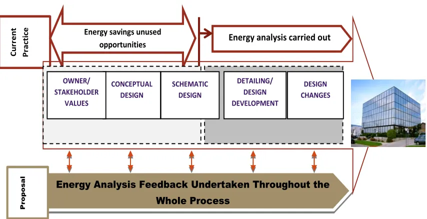
FIGURE 1.1:CURRENT PRACTICE IN WHICH ENERGY ANALYSIS TAKES PLACE NEAR THE END OF THE DESIGN PROCESS CONTRASTED WITH PROPOSED PRACTICE WHERE ENERGY ANALYSIS
TAKES PLACE THROUGHOUT THE BUILDING DESIGN PROCESS ... 3
FIGURE 2.1:THESE SCATTER PLOTS SUGGEST A STRONG LINEAR RELATIONSHIP FOR THE 4000 INSTANCE EXPERIMENTS OBTAINED BY COMPARING BETWEEN THE COOLING AND HEATING ENERGY PERFORMANCES OBTAINED BY LRBEM+(HORIZONTAL AXIS) AND ENERGYPLUS (VERTICAL AXIS). ... 14
FIGURE 3.1:AN EXAMPLE OF A RECTILINEAR-SHAPED NON-RECTANGULAR BUILDING WITH RIGHT-ANGLED CORNERS THAT WAS USED TO TEST THE PREDICTABILITY OF LRBEM+. . 18
FIGURE 3.2:AN EXAMPLE BUILDING WITH OPEN AREAS IN THE MIDDLE THAT CAUSE SELF -SHADING EFFECTS (CASE A-1: A SMALL COURT YARD) ... 19
FIGURE 3.3:AN EXAMPLE BUILDING WITH OPEN AREAS IN THE MIDDLE THAT CAUSE SELF -SHADING EFFECTS (CASE A-2: A LARGE COURT YARD). ... 19
FIGURE 3.4:AN EXAMPLE BUILDING WITH CORNERS THAT ARE NOT RIGHT ANGLED (CASE B-1: CORNERS WITH ACUTE ANGLES) ... 20
FIGURE 3.5:AN EXAMPLE BUILDING WITH CORNERS THAT ARE NOT RIGHT ANGLED (CASE B-2: CORNERS WITH OBTUSE ANGLES). ... 20
FIGURE 3.6:AN EXAMPLE BUILDING WITH NON-UNIFORM ROOF HEIGHTS (CASE C-1) ... 20
FIGURE 3.7:AN EXAMPLE BUILDING WITH NON-UNIFORM ROOF HEIGHTS (CASE C-2). ... 21
FIGURE 3.9:WINSTON-SALEM ABSOLUTE PERCENTAGE ERROR VERSUS FLOOR-TO-FLOOR HEIGHT.PERCENTAGE ERROR WAS OBTAINED BY COMPARING ENERGY PREDICTIONS FROM THE LRBEM+ WITH ENERGYPLUS SIMULATION RESULTS. ... 24 FIGURE 3.10:A BUILDING WITH SEVERAL SHAPE FACTORS SIMULTANEOUSLY CHANGED TO
DEVIATE FROM THE PURE RECTANGULAR-SHAPED BUILDING (CASE E). ... 25
FIGURE 3.11:COMPARISON OF RELATIVE CHANGE IS COOLING AND HEATING ENERGY LOADS
(FOR MIAMI) PREDICTED BY LRBEM+(RED) AND ENERGYPLUS (BLUE) IN RESPONSE TO INCREMENTAL CHANGE (TABLE 7) IN EACH BUILDING PARAMETER.PARAMETERS ON X
-AXIS ARE RANKED BY LEVEL OF IMPORTANCE (LEFT BEING MOST INFLUENTIAL). ... 28
FIGURE 3.12:COMPARISON OF RELATIVE CHANGE IS COOLING AND HEATING ENERGY LOADS
(FOR WINSTON-SALEM) PREDICTED BY LRBEM+(RED) AND ENERGYPLUS (BLUE) IN RESPONSE TO INCREMENTAL CHANGE (TABLE 7) IN EACH BUILDING PARAMETER.
PARAMETERS ON X-AXIS ARE RANKED BY LEVEL OF IMPORTANCE (LEFT BEING MOST INFLUENTIAL). ... 29
FIGURE 3.13:COMPARISON OF RELATIVE CHANGE IS HEATING ENERGY LOAD (FOR
ALBUQUERQUE) PREDICTED BY LRBEM+(RED) AND ENERGYPLUS (BLUE) IN RESPONSE TO INCREMENTAL CHANGE (TABLE 7) IN EACH BUILDING PARAMETER.PARAMETERS ON X -AXIS ARE RANKED BY LEVEL OF IMPORTANCE (LEFT BEING MOST INFLUENTIAL). ... 30 FIGURE 3.14:COMPARISON OF RELATIVE CHANGE IS HEATING ENERGY LOAD (FOR
INCREMENTAL CHANGE (TABLE 7) IN EACH BUILDING PARAMETER.PARAMETERS ON X
-AXIS ARE RANKED BY LEVEL OF IMPORTANCE (LEFT BEING MOST INFLUENTIAL). ... 31
FIGURE 5.1:FRAMEWORK OF METHOD “COMBINATION OF RECTANGLES”. ... 37
FIGURE 5.2:FRAMEWORK OF METHOD “PERIMETER PRESERVED”. ... 38
FIGURE 5.3:THE FRAMEWORK FOR “FLOOR AREA PRESERVED”. ... 39
Chapter 1
Introduction
In 2011, approximately 41% of total U.S. energy consumption (equivalent to 40 quadrillion BTU) was consumed in buildings (US EIA, 2012). This is equivalent to more than nearly18 times the total energy produced in the African continent for the year 2009 (US EIA, 2010). Significant potential for energy savings exist by optimizing building design in a way that minimizes the thermal cooling and heating loads, which constitute a major portion of the total energy consumed by buildings. Formal consideration of energy performance has typically been addressed by engineers in the later stages of the design process when much of the building design is already fixed. Thus building energy performance is currently viewed mostly as a design outcome rather than as a design target.
The AIA describes Building Energy Modeling (BEM) as a tool to predict the anticipated building energy usage and as a method to capture the corresponding energy savings compared to a baseline (AIA, 2012). However, utilizing the available suite of building energy simulation tools requires substantial time, information, and technical expertise that make effective use of BEM infeasible for architects in the early design stages. With increasing attention to energy performance modeling, design professionals are
design phase. Consequently, most design decisions that greatly influence building energy performance are frequently made in the absence of model-based energy estimates.
A recent study by the Association of Collegiate Schools of Architecture (ACSA) showed that most architects acknowledge the importance of interoperability between energy simulations and design (AIA, 2012). The AIA study calls for simplified simulation methods and/or improved user-interfaces for complex building energy simulation engines that are appropriately responsive to key early design variables. Such efforts could improve building energy performance by integrating energy analysis into all stages of design, as shown in Figure 1.1. Some notable efforts, such as ISO 13790 and MIT Design Advisor (Urban & Glicksman, 2007), have attempted to reduce the number of required inputs and to simplify the underlying model physics. A more recent approach, developed by Hygh et al. (2012), utilizes EnergyPlus, an existing whole building energy simulation engine, within a Monte Carlo framework to develop a linear regression-based building energy model (LRBEM) based on 27 building parameters relevant to the early design stages. The resultant LRBEM accurately predicts the energy performance of medium-sized, rectangular office buildings within four different U.S. climate zones represented by Miami, Winston-Salem,
Figure 1.1: Current practice in which energy analysis occurs near the end of the design process contrasted with proposed practice where energy analysis occurs throughout the building design process.
This thesis expands on the work described by Hygh et al. (2012) and Hygh (2011) by testing and extending the functionality of the LRBEM. This thesis meets three research objectives: (1) test the existing LRBEM’s accuracy in predicting energy loads for non-rectangular building geometries, (2) modify the LRBEM to better capture variation in building geometry, and (3) test the model’s accuracy in capturing the effect of changes in early design parameters on building heating and cooling loads.
The thesis is organized as follows. Section 2 describes the overall approach to extend the LRBEM to capture non-rectangular geometries and to test the model’s ability to capture changes in early design parameters. Section 3 presents results associated with the
Energy Analysis Feedback Undertaken Throughout the Whole Process
Pr
o
p
o
s
a
l
C
u
rr
e
n
t
Pr
ac
ti
ce Energy savings unused Energy analysis carried out
opportunities
Preconstruction
Constructio
n
CONCEPTUAL DESIGN
DETAILING/ DESIGN DEVELOPMENT SCHEMATIC
DESIGN OWNER/
STAKEHOLDER VALUES
Chapter 2
Model development
2.1. Prior Model Development
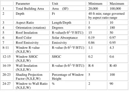
The work in this thesis builds on previous work by Hygh (2011) and Hygh et al. (2012), which describe the development of the original LRBEM. In this previous work, 27 building design parameters relevant to the early architectural design process were selected. For reference, these parameters are provided below in Table 2.1
Table 2.1: Building design parameters relevant to the early design stages.
Parameter Unit Minimum Maximum
1 Total Building Area Area (SF) 20,000 100,000
2 Depth Ft 40 ft min; range governed
by aspect ratio range
3 Aspect Ratio Length/Depth 1 10
4 Orientation (rotation) Degrees 0 180
5 Roof Insulation R-value(h∙ft2∙°F/BTU) 15 50
6 Roof Color Solar Absorptance 0.19 0.97
7 Roof Emissivity Emissivity 0.86 0.95
8-11 Window R-value (N,S,E,W)
R-value (h∙ft2∙°F/BTU) 1.1 4.3 12-15 Window SHGC
(N,S,E,W)
SHGC 0.2 0.6
16-19 Wall Insulation (N,S,E,W)
R-value (h∙ft2∙°F/BTU) R-8 R-40
20-23 Shading Projection Factor (N,S,E,W)
Percentage of Window Height
5 100
24-27 Window to Wall Ratio (N,S,E,W)
While the design parameters listed in Table 2.1 are likely to have a strong effect on building energy performance, several other factors, including prevailing climate, building size, and geometry, are also likely to exhibit a strong effect. While these factors could be included in the regression as explanatory variables, their addition to the model makes the regression significantly more complex and is likely to reduce the model’s predictive skill. As a result, Hygh (2011) made a set of assumptions exogenous to the model. A separate
LRBEM was developed for four different U.S. climate zones as defined by (ASHRAE, 2007), which were selected to capture climatic extremes. Weather files from the following representative cities were utilized: Miami, FL (Zone 1A), Winston-Salem, NC (Zone 4A), Albuquerque, NM (Zone 4B), and Minneapolis, MN (Zone 6A). In addition, while building size is an explanatory variable in the LRBEM, it is limited to the range associated with a U.S. medium-size commercial office building type drawn from the DOE Commercial Reference Building Models (Deru, 2011). This particular building type was chosen based on its ubiquity in the U.S. commercial building market. Building geometry was limited to rectangular
shapes, defined by building depth and aspect ratio.
used to create 20,000 building model instances, which were run through EnergyPlus to produce estimates of idealized heating and cooling loads for each model instance. A stepwise linear multivariate regression model was developed using 16,000 model instances, and the remaining 4,000 instances were used to verify the model. In addition to the early design parameters, several derived parameters were developed to increase the accuracy of the model. For example, total window area, based on the product of wall area and window-to-wall ratio, could potentially explain some of the variance in building energy performance. This enabled the inclusion of potentially useful non-linear terms in a linear regression model. Both the original 27 early building design parameters and derived parameters were treated as potential explanatory variables in the stepwise regression model. The stepwise regression procedure added explanatory variables to the regression model if it reduced the residual error in model prediction. A separate LRBEM was developed to predict heating, cooling, and total loads in each of the four climate zones, resulting in 12 separate regression models.
Parameters included and excluded by stepwise regression procedure are provided in the appendix to Hygh et al. (2012). Building design parameters and the additional parameters derived from them became explanatory variables in the LRBEM if retained by the stepwise regression.
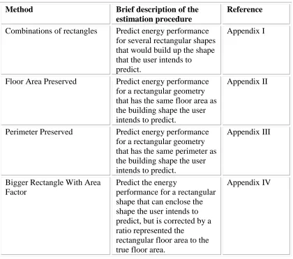
Table 2.2: Methods used to estimate heating and cooling loads using the LRBEM developed by Hygh et al. (2012).
Method Brief description of the
estimation procedure
Reference Combinations of rectangles Predict energy performance
for several rectangular shapes that would build up the shape that the user intends to predict.
Appendix I
Floor Area Preserved Predict energy performance for a rectangular geometry that has the same floor area as the building shape the user intends to predict.
Appendix II
Perimeter Preserved Predict energy performance for a rectangular geometry that has the same perimeter as the building shape the user intends to predict.
Appendix III
Bigger Rectangle With Area Factor
Predict the energy
performance for a rectangular shape that can enclose the shape the user intends to predict, but is corrected by a ratio represented the
rectangular floor area to the true floor area.
Appendix IV
correlated to floor and roof areas for a given building aspect ratio (i.e., length of the shorter side of the rectangular floor area divided by that of the longer side). In the LRBEM, the wall properties (such as wall area, window-to-wall ratio, R-value) were assumed to be the same for all sides of the building. As a result, the wall parameters were represented in the LRBEM by a single set of variables that were not specific to the wall in each cardinal direction. These observations led to a reexamination of the LRBEM model structure (i.e., the explanatory variables that describe the energy load). The following section describes the development and testing of an improved LRBEM.
2.3 Development and Testing of a New Linear Regression-based Building Energy Model (LRBEM+).
The simulation data used to develop the original LRBEM were used to develop a revised regression model, LRBEM+, which included five new parameters: wall area by cardinal direction and roof area. This approach enabled the development of a revised model without redoing the EnergyPlus simulation conducted by Hygh et al. (2012). For each of the four climate zones, the stepwise linear regression procedure (using the StepWiseFit function in MATLAB) was applied to the dataset consisting of 80% (16,000) simulations, chosen randomly, out of the complete set the 20,000 energy simulations. The remaining 4,000 the simulations were saved to conduct the model testing and performance assessment.
variables in the linear regression model (see Table 5.3 in the Appendix). The 30 building design parameters include 25 of the original 27 parameters from Hygh et al. (2012): aspect ratio and depth parameters were excluded but roof area and wall areas by cardinal direction were added. Details on the new explanatory variables in LRBEM+ are provided in Table 2.3
.
Table 2.3: Changes in the set of parameters considered in the new regression model.
Parameter Original LRBEM LRBEM+
Aspect
ratio 𝐿𝑒𝑛𝑔𝑡ℎ
𝐷𝑒𝑝𝑡ℎ
Excluded
Depth The shorter dimension in the rectangular floor plan
Excluded Wall Areas
(N,S,E,W)
𝐹𝑙𝑜𝑜𝑟 𝐴𝑟𝑒𝑎
𝑠𝑡𝑜𝑟𝑖𝑒𝑠 𝑑𝑒𝑝𝑡ℎ
𝐹𝑙𝑜𝑜𝑟 𝐴𝑟𝑒𝑎
𝑠𝑡𝑜𝑟𝑖𝑒𝑠
𝑑𝑒𝑝𝑡ℎ∗𝑎𝑠𝑝𝑒𝑐𝑡 𝑟𝑎𝑡𝑖𝑜 (
𝐹𝑙𝑜𝑜𝑟𝐴𝑟𝑒𝑎
𝑆𝑡𝑜𝑟𝑖𝑒𝑠 𝐷𝑒𝑝𝑡ℎ
)
∗ 4.571∗ 𝑠𝑡𝑜𝑟𝑖𝑒𝑠
( 𝐹𝑙𝑜𝑜𝑟𝐴𝑟𝑒𝑎𝑆𝑡𝑜𝑟𝑖𝑒𝑠
𝐷𝑒𝑝𝑡ℎ∗𝐴𝑠𝑝𝑒𝑐𝑡 𝑅𝑎𝑡𝑖𝑜
)
∗ 4.57 ∗ 𝑠𝑡𝑜𝑟𝑖𝑒𝑠
Roof Area 𝐴𝑟𝑒𝑎
𝑁𝑢𝑚𝑏𝑒𝑟 𝑜𝑓 𝑆𝑡𝑜𝑟𝑖𝑒𝑠
𝐹𝑙𝑜𝑜𝑟𝐴𝑟𝑒𝑎 𝑆𝑡𝑜𝑟𝑖𝑒𝑠
For each climate zone, the resulting regression model, based on the 16,000 data points, consisted of a reduced set of explanatory variables identified by the stepwise regression process; 48 explanatory variables were included in the final model for heating load and 35 explanatory variables in the model for cooling load. See Table 5.1and Table 5.2 in the Appendix for the resulting sets of explanatory variables and their corresponding
1 The 4.57 represents the metric floor to floor height that was used in the baseline model of the Monte Carlo
coefficients for heating and cooling, respectively, in each climate zone. For the datasets used for the model development, the LRBEM+ prediction for heating energy load in each climate zone yielded an R2 value between 0.765 and 0.965, and for cooling a value between 0.956 and 0.9926. The test datasets (i.e., the random set of 4,000 energy simulations not used in the LRBEM+ development) were used to first evaluate the ability of the newly developed regression models to predict the energy loads for rectangular buildings. The energy loads predicted with LRBEM+ were compared against the corresponding EnergyPlus simulation results. Table 2.4 and Table 2.5 show the values for coefficient of variance of root mean square error (CVRMSE), average percent error, and R2 for heating and cooling regression equations.
Table 2.4:LRBEM+ performance in predicting heating energy loads for buildings in four climate zones; the errors represent the difference between LRBEM+ predictions and EnergyPlus simulations.
Location Miami Winston-Salem Albuquerque Minneapolis
Climate Zone 1A 4A 4B 6A
R-squared 0.765 0.9584 0.9359 0.9645
RMSE (GJ) 1.6 28.8 44.2 74.1
CV (RMSE) 71.90% 9.50% 12.50% 5%
Mean Absolute Error 123% 7.8% 10.9% 6.1%
Table 2.5: LRBEM+ performance in predicting cooling energy loads for buildings in four climate zones; the errors represent the difference between LRBEM+ predictions and EnergyPlus simulations.
Location Miami
Winston-Salem
Albuquerque Minneapolis
Climate Zone 1A 4A 4B 6A
R-squared 0.9926 0.980 0.956 0.9715
RMSE (GJ) 31.2 27.1 34.7 203.0
CV (RMSE) 3% 5.70% 8.70% 6.80%
Mean Absolute Error
2.6% 4.7% 7.0% 5.8%
Miami Cooling Miami Heating
Winston Salem Cooling Winston-Salem Heating
Albuquerque Cooling Albuquerque heating
Minneapolis Cooling Minneapolis Heating
Figure 2.1: Scatterplots demonstrating the linear relationship between LRBEM+ (horizontal axis) and EnergyPlus (vertical axis) predictions for cooling (left column) and heating loads (right column). Each of the 4 rows represents results from one of the test locations.
R² = 0.9925 0
1000 2000 3000
0 500 1000 1500 2000
R² = 0.7639
-10 0 10 20
0 5 10 15
R² = 0.9801 0
500 1000 1500
0 500 1000
R² = 0.9584 0
500 1000 1500
0 500 1000 1500
R² = 0.9557 0
500 1000
0 500 1000
R² = 0.9368 0
500 1000 1500
0 500 1000 1500
0 500 1000
0 200 400 600 800
R² = 0.9645 0
2000 4000 6000
The LRBEM+ was able to predict more complex, non-rectangular building forms by considering 30 parameters in the stepwise regression, yet did not add more than 3% to the mean absolute error in cooling or heating at any location. Moreover, the addition of derived parameters and the displacement of some of the original design parameters in the stepwise regressions indicate that the new interaction between wall, window, and roof areas with their material properties is significant and should be accounted for in this analysis.
Table 2.6: Comparison between heating in Miami and Winston-Salem for the verification set; energy values were obtained using LRBEM+.
Heating Miami (Mwh) Heating in Winston-Salem (Mwh)
First Quartile 0.0591 43.3
Average 0.315 64.9
Chapter 3
LRBEM+ applications to buildings with different
configurations
3.1 LRBEM+ performance assessment procedure
This section describes the extended testing that was conducted to assess the performance of LRBEM+. Three types of testing were carried out: (1) rectilinear buildings; (2) buildings with a limiting shape factor as described in Section 3.3 (e.g., angle of building corners, non-uniform floor area in each story); and (3) a building that has a combination of shape factors. The following sections describe the applications of LRBEM+ to each of these cases and compare its prediction performance with energy values obtained using EnergyPlus.
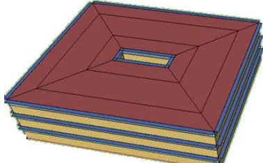
3.2 Non-rectangular-shaped buildings with right-angled corners
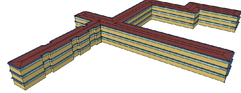
Several different rectilinear-shaped buildings with right-angled corners were
modeled and their heating and cooling energy loads in the four climate zones were estimated using EnergyPlus. An example of such a building is shown in Figure 3.1. The parameter values for all these buildings were chosen to be within the ranges (Table 2.1) used for generating the rectangular buildings that formed the datasets for developing the regression models. This ensured that the prediction performance could then be attributed to only the changes in the shape (i.e., purely rectangular to non-rectangular rectilinear). Overall
Table 2.4 and Table 2.5. For the example building shown in Figure 3.1, the mean-biased errors did not exceed 5%.
Figure 3.1: An example of a rectilinear-shaped, non-rectangular building with right-angled corners that was used to test the predictability of LRBEM+.
3.3 Buildings with one different shape factor
Figure 3.2: An example building with open areas in the middle that cause self-shading effects (Case A-1: a small court yard).
Figure 3.4: An example building with corners that are not right angled (Case B-1: corners with acute angles).
Figure 3.5: An example building with corners that are not right angled (Case B-2: corners with obtuse angles).
Figure 3.7: An example building with non-uniform roof heights (Case C-2).
Figure 3.8: Building A with non-uniform floor heights (Case D).
Cases A1 and A2 (Figure 3.2and Figure 3.3, respectively) represent two buildings with an interior courtyard with 3.9% and 15%, respectively, of the ground floor area. This deviation from a purely rectangular building leads to different amounts of self-shading on the building that could potentially affect the heating and cooling loads. The heating and cooling energy loads in the four climate zones for these two cases were estimated using LRBEM+ and EnergyPlus, and the prediction errors are shown in Table 3.1.
corners only. These cases have more than four corners, unlike the rectangular building that was used to generate the simulation data for LRBEM+. The prediction errors between
LRBEM+ and EnergyPlus estimates of energy loads for these cases are reported also in Table 3.1.
Cases C1 and C2, which include buildings with different roof heights, were also tested. The errors between energy load estimates by LRBEM+ and EnergyPlus are also shown in Table 3.1.
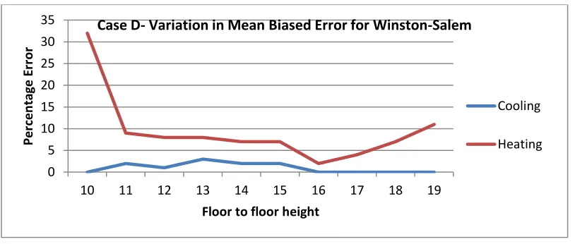
cooling and heating energy loads prediction errors with the floor-to-floor heights varying from 10ft to 19 ft. The graph suggests that LRBEM+ predicts the heating and cooling loads with acceptable error for the cases with floor to floor height between 11 ft. and 18 ft.
Table 3.1: Prediction mean-biased error for heating and cooling in the four climate regions for the different shape-factor cases A1, A2, B1, B2, C1, and C3.
Miami Winston-Salem Albuquerque Minneapolis Coolin
g
Heatin g
Coolin g
Heatin g
Coolin g
Heatin g
Coolin g
Heatin g A1
(Fig. 3.5)
1% - 7% 4% 4% 8% 8% 4%
A2 (Fig. 3.6)
2% - 4% 1% 4% 3% 2% 11%
B1 (Fig. 3.7)
2% - 4% 7% 18% 20% 10% 6%
B2 (Fig. 3.8)
3% 25% 4% 12% 7% 3% 8% 7%
C1 (Fig. 3.9)
2% 12% 7% 16% 6% 6% 2% 12%
C2 (Fig. 3.10 )
Figure 3.9: Absolute percentage error versus floor-to-floor height for a building in Winston-Salem. Percentage error was obtained by comparing energy predictions from LRBEM+ with EnergyPlus simulation results.
0 5 10 15 20 25 30 35
10 11 12 13 14 15 16 17 18 19
Per
ce
n
tage
Er
ro
r
Floor to floor height
Case D- Variation in Mean Biased Error for Winston-Salem
Cooling
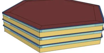
3.4 A building with many different shape factors
To assess the predictive performance of LRBEM+ for a building with multiple changes simultaneously affecting the energy loads, a building that constitutes all the changes reflected by Cases A, B, C, and D (described in the previous section) was designed as Case E (Figure 3.10). It includes the self-shading effect due to the presence of a courtyard. Non-uniform roof heights are incorporated by having 58.6% of the first floor area cover by roof, in addition to the roof on the top floor. This building also includes varying floor heights; the first floor height is 17 ft, while the other floors are 15 ft high. The shape of the building was changed by including on the first floor two right-angled corners, two corners at 102.9°, and another at 154.2°.
The performance of LRBEM+ was evaluated in terms of the predicted change in heating and cooling loads in comparison to that simulated by EnergyPlus associated with a change in the value of a single explanatory variable. For example, the change is heating energy load was predicted using LRBEM+ when one building parameter is incremented from a baseline value. The increase from the baseline set of values for each parameter was set to 25% of the Monte Carlo simulation ranges presented in Table 2.1. Table 3.2 lists the building parameters that were changed, and the corresponding baseline and incremented values for each parameter. This evaluation was conducted for each climate zone.
Table 3.2: Building parameter values for the baseline and the increased value of each building parameter used to test the LRBEM+ energy prediction for Case E.
Baseline 25% Increase on Monte Carlo range
Building Floor Area (m2) 3,724 5,574
Orientation (degrees) 0 45.0
Roof Emissivity 0.90 0.923
Roof Solar Absorptance 0.70 0.895
Roof R-Value 25.8 34.6
Window SHGC (N,S,E,W) 0.35 0.45
Window R-Value (N,S,E,W) 2.22 3.02
Wall R-Value (N,S,E,W) 18.3 26.3
Shading Projection Factor (N,S,E,W) 0.50 0.738
Window-to-Wall Ratio (N,S,E,W) 40% 62%
The baseline energy load for Winston-Salem predicted by LRBEM+ and
71.05 MWh, respectively, for cooling. Figure 3.12 shows the relative change in energy loads in response to the change in each parameter for the Case E building (shown in Figure 3.9). This bar chart compares the LRBEM+ predictions of energy load changes for the Winston-Salem case with EnergyPlus simulated changes. Similar comparisons were conducted for the other climate zones, and the results are presented in Figure 3.11, Figure 3.13, and Figure 3.14.
Figure 3.11: Comparison of relative change is cooling and heating energy loads (for Miami) predicted by LRBEM+ (red) and EnergyPlus (blue) in response to incremental change in each building parameter (Table 7). Parameters on x-axis are ranked by level of importance (left being most influential).
-0.3 -0.2 -0.1 0 0.1 0.2 0.3 0.4 0.5 Fl o o r A re a N o rt h W /W So ut h W /W W es t W /W So ut h W ind o w R -V al ue O ri en tat io n ( d eg re es ) W es t W ind o w R -Val ue Ea st W /W N o rt h W ind o w R -Val ue Ea st W in d o w R -Va lu e R o o f R -V al ue So ut h SH G C W es t SH G C R o o f Em is si vi ty Ea st SH G C R o o f So lar Abs o rpt an ce N o rt h SH G C W es t W al l R -Va lu e Ea st W al l R -Val ue Ea st SP F N o rt h SP F So u th SP F N o rt h W al l R -Val u e W es t SP F So ut hWa ll R -Va lue M wh E n e rg y Ch an
ge Cooling in Miami
Simulation Prediction -100 10 20 30 40 50 60 70 80 Fl o o r A re a N o rt h W /W So ut h W /W Ea st W /W So ut h SP F So ut h SH G C N o rt h SH G C Ea st SH G C N o rt h SP F W es t W /W W es t SH G C Ea st SP F R o o f So lar Abs o rpt an ce W es t SP F R o o f Em is si vi ty W es t W al l R -Val ue R o o f R -V al ue N o rt h W ind o w R -Val ue So ut h W ind o w R -V al ue Ea st W ind o w R -Val ue W es t W ind o w R -Val ue Ea st W al l R -Val ue So ut hWa ll R -Va lue N o rt h W al l R -Val u e O ri ent at io n (de gr ee s) M B TU E n e rg y Ch an ge
Heating in Miami
Figure 3.12: Comparison of relative change is cooling and heating energy loads (for Winston-Salem) predicted by LRBEM+ (red) and EnergyPlus (blue) in response to the incremental change in each building parameter (Table 7). Parameters on x-axis are ranked by level of importance (left being most influential).
-10 -5 0 5 10 15 20 25 30 35 Fl o o r A re a O ri ent at io n (de gr ee s) W ind o w S H G C S o ut h Sha di ng P ro je ct io n Fac to r… W ind o w S H G C N o rt h W ind o w-to -W al l R at io S o ut h Sha di ng P ro je ct io n Fac to r… W ind o w-to -W al l R at io N o rt h W ind o w S H G C East W ind o w-to -W al l R at io E as t W ind o w-to -W al l R at io W est W ind o w S H G C W est Sha di ng P ro je ct io n Fac to r East R o o f So lar Abs o rpt an ce Sha di ng P ro je ct io n Fac to r… R o o f Em is si vi ty W ind o w R -Val ue N o rt h W ind o w R -Val ue S o ut h R o o f R -V al ue W ind o w R -Val ue E as t W ind o w R -Val ue W est W al l R -V al ue E as t W al l R -V al ue N o rt h W al l R -V al ue W est W al l R -V al ue S o ut h M wh E n e rg y Ch an
ge Cooling in Winston-Salem
Prediction Simulation -20 -10 0 10 20 30 40 Fl o o r A re a W ind o w-to -W al l R at io S o ut h W ind o w-to -W al l R at io N o rt h W ind o w-to -W al l R at io W est W in d o w R -Va lu e N o rt h W ind o w R -Val ue S o ut h W ind o w R -Val ue W est W ind o w-to -W al l R at io E as t O ri ent at io n (de gr ee s) R o o f R -V al ue W ind o w R -Val ue E as t W ind o w S H G C N o rt h W ind o w S H G C S o ut h W al l R -V al ue W est W ind o w S H G C East W in d o w SHG C W es t Sha di ng P ro je ct io n Fac to r… Sha di ng P ro je ct io n Fac to r… R o o f So lar Abs o rpt an ce Sha di ng P ro je ct io n Fac to r East R o o f Em iss iv it y Sha di ng P ro je ct io n Fac to r… W al l R -V al ue S o ut h W al l R -V al ue N o rt h M B TU E n e rg y Ch an
ge Heating in Winston-Salem
Figure 3.13: Comparison of relative change is heating energy load (for Albuquerque) predicted by LRBEM+ (red) and EnergyPlus (blue) in response to incremental change in each building parameter (Table 7). Parameters on x-axis are ranked by level of importance (left being most influential).
-40 -30 -20 -10 0 10 20 30 40 50
M
wh
E
n
e
rg
y
Ch
an
ge
Cooling in Albuquerque
Simulation Prediction
-5 0 5 10 15 20 25 30
M
B
TU
E
n
e
rg
y
Ch
an
ge
Heating in Albuquerque
Figure 3.14: Comparison of relative change is heating energy load (for Minneapolis) predicted by LRBEM+ (red) and EnergyPlus (blue) in response to incremental change in each building parameter (Table 7). Parameters on x-axis are ranked by level of importance (left being most influential).
-5 0 5 10 15 20 25 M wh E n e rg y Ch an ge
Cooling in Minneapolis
Simulation Prediction -100 -50 0 50 100 150 200 250 300 350 Fl o o r A rea So u th W /W N o rt h W /W W es t W /W Ea st W /W N o rt h W in d o w R -Va lu e So u th W in d o w R -V al u e W es t W in d o w R -Va lu e R o o f R -Va lu e Ea st W in d o w R -Va lu e W es t W al l R -Va lu e So u th S H G C N o rt h S HG C Ea st S HG C O ri en ta ti o n ( d e gr ee s) So u th S P F W es t SH G C N o rt h S PF Ea st S PF R o o f E m is si vi ty R o o f S o la r A b so rp ta n ce W es t SPF N o rt h W al l R -Va lu e So u th W al l R -Va lu e Ea st W al l R -V al u e M B TU E n e rg y Ch an ge
Heating in Minneapolis
Chapter 4
Outcome and Discussion
Rapid feedback on building energy performance during the early design stages can help guide sustainable and efficient building design. Existing building energy simulation models require detailed building specifications and are complex to operate. Such models are of little value during the early design stages when architects are experimenting with massing, orientation, and fenestration. In previous work, a linear regression-based building energy model (LRBEM) was developed by iterating EnergyPlus within a Monte Carlo framework (Hygh et al, 2012). While LRBEM provided rapid and accurate estimates of heating and cooling loads, it was limited to rectangular, medium-sized office buildings.
The work presented in this thesis represents a significant extension of LRBEM by generalizing the prediction capability to medium-sized commercial buildings with any arbitrary geometry. The updated model, referred to as LRBEM+, represents a revised multivariate linear regression equation based on 30 early building design parameters using results from the original 20,000 Monte Carlo realizations. The new model, LRBEM+, can accurately predict the heating and cooling loads associated with complex building
LRBEM+ could serve as a practical substitute for building energy simulation engines in early building design stages by providing instantaneous feedback on energy performance through the specification of a limited number of early design parameters. Like LRBEM, the new model LRBEM+ is currently limited to four climate zones in the United States
represented by the cities Winston-Salem, Miami, Albuquerque, and Minneapolis, which are meant to span the climatic extremes within the continental U.S. Future work could extend LRBEM+ development beyond these four climate zones. In addition, the model could be extended to predict different building categories, such as large and small sized office
buildings, hotels, high and low raise residential, warehouses, malls, and retail stores. Another extension would be the application of formal search techniques to help identify optimal design solutions. Such solutions could be reached by allowing users to optimize a subset of their design decisions to minimize heating and cooling loads. Availability of LRBEM+ is significant because it can serve as a practical decision support tool for architects during the early design stages, where building design decisions have strong implications on realized energy performance yet tools to assess energy are most lacking. By targeting the early design phase, the intention of LRBEM+ is to transform the perception of building energy
REFERENCES
(ASHRAE), A. S. (2007). Energy Standard for. Buildings Except. Low-Rise Residential.
Atlanta, GA: ASHRAE.
American Institute of Architects. (2012). An Architects Guide to intergrating energy
modeling in the deisgn process. U.S.A: AIA.
Deru M, F. K. (2011). US Department of Energy commercial reference building models of
the National Stock. National Renewable Energy Laboratory.
Hygh, J. S. (2011). Implementing Energy Simulation as a Design Tool in Conceptual
Building Design with. Raleigh, NC: North Carolina State University.
Hygh, J. S., DeCarolis, J., B.Hill, D., & Ranjithan, R. (2012). Multivariate Regression as an energy assessment tool in early building design. Building and Environment, 165-175. Maile, T., Fischer, M., & Bazjanac, V. (2007). Building Energy Performance Simulation
Tool- a Life cycle and Interoperable Perspective. Standford University.
Mathworks. (2013). Documentation Center- Stepwisefit. Retrieved 2013, from Statistical tool box, Linear Regresson: http://www.mathworks.com/help/stats/stepwisefit.html
Urban, B., & Glicksman., L. (Dec 2007). A rapid building energy model and interface for non-technical users." Proceedings of the 10th ORNL Thermal Performance of the
Exterior Envelopes of Whole Buildings International Conference. Clearwater, FL:
MIT.
US EnergyInformation Administration. (2010). International Energy Statistics. Retrieved 2013, from US EnergyInformation Administration:
http://www.eia.gov/cfapps/ipdbproject/IEDIndex3.cfm?tid=44&pid=44&aid=2 Yale University. (2012). Multiple Linear Regression. Retrieved 2013, from Statistics At
Appendix I
Figure 5.1: Framework of method “combination of rectangles”.
Appendix II
Figure 5.2: Framework of method “Perimeter Preserved”.
Appendix III
Figure 5.3: The framework for “Floor Area Preserved”.
Appendix IV
Figure 5.4: the Framework for “Bigger Rectangular with Area Factor”.
Appendix V
Table 5.1: Final cross product parameters, as well as their values that were included in the heating equation for the LRBEM+.
1A- Miami
4A- Winston-Salem
4B-Albuquerq ue
6A-
Minneapol is
4.99E+08 3.84E+09 2.85E+09 5.69E+10 Intercept -2.17E+05 -9.35E+06 -1.24E+07 -1.73E+07 Area in m2 -1.75E+05 3.19E+07 3.37E+07 1.98E+08 Wall A w -4.65E+05 2.46E+07 2.17E+07 1.85E+08 Wall A S -1.75E+05 3.19E+07 3.37E+07 1.98E+08 Wall A E -4.65E+05 2.46E+07 2.17E+07 1.85E+08 Wall A N
-7.76E+08 -1.39E+11 -1.72E+11 -4.89E+11 Wall U-Value West -9.08E+07 -5.03E+09 -6.56E+09 4.77E+09 Wall U-Value South -7.78E+07 5.98E+08 2.30E+09 -1.26E+09 Wall U-Value East -2.89E+07 1.17E+09 6.84E+08 6.76E+09 Wall U-Value North
-1.19E+08 -3.23E+09 -5.29E+09 -1.38E+10 Window-to-Wall Ratio West -1.21E+09 5.48E+09 2.68E+09 2.23E+10 Window-to-Wall Ratio South 1.90E+07 -1.64E+10 -2.52E+10 -5.66E+10 Window-to-Wall Ratio East -1.03E+09 -6.02E+09 -1.49E+10 -1.05E+10 Window-to-Wall Ratio North -3.30E+05 1.84E+07 3.44E+07 2.18E+07 window Area West
1.17E+06 3.50E+07 6.08E+07 5.91E+07 Window Area South 1.81E+05 5.55E+07 8.16E+07 1.64E+08 Window Area East 8.18E+05 4.22E+07 6.82E+07 8.30E+07 Window Area North
1.23E+06 6.28E+07 7.75E+07 2.42E+08 West Win U-value * Window Area
8.80E+05 6.02E+07 7.54E+07 2.22E+08 South U-value * Window Area 6.88E+05 5.58E+07 6.66E+07 2.14E+08 East U-value * Window Area 7.65E+05 6.26E+07 7.75E+07 2.21E+08 North U-value * Window Area 9.39E+05 4.31E+07 5.43E+07 1.45E+08 Roof Emissivity * Roof
Area/number of stories
-1.42E+05 -7.27E+06 -1.07E+07 -1.35E+07 Roof Solar Absorptance * Roof Area
Continue Table 5.1
-2.96E+06 -2.25E+08 -3.34E+08 -6.10E+08 South SHGC * Window Area -2.31E+06 -2.51E+08 -3.53E+08 -6.33E+08 East SHGC * Window Area -8.34E+05 -2.22E+08 -3.17E+08 -5.94E+08 North SHGC * Window Area 2.06E+07 7.44E+09 1.03E+10 2.28E+10 West Shading Project Factor *
window-to-wall ratio
1.01E+08 3.67E+10 5.44E+10 1.24E+11 South Shading Project Factor * window-to-wall ratio
1.07E+08 2.50E+10 3.84E+10 7.56E+10 East Shading Project Factor * window-to-wall ratio
9.87E+07 3.24E+10 4.66E+10 1.11E+11 North Shading Project Factor * window-to-wall ratio
1.91E+08 8.78E+09 1.69E+10 4.81E+09 sin(orientation)+abs(cos(orientati on))
1.28E+05 1.06E+07 1.78E+07 6.57E+06 West U-value * Window Area * sin(O)+abs(cos(O))
8.81E+04 3.12E+06 5.11E+06 -1.35E+06 South U-value * Window Area * sin(O)+abs(cos(O))
5.41E+04 -3.01E+06 -4.86E+06 -7.42E+05 East U-value * Window Area * sin(O)+abs(cos(O))
4.72E+04 8.19E+05 7.83E+05 -1.42E+05 North U-value * Window Area * sin(O)+abs(cos(O))
9.05E+05 -1.15E+08 -1.55E+08 -4.52E+08 West Wall U-value * Opaque Wall Area
7.48E+04 -6.35E+06 -7.17E+06 -2.75E+07 South Wall U-value * Opaque Wall Area
-3.97E+05 -2.12E+06 -6.96E+05 -2.43E+06 East Wall U-value * Opaque Wall Area
-5.67E+04 1.71E+06 1.57E+06 1.03E+07 North Wall U-value * Opaque Wall Area
3.63E+05 1.01E+08 1.59E+08 4.01E+08 West SHGC * Window Area * sin(O)+abs(cos(O))
5.51E+05 8.35E+06 1.59E+07 8.93E+05 South SHGC * Window Area * sin(O)+abs(cos(O))
3.63E+05 -3.43E+07 -5.08E+07 -1.15E+08 East SHGC * Window Area * sin(O)+abs(cos(O))
Table 5.2: Final cross product parameters, as well as their values that were included in the cooling equation for the LRBEM+.
1A- Miami
4A- Winston-Salem
4B-Albuquerq ue
6A-
Minneapol is
-2.71E+10 -1.38E+10 -2.38E+10 -1.49E+10 intercept 1.38E+08 8.57E+07 6.88E+07 5.46E+07 Area in m2 4.76E+07 -4.89E+06 -9.00E+06 -6.57E+06 Wall A w 3.94E+07 -8.77E+06 -1.40E+07 -9.46E+06 Wall A S 4.76E+07 -4.89E+06 -9.00E+06 -6.57E+06 Wall A E 3.94E+07 -8.77E+06 -1.40E+07 -9.46E+06 Wall A N
2.53E+10 1.96E+10 2.13E+10 1.50E+10 Window-to-Wall Ratio West 8.52E+10 5.70E+10 6.28E+10 4.39E+10 Window-to-Wall Ratio South 4.22E+10 3.66E+10 4.18E+10 2.64E+10 Window-to-Wall Ratio East 9.70E+10 6.26E+10 7.89E+10 4.61E+10 Window-to-Wall Ratio North -6.63E+07 -3.83E+07 -3.73E+07 -2.61E+07 window Area West
-6.33E+07 -4.99E+07 -5.14E+07 -3.22E+07 Window Area South -5.82E+07 -6.34E+07 -6.73E+07 -3.78E+07 Window Area East -7.35E+07 -5.66E+07 -6.51E+07 -3.69E+07 Window Area North
3.58E+06 -7.15E+06 -5.80E+06 -5.67E+06 West Win U-value * Window Area
4.63E+06 -7.58E+06 -7.35E+06 -6.45E+06 South U-value * Window Area 6.07E+06 -7.80E+06 -8.14E+06 -6.65E+06 East U-value * Window Area 5.17E+06 -7.54E+06 -7.09E+06 -5.91E+06 North U-value * Window Area -5.44E+07 -5.93E+07 -6.20E+07 -4.20E+07 Roof Emissivity * Roof Area 1.54E+07 1.38E+07 1.46E+07 7.71E+06 Roof Solar Absorptance * Roof
Area
-1.31E+07 1.01E+07 7.52E+06 6.68E+06 Roof R-value * Roof Area 5.77E+08 4.16E+08 4.62E+08 2.83E+08 West SHGC * Window Area 4.44E+08 3.22E+08 3.34E+08 2.29E+08 South SHGC * Window Area 4.25E+08 3.11E+08 3.49E+08 2.22E+08 East SHGC * Window Area 4.46E+08 3.20E+08 4.26E+08 2.32E+08 North SHGC * Window Area -3.98E+10 -2.70E+10 -3.00E+10 -2.08E+10 West Shading Project Factor *
window-to-wall ratio
-1.49E+11 -1.20E+11 -1.30E+11 -8.98E+10 South Shading Project Factor * window-to-wall ratio
Continue Table 5.2
-1.36E+11 -1.03E+11 -1.26E+11 -7.61E+10 North Shading Project Factor * window-to-wall ratio
-8.29E+08 -1.78E+09 -2.12E+09 -8.41E+07 sin(orientation)
4.09E+10 2.57E+10 4.26E+10 2.93E+10 sin(orientation) squared -1.30E+08 1.52E+07 2.46E+06 1.28E+07 West Wall U-value * Opaque
Wall Area
1.02E+06 3.24E+06 2.61E+06 1.21E+06 South Wall U-value * Opaque Wall Area
2.21E+06 7.45E+05 2.18E+06 2.28E+06 East Wall U-value * Opaque Wall Area
4.65E+05 -2.18E+06 -9.77E+05 -7.65E+05 North Wall U-value * Opaque Wall Area
-1.45E+08 -1.27E+08 -1.37E+08 -6.35E+07 West SHGC * Window Area * sin(O)+abs(cos(O))
3.42E+07 4.27E+07 6.53E+07 3.53E+07 South SHGC * Window Area * sin(O)+abs(cos(O))
9.38E+07 9.85E+07 1.34E+08 6.35E+07 East SHGC * Window Area * sin(O)+abs(cos(O))
Table 5.3: List of building parameters and derived parameters that went into the Stepwise Regression.
Building Parameter Terms
1 Area in m2
2 Wall A w
2 Wall A S
4 Wall A E
5 Wall A N
6 Surface Area
7 Orientation
8 Roof Emissivity
9 Roof Solar Absorptance
10 Roof R-Value
11 Window SHGC West
12 Window SHGC South
13 Window SHGC East
14 Window SHGC North
15 Window U-Value West
16 Window U-Value South
17 Window U-Value East
18 Window U-Value North
19 Wall U-Value West
20 Wall U-Value South
21 Wall U-Value East
22 Wall U-Value North
23 Shading Projection West
24 Shading Projection South
25 Shading Projection East
26 Shading Projection North
27 Window-to-Wall Ratio West
28 Window-to-Wall Ratio South
29 Window-to-Wall Ratio East
Continue Table 5.3
Derived Parameters- Cross Multiplied Terms
31 Window Area West
32 Window Area South
32 Window Area East
34 Window Area North
35 West Window Area * cos(rotation) 36 South Window Area * cos(rotation) 37 East Window Area * cos(rotation) 38 North Window Area * cos(rotation) 39 West Win U-value * Window Area
40 South U-value * Window Area
41 East U-value * Window Area
42 North U-value * Window Area
43 Roof Emissivity * Roof Area
44 Roof Solar Absorptance * Roof Area
45 Roof R-value * Roof Area
46 Roof Emissivity * Roof Area / Number of Stories
47 Roof Solar Absorptance * Roof Area / Number of Stories 48 Roof R-value * Roof Area / Number of Stories
49 West SHGC * Window Area
50 South SHGC * Window Area
51 East SHGC * Window Area
52 North SHGC * Window Area
53 West Shading Project Factor * window-to-wall ratio 54 South Shading Project Factor * window-to-wall ratio 55 East Shading Project Factor * window-to-wall ratio 56 North Shading Project Factor * window-to-wall ratio
57 north window area^2
58 south window area^2
59 sin(orientation)
60 cos(orientation)
61 abs(cos(orientation))
Continue Table 5.3
63 cos(orientation) squared
64 sin(orientation)+abs(cos(orientation))
65 West U-value * Window Area * sin(O)+abs(cos(O)) 66 South U-value * Window Area * sin(O)+abs(cos(O)) 67 East U-value * Window Area * sin(O)+abs(cos(O)) 68 North U-value * Window Area * sin(O)+abs(cos(O)) 69 3-[sin(orientation) + abs(cos(orientation))]
70 West Window Area * [sin(O) + abs(cos(O))] 71 South Window Area * [sin(O) + abs(cos(O))] 72 East Window Area * [sin(O) + abs(cos(O))] 73 North Window Area * [sin(O) + abs(cos(O))] 74 West Wall U-value * Opaque Wall Area 75 South Wall U-value * Opaque Wall Area 76 East Wall U-value * Opaque Wall Area 77 North Wall U-value * Opaque Wall Area
78 West SHGC * Window Area * sin(O)+abs(cos(O)) 79 South SHGC * Window Area * sin(O)+abs(cos(O)) 80 East SHGC * Window Area * sin(O)+abs(cos(O)) 81 North SHGC * Window Area * sin(O)+abs(cos(O)) 82 West Shading Project Factor * window-to-wall ratio *
sin(O)+abs(cos(O))
83 South Shading Project Factor * window-to-wall ratio * sin(O)+abs(cos(O))
84 East Shading Project Factor * window-to-wall ratio * sin(O)+abs(cos(O))
85 North Shading Project Factor * window-to-wall ratio * sin(O)+abs(cos(O))
86 Roof Area
Table 5.4: Building in Figure 3.1 parameter definitions.
Parameter Value
Total Floor Area 8926 (m2)
Envelop Area/ Floor Area 0.89
Orientation 0
Stories 3
Window/Wall ratio (N,S, E,W) 40%
Shading Projection Factor (N,S, E,W) 0.5
Window SHGC (N,S, E,W) 0.35
Window R Value (N,S, E,W) 2.22
Wall R Value (N,S, E,W) 18.3
Roof Emissivity 0.9
Roof Solar Absorptance 0.7
Roof R Value 25.8
Table 5.5: Experiments A through C parameter definitions. R Values are in
(BTU/hft^2f), Areas in Meter
A1 A2 B1 B2 C1 C2 Units
Building Floor Area 5,775 5,217 2,174 6,53 5
7,2 23
9,7 51
M²
Roof Area 1,925 1,739 725 2,17
8
3,3 13
4,5 79
M²
Orientation - - - Degrees
West Wall Area 617 672 334 397 962 1,1 65
M² South Wall Area 891 1,083 591 794 481 1,0
97 M² East Wall Area 617 672 - 397 962 1,1
65 M² North Wall Area 891 1,083 591 794 481 1,0
97 M² Roof Emissivity 0.9 0.9 0.9 0.9 0.9 0.9 - Roof Solar Absorptance 0.7 0.7 0.7 0.7 0.7 0.7 - Roof R-Value 25.8 25.8 25.8 25.8 25.
8
25. 8
Continue table 5.5
West Window SHGC 0.35 0.35 0.35 0.35 0.3 5
0.3 5
- South Window SHGC 0.35 0.35 0.35 0.35 0.3
5
0.3 5
- East Window SHGC 0.35 0.35 0.35 0.35 0.3
5
0.3 5
- North Window SHGC 0.35 0.35 0.35 0.35 0.3
5
0.3 5
- West Window R-Value 2.22 2.22 2.22 2.22 2.2
2
2.2 2
(BTU/hf t^2f) South Window R-Value 2.22 2.22 2.22 2.22 2.2
2
2.2 2
(BTU/hf t^2f) East Window R-Value 2.22 2.22 2.22 2.22 2.2
2
2.2 2
(BTU/hf t^2f) North Window R-Value 2.22 2.22 2.22 2.22 2.2
2
2.2 2
(BTU/hf t^2f) West Wall R-Value 18.30 18.30 18.30 18.3
0 18. 30 18. 30 (BTU/hf t^2f) South Wall R-Value 18.30 18.30 18.30 18.3
0 18. 30 18. 30 (BTU/hf t^2f) East Wall R-Value 18.30 18.30 18.30 18.3
0 18. 30 18. 30 (BTU/hf t^2f) North Wall R-Value 18.30 18.30 18.30 18.3
0 18. 30 18. 30 (BTU/hf t^2f) West Shading Projection
Factor
0.500 0.500 0.500 0.50 0 0.5 00 0.5 00 % of window height Shading Projection Factor
South
0.500 0.500 0.500 0.50 0 0.5 00 0.5 00 % of window height East Shading Projection
Factor
0.500 0.500 0.500 0.50 0 0.5 00 0.5 00 % of window height North Shading Projection
Factor
0.500 0.500 0.500 0.50 0 0.5 00 0.5 00 % of window height West Window-to-Wall Ratio
Continue Table 5.5 South Window-to-Wall Ratio
40.00% 40.00 % 40.00 % 40.0 0% 40. 00 % 40. 00 % % East Window-to-Wall Ratio
40.00% 40.00 % 40.00 % 40.0 0% 40. 00 % 40. 00 % % North Window-to-Wall Ratio
40.00% 40.00 % 40.00 % 40.0 0% 40. 00 % 40. 00 % %
Table 5.6: Ranking of the 30 parameters according to their importance in heating in the four climate zones, knowing that the importance of wall, roof, floor areas are
aggregated with parameter term areas.
Miami Winston-Salem Albuquerque Minneapolis
Areas Areas South W/W Areas
North W/W
Window-to-Wall Ratio
South Areas South W/W
South W/W
Window-to-Wall Ratio
North North W/W North W/W
West W/W
Window-to-Wall Ratio
West West W/W West W/W
South Window R-Value
Window R-Value North
South Window
R-Value East W/W
Orientation (degrees)
Window R-Value South
East Window R-Value
North Window R-Value West Window
R-Value Window R-Value West
North Window R-Value South Window R-Value East W/W Window-to-Wall Ratio East Orientation (degrees) West Window R-Value North Window
R-Value Orientation (degrees)
West Window
R-Value Roof R-Value
East Window
R-Value Roof R-Value East W/W
East Window R-Value
Roof R-Value Window R-Value East South SHGC
West Wall R-Value
Continue Table 5.6
Roof Emissivity Wall R-Value West West Wall R-Value East SHGC East SHGC Window SHGC East East SHGC
Orientation (degrees) Roof Solar
Absorptance Window SHGC West West SHGC South SPF North SHGC
Shading Projection
Factor South South SPF West SHGC
West Wall R-Value
Shading Projection
Factor North North SPF North SPF
East Wall R-Value
Roof Solar
Absorptance East SPF East SPF
East SPF
Shading Projection Factor East
Roof Solar
Absorptance Roof Emissivity North SPF Roof Emissivity Roof Emissivity
Roof Solar Absorptance South SPF
Shading Projection
Factor West West SPF West SPF
North Wall
R-Value Wall R-Value South SouthWall R-Value
North Wall R-Value
West SPF Wall R-Value North East Wall R-Value
SouthWall R-Value
SouthWall
R-Value Wall R-Value East North Wall R-Value
Table 5.7: Ranking of the 30 parameters according to their importance in cooling in the four climate zones, knowing that the importance of wall, roof, floor Areas are
aggregated with Areas.
Miami Winston-Salem Albuquerque Minneapolis
Areas Areas Areas Areas
North W/W Orientation (degrees)
Orientation (degrees)
Orientation (degrees) South W/W Window SHGC South North W/W South SHGC East W/W
Shading Projection
Factor South North SHGC South SPF South SPF Window SHGC North South SHGC North SHGC South SHGC
Window-to-Wall Ratio
South South SPF South W/W
North SHGC
Shading Projection
Factor North South W/W North SPF
East SHGC
Window-to-Wall Ratio
North North SPF North W/W
North SPF Window SHGC East East SHGC East SHGC West W/W
Window-to-Wall Ratio
East East W/W West W/W
West SHGC
Window-to-Wall Ratio
West West W/W East W/W
East SPF Window SHGC West East SPF West SHGC
Roof Solar Absorptance
Shading Projection
Factor East West SHGC East SPF
West SPF Roof Solar Absorptance Roof Solar Absorptance Roof Solar Absorptance Roof Emissivity Shading Projection
Factor West West SPF West SPF
West Wall
R-Value Roof Emissivity Roof Emissivity Roof Emissivity Roof R-Value
Window R-Value North
South Window R-Value
South Window R-Value
North Window R-Value
Window R-Value South
North Window R-Value
North Window R-Value
South Window
R-Value Roof R-Value
East Window R-Value
East Window R-Value
East Window
Continue Table 5.7 West Window R-Value
Window R-Value West
West Window R-Value
West Window R-Value
East Wall R-Value Wall R-Value East West Wall R-Value West Wall R-Value South Wall R-Value Wall R-Value North East Wall R-Value East Wall R-Value North Wall R-Value Wall R-Value West North Wall R-Value South Wall R-Value Orientation