Multivariate GARCH Modeling and Comparison to Real Kernel Estimates.

ABSTRACT

YU, YANRU. Multivariate GARCH Modeling and Comparison to Real Kernel Estimates. (Under the direction of Professor Denis Pelletier and Professor Doug Pearce).

In this dissertation we make two contributions to the current multivariate volatility literature. Firstly, we provide an original approach for comparing the relative performance of existing multivariate GARCH models. These models produce forecasts for quantities that cannot be directly observed: variances, covariances, and correlations. From the recent literature on realized volatility, we now have very precise measurements of these objects that can be computed with so called intra-day high-frequency data. We called them realized variance, covariance, and correlation. We can use them as a target against which we can now compare the accuracy of the forecasts generated by the multivariate GARCH models (for the daily returns). In an empirical application, we compare the performance of ten of the most popular multivariate GARCH models in terms of forecasting accuracy and computational time. We find that the DCC model of Engle (2002) is the model that performs best.

Multivariate GARCH Modeling and Comparison to Real Kernel Estimates

by Yanru Yu

A dissertation submitted to the Graduate Faculty of North Carolina State University

in partial fulfillment of the requirements for the degree of

Doctor of Philosophy

Economics

Raleigh, North Carolina 2012

APPROVED BY:

_______________________________ ______________________________

Dr. Doug Pearce Dr. Denis Pelletier

Committee Co-Chair Committee Co-Chair

________________________________ ________________________________

ii DEDICATION

To My Daughter Stacy Peng and my husband

Yuantao Peng And my parents

iii BIOGRAPHY

iv ACKNOWLEDGMENTS

It is a long journey, for me, for my advisor and for the family. I thank my advisor Dr. Denis Pelletier for his priceless advice and his relentless effort to guide me to where I am today. I give my gratitude to all the committee members for their precious opinions on the

v TABLE OF CONTENTS

List of Tables ... vii

List of Figures ... viii

Introduction ... 1

Chapter 1 Review of GARCH Modeling and Realized Volatility Literature ... 7

1.1 Introduction ... 7

1.2 The Realized Volatility ... 8

1.3 The Real Kernel Model ... 17

1.4 The Multivariate Real Kernel Estimator ... 26

1.5 The Multivariate GARCH (MGARCH) models ... 30

1.6 Conclusion ... 41

Chapter 2 Data Analysis of the MGARCH Models Comparison ... 43

2.1 Introduction ... 44

2.1.1 Data Description ... 44

2.1.2 The Real Kernel Estimate ... 45

2.2 The MGARCH Models Estimation ... 47

2.2.1 The Diagonal VEC model ... 48

2.2.2 The BEKK(1,1,1) model ... 55

2.2.3 The Factor-GARCH(1,1,k) model ... 62

2.2.4 The Full Factor-MGARCH (FF-MGARCH) model ... 68

2.2.5 The Orthogonal-GARCH(1,1,m) model ... 76

2.2.6 The Generalized Orthogonal GARCH (1, 1) model ... 83

2.2.7 The Constant Conditional Correlation (CCC) model ... 90

2.2.8 Dynamic Conditional Correlation (DCC) model by Tse and Tsui ... 91

2.2.9 The Dynamic Conditional Correlation (DCC) model by Engle ... 98

2.2.10 The Regime Switching Dynamic Correlation (RSDC) Model ... 105

2.2.11 Model Comparison... 114

2.3 Conclusion ... 117

Chapter 3 The Real Dynamic Conditional Correlation Model ... 119

3.1 Introduction ... 119

vii LIST OF TABLES

Table 2.1.1- 1 List of the stocks for the model comparison ... 45

Table 2.2.1-1 Distance of the correlations by the DVEC model ... 49

Table2.2.1- 2 The parameter estimates of the DVEC model ... 51

Table 2.2.2- 1 Distance of the correlations by the BEKK(1,1,1) model... 55

Table 2.2.2- 2 The parameter estimates of the BEKK(1,1,1) model ... 57

Table 2.2.3- 1 Distance of the correlations by the FGARCH(1,1,1) model ... 64

Table 2.2.3- 2 The Parameter Estimates of the FGARCH(1,1,1) model ... 65

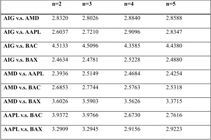
Table 2.2.4- 1 Distance of the correlations by the FFGARCH model ... 69

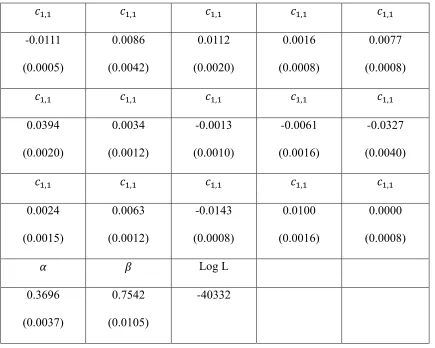
Table 2.2.4- 2 The parameter Estimates of the Full Factor GARCH model ... 70

Table 2.2.5- 1 Distance of the correlations by the O-GARCH(1,1,n) model ... 77

Table 2.2.5- 2 The parameter estimates of the O-GARCH(1,1,n) model ... 78

Table 2.2.6- 1 Distance of the correlations by the GO-GARCH model ... 84

Table 2.2.6- 2 The parameter estimates of the GO-GARCH model ... 85

Table 2.2.8- 1 Distance of the correlations by the DCC Tse and Tsui model ... 92

Table 2.2.8- 2 The Parameter Estimates of the individual GARCH processes ... 93

Table 2.2.8- 3 The Parameter Estimates of the Correlation Equation ... 94

Table 2.2.9- 1 Correlations by DCC Engle ... 99

Table 2.2.9- 2 The Parameter Estimates of the individual GARCH processes ... 101

Table 2.2.9- 3 The parameter estimates of the correaltion equation ... 101

Table 2.2.10- 1 Distance of the correlations by the RSDC model ... 106

Table 2.2.10- 2 The parameter estimates of the RSDC model ... 107

Table 2.2.11- 1 Model Comparison: distance to the real kernel estimates ... 115

Table 2.2.11- 2 Model Comparison: Computation time ... 116

Table 3.3- 1 The parameter estimates for the real GARCH model ... 129

Table 3.3- 2 The parameter estimates for the real DCC model ... 130

Table 3.3- 3 Distance comparison of the real GARCH and the GARCH(1,1) model ... 132

Table 3.3- 4 The computation time of the real GARCH and the GARCH(1,1) models ... 132

Table 3.3- 5 Distance Comparison for the case n=2 ... 134

Table 3.3- 6 Computation Time Comparison for the case n=2 (in seconds) ... 135

Table 3.3- 7 Distance Comparison For the case n=3 ... 137

Table 3.3- 8 Computation Time Comparison for the case n=3... 137

Table 3.3- 9 Distance Comparison for the case that n=4 ... 138

Table 3.3- 10 Computation Time Comparison for the case that n=4 ... 138

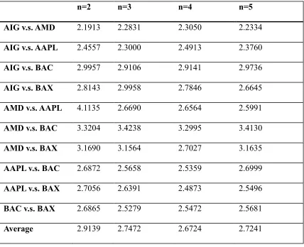
Table 3.3- 11 Distance Comparison for the case that n=5 ... 139

Table 3.3- 12 Computation Time Comparison for the case that n=5 ... 139

Table 3.3- 13 Distance between the forecasted correlations by the real DCC model to the real kernel estimates of the actual correlations ... 141

Table 3.3- 14 Distance of the correlations from the DCC-X model ... 146

viii LIST OF FIGURES

Figure 1. 1 Average (across days) value of the RV drawn against M. ... 15 Figure 1.4- 1 Multivariate real kernel data series alignment ... 28 Figure 2.1.2- 1 Real kernel estimates of correlation between AIG and BAC in different dimensions. Time Period: All the trading days from Jan 1st, 2003 to Dec 31st, 2003. ... 46 Figure 2.1.2- 2 Real kernel estimates of correlation between BAC and BAX in different dimensions. Time Period: All the trading days from Jan 1st, 2003 to Dec 31st, 2003. ... 47 Figure 2.1.2- 3 Real kernel estimates of correlation between AMD and AAPL in different dimensions. Time Period: All the trading days from Jan 1st, 2003 to Dec 31st, 2003. ... 47 Figure 2.2.1- 1 The contrast plot of the correlation between AIG and BAC by the DVEC model and the real kernel estimate in the case that n=2. Time Period: All the trading days from Jan 1st, 2003 to Dec 31st, 2003... 52 Figure 2.2.1- 2 The contrast plot of the correlation between AIG and BAC by the DVEC model and the real kernel estimate in the case that n=5. Time Period: All the trading days from Jan 1st, 2003 to Dec 31st, 2003... 52 Figure 2.2.1- 3 The contrast plot of the correlation between BAC and BAX by the DVEC model and the real kernel estimate in the case that n=2. Time Period: All the trading days from Jan 1st, 2003 to Dec 31st, 2003... 53 Figure 2.2.1- 4 The contrast plot of the correlation between BAC and BAX by the DVEC model and the real kernel estimate in the case that n=5. Time Period: All the trading days from Jan 1st, 2003 to Dec 31st, 2003... 54 Figure 2.2.1- 5 The contrast plot of the correlation between AMD and AAPL by the DVEC model and the real kernel estimate in the case that n=2. Time Period: All the trading days from Jan 1st, 2003 to Dec 31st, 2003... 54 Figure 2.2.1- 6 The contrast plot of the correlation between AMD and AAPL by the DVEC model and the real kernel estimate in the case that n=5. Time Period: All the trading days from Jan 1st, 2003 to Dec 31st, 2003... 55 Figure 2.2.2- 1 The contrast plot of the correlation between AIG and BAC by the

BEKK(1,1,1) model and the real kernel estimate in the case that n=2. Time Period: All the trading days from Jan 1st, 2003 to Dec 31st, 2003. ... 58 Figure 2.2.2- 2 The contrast plot of the correlation between AIG and BAC by the

BEKK(1,1,1) model and the real kernel estimate in the case that n=5. Time Period: All the trading days from Jan 1st, 2003 to Dec 31st, 2003. ... 59 Figure 2.2.2- 3 The BEKK(1,1,1) estimate of the correlation between AIG and BAC in different dimensions. Time Period: All the trading days from Jan 1st, 2003 to Dec 31st, 2003. ... 59 Figure 2.2.2- 4 The real kernel estimate of the correlation between AIG and BAC in

different dimensions. Time Period: All the trading days from Jan 1st, 2003 to Dec 31st, 2003. ... 60 Figure 2.2.2- 5 The contrast plot of the correlation between BAC and BAX by the

ix Figure 2.2.2- 6 The contrast plot of the correlation between BAC and BAX by the

BEKK(1,1,1) model and the real kernel estimate in the case that n=5. Time Period: All the trading days from Jan 1st, 2003 to Dec 31st, 2003. ... 61 Figure 2.2.2- 7 The BEKK(1,1,1) estimate of the correlation between BAC and BAX in different dimensions. Time Period: All the trading days from Jan 1st, 2003 to Dec 31st, 2003. ... 61 Figure 2.2.2- 8 The real kernel estimate of the correlation between BAC and BAX in

different dimensions. Time Period: All the trading days from Jan 1st, 2003 to Dec 31st, 2003. ... 62 Figure 2.2.3- 1 The contrast plot of the correlation between AIG and BAC by the

FGARCH(1,1,1) model and the real kernel estimate in the case that n=2. Time Period: All the trading days from Jan 1st, 2003 to Dec 31st, 2003. ... 66 Figure 2.2.3- 2 The contrast plot of the correlation between AIG and BAC by the

FGARCH(1,1,1) model and the real kernel estimate in the case that n=5. Time Period: All the trading days from Jan 1st, 2003 to Dec 31st, 2003. ... 66 Figure 2.2.3- 3 The contrast plot of the correlation between BAC and BAX by the

FGARCH(1,1,1) model and the real kernel estimate in the case that n=2. Time Period: All the trading days from Jan 1st, 2003 to Dec 31st, 2003. ... 67 Figure 2.2.3- 4 The contrast plot of the correlation between BAC and BAX by the

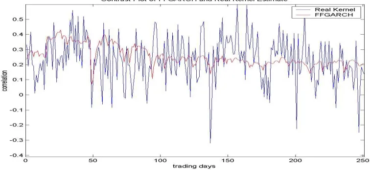
FGARCH(1,1,1) model and the real kernel estimate in the case that n=5. Time Period: All the trading days from Jan 1st, 2003 to Dec 31st, 2003. ... 67 Figure 2.2.4- 1 The contrast plot of the correlation between AIG and BAC by the FFGARCH model and the real kernel estimate in the case that n=2. Time Period: All the trading days from Jan 1st, 2003 to Dec 31st, 2003... 72 Figure 2.2.4- 2 The contrast plot of the correlation between AIG and BAC by the FFGARCH model and the real kernel estimate in the case that n=5. Time Period: All the trading days from Jan 1st, 2003 to Dec 31st, 2003... 72 Figure 2.2.4- 3 The contrast plot of the correlation between BAC and BAX by the

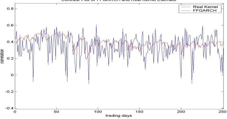
FFGARCH model and the real kernel estimate in the case that n=2. Time Period: All the trading days from Jan 1st, 2003 to Dec 31st, 2003. ... 73 Figure 2.2.4- 4 The contrast plot of the correlation between BAC and BAX by the

FFGARCH model and the real kernel estimate in the case that n=5. Time Period: All the trading days from Jan 1st, 2003 to Dec 31st, 2003. ... 73 Figure 2.2.4- 5 The contrast plot of the correlation between AIG and BAX by the FFGARCH model and the real kernel estimate in the case that n=2. Time Period: All the trading days from Jan 1st, 2003 to Dec 31st, 2003... 74 Figure 2.2.4- 6 The contrast plot of the correlation between AIG and BAX by the FFGARCH model and the real kernel estimate in the case that n=5. Time Period: All the trading days from Jan 1st, 2003 to Dec 31st, 2003... 74 Figure 2.2.4- 7 The contrast plot of the correlation between AMD and AAPL by the

x Figure 2.2.4- 8 The contrast plot of the correlation between AMD and AAPL by the

FFGARCH model and the real kernel estimate in the case that n=5. Time Period: All the trading days from Jan 1st, 2003 to Dec 31st, 2003. ... 76 Figure 2.2.5- 1 The contrast plot of the correlation between AIG and BAC by the

O-GARCH(1,1,n) model and the real kernel estimate in the case that n=2. Time Period: All the trading days from Jan 1st, 2003 to Dec 31st, 2003. ... 79 Figure 2.2.5- 2 The contrast plot of the correlation between AIG and BAC by the

O-GARCH(1,1,n) model and the real kernel estimate in the case that n=5. Time Period: All the trading days from Jan 1st, 2003 to Dec 31st, 2003. ... 79 Figure 2.2.5- 3 The contrast plot of the correlation between BAC and BAX by the

O-GARCH(1,1,n) model and the real kernel estimate in the case that n=2. Time Period: All the trading days from Jan 1st, 2003 to Dec 31st, 2003. ... 80 Figure 2.2.5- 4 The contrast plot of the correlation between BAC and BAX by the

O-GARCH(1,1,n) model and the real kernel estimate in the case that n=5. Time Period: All the trading days from Jan 1st, 2003 to Dec 31st, 2003. ... 80 Figure 2.2.5- 5 The contrast plot of the correlation between AMD and AAPL by the

O-GARCH(1,1,n) model and the real kernel estimate in the case that n=2. Time Period: All the trading days from Jan 1st, 2003 to Dec 31st, 2003. ... 81 Figure 2.2.5- 6 The contrast plot of the correlation between AMD and AAPL by the

O-GARCH(1,1,n) model and the real kernel estimate in the case that n=5. Time Period: All the trading days from Jan 1st, 2003 to Dec 31st, 2003. ... 82 Figure 2.2.5- 7 The contrast plot of the correlation between AIG and AMD by the

O-GARCH(1,1,n) model and the real kernel estimate in the case that n=2. Time Period: All the trading days from Jan 1st, 2003 to Dec 31st, 2003. ... 82 Figure 2.2.5- 8 The contrast plot of the correlation between AIG and AMD by the

O-GARCH(1,1,n) model and the real kernel estimate in the case that n=5. Time Period: All the trading days from Jan 1st, 2003 to Dec 31st, 2003. ... 83 Figure 2.2.6- 1 The contrast plot of the correlation between AIG and BAC by the

GO-GARCH model and the real kernel estimate in the case that n=2. Time Period: All the trading days from Jan 1st, 2003 to Dec 31st, 2003. ... 87 Figure 2.2.6- 2 The contrast plot of the correlation between AIG and BAC by the

GO-GARCH model and the real kernel estimate in the case that n=5. Time Period: All the trading days from Jan 1st, 2003 to Dec 31st, 2003. ... 87 Figure 2.2.6- 3 The contrast plot of the correlation between BAC and BAX by the

GO-GARCH model and the real kernel estimate in the case that n=2. Time Period: All the trading days from Jan 1st, 2003 to Dec 31st, 2003. ... 88 Figure 2.2.6- 4 The contrast plot of the correlation between BAC and BAX by the

1

Introduction

The distribution of financial variables has been the central interest of financial econometrics for a long time. In the early years, people did extensive research on the mean of a variable, the first moment of the distribution. For the second moment, variance and covariance, people were inclined to at first use the simple, convenient but implausible assumption that conditional variance and covariance were finite and constant over time. This assumption, however, was contradictory to the observed time varying volatility as Mandelbrot (1963) commented. Black and Scholes said (Black and Scholes, 1972) “... there is evidence of non-stationarity in the variance. More work must be done to predict variances using the information available.” See Shephard (2005) and Bollerslev and Engle (1993) for relevant comments. Then Engle’s famous GARCH model (1982) initiated the long prominence of time-varying volatility models, which shapes the current view of volatility in both the academic and empirical finance world.

2 Multivariate volatility analysis is also required for computing the optimal hedge ratio. The hedge ratio is the ratio of the size of the position taken in futures contracts to the size of assets exposed to market risk. For example, an airline wants to hedge the risk brought by price fluctuations (market risk) with futures contracts. Because there are no futures contracts on jet fuel available in the market, the company could only approximate them with heating oil futures (we call such a hedging strategy a crossing hedge). Then what fraction of risky assets should be covered? That is, what is the optimal hedge ratio? It will depend upon the correlation between the spot price change of jet fuel and the future price change of heating oil. A multivariate volatility model is useful in this case so that we can estimate the variance and covariance of price changes over time.

A similar application of the multivariate volatility model is used to estimate the beta coefficient in the Capital Asset Pricing Model (CAPM). Beta is the ratio of the covariance between individual asset return and market return to the variance of the market return. By using a multivariate volatility model, we can calculate both parts at the same time.

For portfolio management, multivariate volatility models are also popular. A portfolio consists of a bundle of assets. Regarding risk management, the portfolio manager has to evaluate the risk (measured by volatility) of the whole asset pool. A question that is always of interest is how the risk of a portfolio will change when we change the portfolio weights. To answer that we have to know all the covariances between the assets in the portfolio on top of all the variances. Multivariate volatility models can provide this information.

3 the continuous time framework, stochastic volatility models have gained much attention. Discrete time models also have flourished since the Autoregressive Conditional Heteroskedasticity (ARCH) model. In 1982 Robert Engle proposed the ARCH model, in which he assumed that the future volatility is a function of its present value and the squared returns. The ARCH model inspired many researchers’ approaches to volatility estimation and forecasting. A voluminous literature under this framework has emerged, such as the GARCH (Bollerslev 1986) model, the IGARCH model (Engle and Bollerslev, 1986), the EGARCH model (Nelson, 1991), etc. Given so many GARCH-type models, it is hard to compare their performance due to the lack of a good measure of the true volatility. Squared returns have long been used as a proxy but they turn out to be very noisy (Andersen and Bollerslev, 1998). Since the late 1990s thanks to the availability of high frequency data, a strikingly accurate measure of the true volatility has been modeled with a new methodology: the Realized Volatility model. The major contributors to this methodology include Andersen, Bollerslev, Diebold, and Labys (2001) and Barndorff-Nielsen and Shephard (2002). They originally utilized the ultimately detailed information (for example, TAQ data includes the record of every single trade or quote in one day on the NYSE) to measure the true volatility over a period of time based on a continuous-time stochastic volatility framework.

4 Correlation (DCC) model by Christodoulaskis and Satch (2002), Engle (2002) and Tse and Tsui (2002), and the General Dynamic Covariance (GDC) model by Kroner and Ng (1998). On the other hand, the realized volatility models also manage to provide corresponding measurement of the true covariances and correlations, despite challenges such as micro-structure noise and non-synchronous trading of high frequency data. Andersen, Bollerslev, Diebold and Labys (2003) developed a bi-variate realized co-volatility model as a natural generalization of the univariate realized volatility when they analyzed the exchange rates of DKK/$ (the abbreviation of Denmark currency Danish Kroner) and Yen/$. Barndorff-Nielsen, Hansen, Lunde and Shephard (2006) proposed the Real Kernel model which addressed the micro-structure noise problem. In their later papers (2008) and (2011), they not only expanded the model to multiple dimensions, but also improved it to be immunized against non-synchronous trading and ensured that the obtained covariance matrices are semi-definite positive.

5 processes during the estimation of realized measures. Shephard and Sheppard (2010) proposed the HEAVY model which is nested in the MEM class of models. Hansen, Lunde and Voev (2010) developed the realized Beta GARCH model. Hansen, Huang and Shek (2011) introduced a univariate GARCH-X model with a measurement equation to address multiple-period forecasting. Realizing the fact that the existing models have only solved some of the encountered problems, we develop a model to address more challenges in a single model. The new member we introduce to the multivariate volatility family is called the Real Dynamic Conditional Correlation, which adds a measurement equation. It is based on a traditional MGARCH model, the Dynamic Conditional Correlation (DCC) model of Engle (2002), after carefully comparing the ten most popular traditional MGARCH models. The performance is superior to its pioneers due to the inclusion of a realized volatility term and a measurement equation. For the proper formulation, the model controls the number of parameters to estimate so that the dimension curse is not a concern. Modeling details will be shared in the last chapter.

6 model. In section 1.6 we give a brief conclusion about the current multivariate volatility study.

7

Chapter 1 Review of GARCH Modeling and Realized Volatility Literature

1.1 Introduction

As a generalization of Engle’s famous ARCH model (1982), the GARCH model proposed by Bollerslev (1986) formulates the latent volatility as an autoregressive function of its past values and past squared returns. A simple GARCH(1,1) model can be described as,

1/ 2

t t t

y  h , ℎ𝑡 = 𝜔 + 𝛼𝑦𝑡−12 + 𝛽ℎ𝑡−12 , 𝜀𝑡~𝑁𝐼𝐼𝐷(0,1) (1.1.1) A straight-forward conclusion is 𝐸𝑡−1(𝑦𝑡2) = ℎ𝑡 due to the conditional mean of yt being

zero. To test this condition, a Mincer-Zarnowtiz style regression can be conducted: y_t2 ₀₁h_t _t , E( ) 0 _(1.1.2) Test 𝛽 = 0, 𝛽₁ = 1 v.s. 𝛽₀ 0 or 𝛽₁ 1.

Such a type of regression is to regress the actual variable on its fitted counterpart to test whether a model provides consistent estimate to the actual variable. In our case, we use the squared daily return as the proxy of actual volatility and take the estimated volatility from the GARCH model as independent variable. We do not reject for such type of regressions in many researches. See Bollerslev et al. (1992), Bollerslev et al. (1994), Ghysels et al. (1996) and Shephard (1996). But they also found that the variation of estimated volatility ℎ𝑡 explained little of the variation of the ex-post squared returns 𝑦_𝑡2_{. That is, the 𝑅}2 _{of such} regressions is low. Bollerslev interpreted such low 2

R as the result of a magnified effect of the error term 2

t

 contained in squared returns, keeping in mind that 2 2

t t t

8 less noisy estimate of the actual volatility, they put aside the squared returns as a proxy, and proposed a new measure, realized volatility.

1.2 The Realized Volatility

The Realized Volatility (RV) was first coined by Andersen and Bollerslev (1998). They tried to use it to get a less noisy measurement of the true volatility than the squared daily return. As we saw in the first section, large variation in the squared return may be the result of large variation in the error terms instead of the true volatility, even if the volatility forecasted by GARCH is pretty precise, it can still render a seemingly low 𝑅2 in the Mincer-Zarnowitz regression.

Barndorff-Nielsen and Shepard (2002) presented theoretical inference for the Realized Volatility method. We will follow their notation.

The asset price (take log) we can observe in the real world is in discrete time, denoted by 𝑦 . Given a fixed time interval of length ℎ 0, we denote the return over the ℎ interval as,

𝑦 = 𝑦 ( ℎ) 𝑦 (( 1)ℎ), = 1, , (1.2.1)

For example, if ℎ represents a day, 𝑦 is the daily return; if ℎ represents a week, 𝑦 is the weekly return. Then by evenly dividing the time interval of ℎ into M pieces, the ℎ intra-h return at the ℎ time interval is,

𝑦 , = 𝑦 (( 1)ℎ + ) 𝑦 (( 1)ℎ + ( −1)) , = 1, , , (1.2.2)

We can define the realized variance for day as,

𝑦 = ∑ ₁𝑦 _, 2 (1.2.3)

9

√∑ 𝑦 _, 2

1 (1.2.4)

If we could prove that the realized volatility as defined above is a consistent estimate of the true volatility, we would substitute it for the squared return as the proxy of the true volatility. Next we will take a look at Barndorff-Nielsen and Shephard’s inference results for the asymptotic properties of the realized volatility.

Their proof starts from the assumption that the true price generating process is a semi-martingale,

𝑦 ( ) = 𝛼( ) + ( ) t0 _(1.2.5)

where 𝑦 ( ) is log-price at time t, 𝛼( ) is a drift term, ( ) is a local martingale.

This specification implies two assumptions. First, we consider the continuous-time model as an approximation of the empirical discrete world. Given the voluminous trading of financial assets in the exchange nowadays, we believe this is a proper approximation. Second, 𝑦 ( ) is a special semi-martingale, where 𝛼( ) is the predictable finite variation process so that the decomposition in (1.2.5) is unique. We would like to briefly interpret the concepts of martingale, local martingale and semi-martingale. (See Protter, 1990).

Martingale: A real valued, adapted process = ( _𝑡) _𝑡 is called a martingale with respect to the filtration ( _𝑡) _𝑡 if

𝐸{| 𝑡|} and if , then 𝐸{ 𝑡| } = .

non-10 zero expectation of the future shocks in price has been arbitraged immediately, the martingale assumption about the asset price is reasonable.

Local martingale: An adapted, càdlàg process X is a local martingale if there exists a sequence of increasing stopping time, , with = a.s. (almost sure) { _𝑡 } is a martingale, where = ( , ). We can see from the definition that martingale is a special case of local martingale where = All martingales are local martingales but not vice versa.

Semi-martingale: A process is a semi-martingale if it can be decomposed as a process with finite variation and a local martingale. A process is a finite variation process if all its realizations have finite variation. We call the semi-martingale special here because the process with finite variation 𝛼( ) is predictable (e.g. the process has a deterministic trend).

According to the CAPM theory, an asset price can be decomposed into a riskless part and a risky part. Then it is natural to see the riskless part as the predictable process 𝛼( ) with finite variation path and the risky part as ( ), the local martingale process. By limiting ourselves to the special semi-martingale we can ascertain that such a decomposition is unique, otherwise we cannot identify where the stochastic change of prices comes from.

Barndorff-Nielsen and Shepard (2002) made a further assumption about the specification of ( ) but we would like to hold the introduction of this assumption until it is necessary. The realized volatility is defined as,

1

* * * 2

1 0

[ ] { ( ) ( )}

M

M j j

j

y y s y s



 





Where0   s₀ s₁ ... s_M t, ₁

11 The squared return from j to j+1 is equal to,

{𝑦 ( 1) 𝑦 ( )}2

= 𝑦 2₍

1) 𝑦 ( 1)𝑦 ( ) + 𝑦 2( )

= 𝑦 2₍

1) 𝑦 2( ) + 𝑦 2( ) 𝑦 ( 1)𝑦 ( )

= 𝑦 1 2 𝑦( )(𝑦( 1) 𝑦( )) (1.2.7)

so that we know the realized volatility has the asymptotic property, ∑ −1 {𝑦 ( 1) 𝑦 ( )}2 = ∑ −1 𝑦 1 2 𝑦 ( ) 𝑦 1 and

∑ −1 𝑦 1 2 𝑦 ( ) 𝑦 1 𝑦 2+ 𝑦𝑡 2 ∫ 𝑦𝑡 ( ) 𝑦 ( ) as . (1.2.8)

The equation 𝑦 2+ 𝑦_𝑡 2 ∫ 𝑦𝑡 ( ) 𝑦 ( ) is exactly the definition of the quadratic variation of a semi-martingale. Here we assume that 𝑦 = 0. More details about the quadratic variation can be found in Protter (1990, pp. 58~59). All the derivations just prove that the realized volatility is a consistent estimator of the quadratic variation. But even if we know the fact above, what is the relevance of the realized volatility to the actual variance of 𝑦_𝑡? Next we will prove if we take *

t

y as the combination of a continuous component and jumps, and rewrite the quadratic variation as,

𝑦 ( ) = 𝑦 _{( ) + ∑ {𝑦 ( ) 𝑦 ( )}}2

𝑡 (1.2.9)

where y*cdenotes the continuous component of * t

12

𝑦 ( ) = 𝑦 _{( ) + ∑ { 𝛼( )}}2

𝑡 + ∑ 𝑡{ ( )}2+ ∑ 𝑡 𝛼( ) ( )

= 𝛼 ( ) + ( ) + ∑ { 𝛼( )}2

𝑡 + ∑ 𝑡{ ( )}2 ∑ 𝑡 𝛼( ) ( ). (1.2.10) Here 𝛼 ( ) = 0 because a continuous local martingale with finite variation is constant. The quadratic variation of a constant is zero (Protter, 1990, pp. 64). Given the assumption that ( )t is predictable without any jumps, the items containing 𝛼( ) on the right hand side are both equal to zero. Then the equation (1.2.10) can be simplified as,

𝑦 ( ) = ( ) (1.2.11)

where ( ) = ( ) + ∑ 𝑡{ ( ) ( )}2 similar to the expression in (1.2.9). That is to say, the variation of a semi-martingale comes from the variation of the local martingale part. At this stage, however, we haven’t obtained any information about whether the realized volatility is a consistent estimator of the true variance. Could the quadratic variation of the local martingale be the variance of the semi-martingale? The answer is “yes” if we add the final assumption that the price 𝑦 ( ) follows a stochastic volatility process, which is a sub-segment of the semi-martingale class. This assumption allows for time-varying volatility. Based on those three assumptions, we can take a look at what the realized volatility estimates. Given the assumption above we have,

0

( ) t ( ) ( ) m t 



(1.2.12)

( ) = ∫ ( ) ( )𝑡 ( )

= {∫ ( ) ( )𝑡 }2_{+ ∬ (}

1) ( 2) ( 1) ( 2)

𝑡

. (1.2.13)

13

∬ ( 𝑡 1) ( 2) ( 1) ( 2)= 0 .

We can see from the equation (1.2.13) that,

( ) = ∫ 𝑡 2_{( ) (1.2.14)}

The item on the right-hand side of the equation above is exactly the variance of * t

y , denoted by*2( )t . Combined with results obtained previously, the realized volatility is

* * *2

[y_M]( )t [y ]( )t [ ]( )m t  ( )t as M   _(1.2.15) It is theoretically proved that realized volatility is a consistent estimator of the integrated variance of asset returns. Andersen and Bollerslev (1998) hence claimed that volatility can be treated as an observable variable from then on. If we increase M to a very large number, the realized volatility estimation will be so precise that we can proceed as if we observe the actual variance directly.

14 proxy of the true volatility. Treating the realized volatility as the observed volatility, Andersen et al. (2001) also applied it to the VAR(5) model to forecast the future volatility and compared the forecasts with those obtained from GARCH(1,1) and other GARCH type models to find that the VAR-RV model had more explanation power. For a thorough report about the volatility study of DKK/$ and Yen/$ data, one can refer to Andersen et al. (2001).

The idea behind the realized volatility is simple. It uses quadratic variation to measure the variance of asset returns, hence converts the estimation of volatility to a problem of integration. Access to the high frequency data makes this strategy feasible. Andersen and Bollerslev along with others who pioneered this field believe the volatility can be treated as an observable variable from then on, whenever it is needed in financial applications.

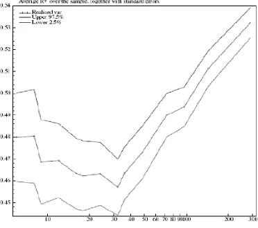
15 Figure 1. 1 Average (across days) value of the RV drawn against M.

Taking M over 50, we can find the previously decreasing RV rises significantly. This result is considered as an indicator of the presence of the market microstructure noises. To avoid them, Andersen and Bollerslev (1998) chose to sample at an intermediate frequency like every 5 minutes or even 30 minutes although data can be observed almost every few seconds. A new problem arises if we do so. If the sample isn’t selected frequently enough, the estimates gained from RV won’t be close to the true value. A closer look at the distribution of RV can provide some theoretical perception on the accuracy loss.

16

𝑦 ( )= 𝛼( )+∫₀ ( ) ( ) (1.2.16)

which is driven by a Wiener process. So we can see that

𝑦 ( )|𝛼( ), 2_{( )~𝑁(𝛼( ),} 2_{( )) (1.2.17)}

where *2 2

0

( )t t ( )s ds

 



in Barndorff-Nielsen and Shephard (2002), the asymptotic distribution of RV is,

2 2 , ( 1) 1 4 ( 1) ( ) (0,1)

2 ( )

M _hi j i h i j hi h i

M y s ds

N

h s ds

          







, _{( 1)}

1 4 , 1 ( ) (0,1) 2 3 M _hi

j i _{h i} j

M j i j

y s ds

N y      







as M   _(1.2.19)

and

4 4

, _{( 1)} 1

( ) 3

M _hi

j i _{h i} j

M

y p s ds

17 Another problem encountered with the RV method is the irregular transaction durations. Realized Volatility is usually calculated on a fixed time interval to study the asymptotic property, therefore people need to implement interpolation at fixed time points where there is no trade occurring. Such a strategy could be problematic if the asset is not traded actively in which case the continuous-time assumption is not appropriate because of the presence of sizable discreteness. It is commonly accepted that the duration between trades is correlated with the volatility. Longer duration between adjacent transactions tends to accompany a larger volatility of the price. Simply interpolating the price will miss that useful information. We should find a way of dealing with such endogenous sampling interval. Barndorff-Nielsen, Hansen, Lunde, and Shepard (2006) discussed the asymptotic distribution of RV calculated on irregularly spaced time intervals.

1.3 The Real Kernel Model

18 The real kernel estimator has the following form,

̃( ) = ( ) + ∑ ₁ ( −1){ ( ) + − ( )} (1.3.1)

where is a log price process, is a fixed time interval, and ( ) denotes the ℎ ℎ realized autocovariance,

( ) = ∑ 1( ( −1))( ( −1) ( − −1) ), = ⁄ (1.3.2)

The scalar denotes a very small time period so that we can think of ( _{( −1)}) as the ℎ high frequency return and represents a single interval. The first item on the right-hand side of (1.3.1) is the realized volatility we have discussed in detail in the previous section. The second item is the correction for micro-structure noises. We will pay much attention to the kernel function ( ) ( 0,1 ), where the name real kernel comes from. The kernel function is so important that its characteristics decide the essential properties of the estimator such as asymptotic efficiency and convergence rate.

Keep in mind that the observed log-price process X is contaminated by market micro-structure noise. That is,

= + (1.3.3)

Where is true log price that we cannot observe and denotes the market micro-structure noise. The variable is assumed to be a white noise process independent of . 𝐸( _𝑡) = 0,

( _𝑡) = 𝜔2_{, (}

19 case noise from bid-ask spread reduced. Some other stocks may have noise from trading information lag. The effect of those noises is different across the stocks and changes over time. When we do multivariate analysis for multiple assets, we need to decompose the observable stock prices of those assets into the true price part and the noise part to make sure the comparison is independent of the noises included in those prices. The real kernel estimator ̃( ) is proven to be consistent given the presence of if the kernel function is flat top. A flat top kernel means that the kernel function is ( −1) not ( ). The difference in the two specifications makes essential changes to the properties of the real kernel estimator in the presence of market micro-structure noise. If we define the kernel function as ( ), then it can be shown that 𝐸{ ̃( )} = 𝜔2 {1 (1)} 0. And the estimator will be biased. So we impose the flat top constraint on the kernel function ( ). The proof is briefly summarized here.

To begin with the proof, we first present some definitions that will be used later. We adopt the notation from Barndorff-Nielsen, Hansen, Lunde and Shephard (2006). For any process X and Z, we define

( , ) = ∑ 1( ( −1) )( ( − ) ( − −1) ), ℎ = , , 1,0,1, , , (1.3.4)

and ( ) = ( , ) . Given (1.3.3) we will see that,

( ) = ( ) + ( ) + ̃( , ) (1.3.5)

where ̃( , ) = ( , ) + ₋ ( , ). Substituting (1.3.3) and (1.3.5) into the real

kernel estimator formulation (1.3.1), we get Substituting (1.3.3) and (1.3.5) into the real kernel estimator formulation (1.3.1), we get

20 For future convenience, we define the realized auto-covariance vectors as the follow,

( ) = { ( ), 1( ), , ( )} , ̃( ) = { ( ), ̃ ( 1 ), , ̃( )} ,

̃( , ) = { ( , ), ̃ ( 1 , ), , ̃( , }

and a weight (kernel) vector defined below also helps to write the real kernel estimator ̃( ) in a convenient form so its asymptotic properties are easier to illustrate:

𝜔 = (1, 1, (1) , , ( −1)) .

Given all the auto-covariance vectors and weight vector, we can rewrite (1.3.1) as,

̃( ) = 𝜔 ̃( ) (1.3.7)

and (1.3.6) can be rewritten as,

̃( ) = 𝜔 ̃( ) + 𝜔 ̃( ) + 𝜔 ̃( , ) (1.3.8)

The equation (1.3.8) is an important formula because the asymptotic properties of the real kernel estimator ̃( ) are deduced from the items on its right hand side. Given the assumptions about the market micro-structure noise 𝑡, we expect the second and third item on the right asymptotically to have a mean equal to zero. Barndorff-Nielsen, Hansen, Lunde and Shephard (2006) provide a theorem that helps to depict the distributions of those items. Theorem 1 Suppose that is a Brownian semi-martingale and the stochastic volatility is a function with constant volatility plus some adapted càdlàg processes, then as 0 ,

−

(

∫ 𝑡 2

1( )

( ) ₎

𝑁 (0, ∫ 𝑡 ) , = (

0 0 1

0 0

0 0 1

21 where is the realized volatility calculated on fixed time interval, MN denotes mixed normal distribution and LS represents convergence in law stably.

For the third item on the right hand side of equation (1.3.8), if 𝑁 and then

̃( , ) 𝑁(0, 𝜔 2 _{) (1.3.10)}

Where is a ( + 1) ( + 1) symmetric matrix with block structure, = ( 11 12 21 22),

22 = ( 1

0 1

) , ₁₁= ( 1

1 ) , 21= (

0

0 10

0 0

) , ₁₂= ₂₁and ₂₂ is a

( 1) ( 1) symmetric matrix.

When is white noise and = ⁄ , for

𝐸{ ( )} = 𝐸{ ̃( )} = 𝜔2 _{(1, 1,0,0, ,0) , { ̃( )} = 𝜔 ( + 𝐷̃)}

where ( + 1) ( + 1) symmetric matrices and 𝐷̃ have a block structure,

= ( 11 12

21 22) , 𝐷̃ = (𝐷

̃_{11 𝐷}̃₁₂

𝐷̃₂₁ 𝐷̃₂₂)

where the ( 1) ( 1) and ( 1) dimensional matrices are,

22= ( 1 0 1 )

, 21 =

( 1 0 0 1 0

0 _{0 )}

𝐷̃₂₂ =

( 10 0 0 0 1

10 1

2 1)

, 𝐷̃₂₁=

( 1 0 0 0

0 _{0 )}

22 with 12= 21, 𝐷̃12= 𝐷̃21, ℎ 11, 𝐷̃11

11 = ( 1 +

2 2

2 ₊ 2 ) , 𝐷̃ = (11

2 _{1 +} 2

1 + 2

2

)

For conciseness, the details of the derivation of those matrices based on asymptotic theory won’t be covered here. With all the information about the items on the right at hand, we now know that ̃( ) ∫ 𝑡 2 should asymptotically have a mixed normal distribution with zero mean and its variance should be determined by A, B,C, and 𝐷̃.

Theorem 2 Given the kernel (weight) vector 𝜔 = (1, 1, (1) , , ( −1)

we assume that the kernel weight function ( ) is four times continuously differentiable. As H increases, the flat-top kernels have

𝜔 𝜔 = , _{+ (1),}

𝜔 𝜔 = −1_{{ (0) +} ,2_{} + (} −2_),

𝜔 𝜔 = −2_{{ (0)}2_{+ (1)}2_{} +} − _{{ (0) +} , _{+ (} − _),

𝜔 𝐷̃𝜔 = −1_{{ (0) +}1

2

( ) ₊ ,2_{} + (} −2_),

where , = ∫ ( )1 2 , ,2= ∫ ( ) ( )1 , , = ∫ ( ) ( )1

Looking back to (1.3.8), we will see that asymptotic variance of ̃( ) ∫ 𝑡 2 can be written as,

( ̃( ) ∫ 𝑡 2 _{) = 𝜔 ( ̃( ))𝜔 + 𝜔 ( ̃( ))𝜔 + 𝜔 ( ̃( , ))𝜔}

23 From equation (1.3.9) we know that

−

(

∫ 𝑡 2

̃1( )

̃ ( ) ₎

𝑁 (0, ( 0

0 0 0

0 0

) ∫ 𝑡 ) (1.3.12)

We then know that,

𝜔 ( ̃( ))𝜔 = ∫ 𝑡 2 𝜔 𝜔 = −1_∫ 𝑡 2 , _(1.3.13)

𝜔 ( ̃( ))𝜔 = 𝜔 ( 𝜔 𝜔 + 𝜔 𝐷̃𝜔) = 𝜔 −2_{{ (0)}2_{+ (1)}2_{} +}

− _{{ (0) +} , _{} 𝜔} −1_{{ (0) +}1

2 (0)

2₊ ,2_{} (1.3.14)}

𝜔 ( ̃( , ))𝜔 = 𝜔2_∫ 𝑡 2 _{𝜔 𝜔 = 𝜔}2_∫ 𝑡 2 −1_{{ (0) +} ,2_}

(1.3.15) Summing (1.3.13), (1.3.14) and (1.3.15) together and combining the same items,

( ̃( ) ∫ 𝑡 2 ₎₌ −1_∫ 𝑡 , −1_{{ (0) +} ,2_{} { 𝜔}2_∫ 𝑡 2 ₊

𝜔 } + 𝜔 −2_{{ (0)}2_{+ (1)}2_{} +} − _{{ (0) +} , _{} 𝜔} −1 1

2 (0)2 (1.3.16)

Theorem 2 shows that the variance of ̃( ) ∫ 𝑡 2 is a function of H. If we relate H to

= ⁄ , , it is equivalent to associating the convergence rate to the choice of H.

24

1 _{{ ̃( ) ∫} 𝑡 2 _{} 𝑁 0,} , _∫ 𝑡 −1 ,2_𝜔2_(∫ 𝑡 2 ₊

2) +

𝜔 − _{{ (0) +} , _{} (1.3.17)}

We can see that the convergence rate is 1 , which is the best convergence rate achieved. As we mentioned above, c is chosen to minimize asymptotic variance of the real kernel estimator. So c should be a function of the kernel function ( ). then is determined as,

= , = √ 1 , { ,2+ √( ,2)

2

+ , } ℎ = (0) + , (1.3.18)

and the corresponding optimal variance is,

( , −1 ,2₊ − _{) 𝜔 = 𝜔 (1.3.19)}

Different types of kernel functions will return different derivatives and integrals. By assuming (0) = 0 (1) = 0, the convergence rate will be the fastest. The authors have selected the Modified Turkey-Hanning kernel which achieves the highest asymptotic efficiency. That is the kernel used in our data analysis.

To obtain a feasible value of , we need to find the estimates of 𝜔 , which are also provided in Barndorff-Nielsen, Hansen, Lunde and Shephard (2006). The variance of market micro-structure noise 𝜔 is given as, 𝜔̂ = 2 , where is realized volatility computed with a very small time interval , such as 1 minute, and ̂ = 2 ₁ where ₁ is low-frequency realized volatility, say, a 10-minute interval. Usually we don’t think market micro-structure noise is included in low-frequency realized volatility.

25 time interval . In Barndorff-Nielsen, Hansen, Lunde and Shephard paper (2006), they proved that a real kernel estimator calculated with tick time data (stochastically spaced) is also consistent for the true volatility.

We have assumed that the log-price process is a Brownian semi-martingale with its spot volatility expressed by _𝑡2 = ∫ 𝑡 2 . Now we add another stochastic process T, consisting of the observable trading times. T has the form of _𝑡 = ∫ 𝑡 2 , with having strictly positive, càdlàg sample paths and = , = 1, , , By defining a new process written

as = , we mean = , = 1, , , for j-th measurement time. The interval

denotion in this context means the fixed number of trades that actually happens. For example, if on average there are 5 trades occurring within 1 minute then the real kernel estimate calculated with irregular spaced returns of every 5 trades corresponds to that calculated with evenly spaced returns of every 1 minute. The following proposition will show that with spot volatility 𝑡, which is consistent with the results obtained by Mykland and Zhang (2006).

Proposition Let _𝑡 = _𝑡 and _𝑡 = ∫ 𝑡 2 then is a càdlàg process and = , where is the stochastic volatility of the Z process. This implies that for the real kernel, we can write an irregularly spaced version of the log-price process _𝑡 such as

𝑡 = ∫ 𝑡 + ∫ 𝑡 (1.3.20)

26 ( )_𝑡= ( )_𝑡+ ∑ ₁ ( −1){ ( )_𝑡+ ₋ ( )_𝑡} (1.3.21)

with ( )_𝑡= ∑[ ₁] ( _{( −1)})( _{( − ) ( − −1)}) .

This version of the real kernel estimator is the one we use in our data analysis. To calculate roughly 1-minute real kernel estimates, we first calculate the average number of trades occurring during one minute and then select prices every x trades (number of trades occurring within 1 minute on average) and then computed the real kernel estimator based on these irregularly spaced prices.

Barndorff-Nielsen, Hansen, Lunde and Shephard (2006) did both simulation studies and empirical analysis to study the properties of the real kernel estimator. They utilized high frequency data on General Electric (GE) stock prices in 2004 for the empirical analysis. The results, just as expected, show that the real kernel estimator has remarkably smaller confidence intervals than the realized volatility at high frequency (roughly 60 seconds). Proven to be a good starting point, the real kernel estimator was generalized to the multivariate case by Barndorff-Nielsen, Hansen, Lunde and Shephard (2011). In that paper, the non-synchronous trading problem is addressed and a multivariate real kernel estimator is introduced. Now we briefly introduce this multivariate real kernel estimator.

1.4 The Multivariate Real Kernel Estimator

27 NYSE, so the observation times we refer to here are all actual trading times. For the i-th asset the trading times are ₁( ), ₂( ), , which means that for i-th asset its price should be written as ( )₍ ( )_{) for = 1, , , 𝑁}( )_{. As they proved for the univariate case, the real kernel} estimator is consistent even with a trade-based price process. But how should we synchronize trading time as a starting point of multivariate real kernel estimator computation? Barndoff-Nielsen, Hansen, Lunde and Shephard (2011) proposed the concept of “Refresh Time” to solve this problem.

Definition 1 Refresh Time for 0, 1 Define the first refresh time as ₁ = ( ₁(1), , ₁( )), and then subsequent refresh times as

1= (

( ) 1

(1) _{, ,}

( ) 1

( ) ₎

(1.4.1)

28 Figure 1.4- 1 Multivariate real kernel data series alignment

After synchronizing the return vector { }, we define the multivariate real kernel estimator as,

( ) = ∑ ₋ ( ) , (1.4.2)

where = ∑ _{1 −} ℎ 0, = ₋ ℎ 0. The properties of the kernel function ( ) are essential to determine the asymptotic distribution and positive-definiteness of the estimator. Here are some assumptions about the kernel function ( ):

( ) (0) = 1, (0) = 0 (1.4.3)

( ) ℎ (1.4.4)

( ) , _{= ∫ ( )}2 _, 1,1 _{= ∫ ( ) ,} 2,2 _{= ∫ ( )}2 _(1.4.5)

, _, 1,1_, 2,2

29 It is easy to see that the assumption (0) = 1 in ( ) is to give unit weight to . (0) = 0 means the real kernel estimator gives long-lag auto-covariances a smaller weight. ( ) is set to guarantee that the real kernel estimator is positive definite.

The inference with the multivariate real kernel estimator shares a lot of characteristics with its univariate counterpart. We won’t repeat the shared part here but will focus instead on the differences. In the univariate case Barndorff-Nielsen, Hansen, Lunde and Shephard (2006) recommends the Modified Tukey Hanning kernel function while for the multivariate case, they found a Parzen type kernel can guarantee the estimator to be positive definite.

Another difference lies in the assumption of market micro-structure noise. In the univariate case, they assumed the noise to have an i.i.d distribution of noises, that is, So they were reluctant to select data at a frequency higher than once every minute. In the multivariate case, they adopt a larger bandwidth H so that tick-by-tick data can also be considered. The new bandwidth in the multivariate case is specified as = ( ₁, , ) with = for = 1, , , where = {

( )

, }1 , 2 =_√

. The numerator

is the estimate of the variance of market micro-structure noise for asset i and √𝐼 is the corresponding estimate of square root of the integrated quarticity ∫ 𝑡 , which is approximated by the low-frequency realized volatility in the empirical analysis. is a constant equal to 3.51 for the Parzen kernel.

30 Given the availability of such an accurate estimate of the true volatility as the real kernel estimator, now we can do research on some topics that are interesting but were not feasible before. For example, is there any MGARCH model that outperforms its peers? Until recently we didn’t have a reliable measurement of the true volatility with which we could compare the MGARCH model estimates. But now we have seen that the real kernel estimator is a good measure of the true volatility and all the MGARCH model estimates can be compared with the real kernel estimator. Another question is whether we can develop a MGARCH based model that integrates the real kernel estimator of the true volatility if we do find an outperforming traditional MGARCH model. That is, we want to use the real kernel estimator as a term in the modeling function. We will briefly review ten of the most popular MGARCH models in this chapter and in Chapter 2 we will provide an empirical analysis comparing their performance at forecasting future volatility, taking the real volatility as a criterion.

1.5 The Multivariate GARCH (MGARCH) models

We specify a GARCH(1,1) model as,

𝑦𝑡= 𝜀𝑡ℎ1 2 (1.5.1)

where 𝐸_𝑡−1 𝜀_𝑡 = 0 and _𝑡−1 𝜀_𝑡 = 𝐼 with = 1.

When we deal with the multivariate case, that is, 1, we rewrite (1.5.1) as the following,

𝑦𝑡= 𝑡1 2𝜀𝑡 (1.5.2)

where the conditional covariance matrix _𝑡 is a positive definite matrix, whose square root can be calculated with the Cholesky decomposition, and

31 through their specification of _𝑡. They can be classified into three categories. The first category is a direct generalization of the univariate GARCH model including the VEC, the BEKK and the factor model; The second category contains Orthogonal models and Latent Factor models; The last category includes the Constant Conditional Correlation (CCC) model, the Dynamic Conditional Correlation (DCC) model and the General Dynamic Covariance (GDC) models. See Bauwens, Laurent and Rombouts (2006) for a survey of some of these models. For simple notation, all the models are reviewed in (1,1) forms.

Model 1 The VEC(1,1) model by Bollerslev et al. (1988) can be defined as,

ℎ𝑡 = + 𝑡−1+ ℎ𝑡−1 (1.5.3)

Where ℎ𝑡 = ℎ( 𝑡) 𝑡 = ℎ(𝑦𝑡𝑦𝑡 ) and ℎ( ) represents the operator stacking the lower triangular portion of a matrix as a ( + 1) 1 vector. The matrices A and G are square parameter matrices of order ( + 1) and is a ( +

1) 1 parameter vector. So the total number of unkown parameters is ( +

1)( ( + 1) + 1) . That is to say, even a bi-variate VEC(1,1) model can have 21

parameters, a tri-variate VEC(1,1) model will have 78 parameters to estimate, which is not feasible for high dimension. The simplified VEC model, Diagonal VEC (DVEC) model by Bollerslev et al. (1988), assumes A and G are diagonal matrices, which reduced the number of parameters to ( + ) . Besides, to guarantee a positive definite _𝑡, DVEC is expressed in terms of Hadamard products (denoted by ),

32

, and are symmetric matrices, where = ℎ( ) ,

= ℎ( ) and = ℎ( ). _𝑡 is positive definite if A, G and C along with the

initial variance matrix are positive definite.

The BEKK model (1995), a synthesized work of Baba, Engle, Kraft and Kroner, guarantees a positive definite covariance matrix _𝑡 without the restriction of positive parameter matrices.

Model 2 The BEKK(1,1,k) model is specified as,

𝑡 = + ∑ 1 𝑦𝑡−1𝑦𝑡−1 + ∑ 1 𝑡−1 (1.5.5)

where , and are matrices and is upper triangular.

The total number of parameters to estimate for the BEKK(1,1,k) model is ( ( + 1) +

1) .

We can see both the VEC and the BEKK models have to deal with a large number of unknown parameters. The next model to be reviewed, the Factor model by Engle et al. (1990), overcomes this problem by assuming that “co-movement of stock returns are driven by a small number of common underlying variables” (Bauwens, Laurent and Rombouts 2006).

Model 3 The Factor-GARCH(1,1,k) model .

The BEKK(1,1,k) model is called the Factor-GARCH(1,1,k) model if for k=1,2,…,K,

have rank one and have the same left and right eigenvectors, 𝜔 , i.e.,

= 𝛼 𝜔 and = 𝛽 𝜔 (1.5.6)

33 𝜔 = {0 _{1 =} ∑ 1𝜔 = 1

Substitute (1.5.6) into (1.5.5) to obtain,

𝑡 = + ∑ 1 (𝛼2𝜔 𝑦𝑡−1𝑦𝑡−1 𝜔 + 𝛽2𝜔 𝑡−1𝜔 ) (1.5.7)

We can see from (1.5.7) that the number of parameters in the F-GARCH(1,1,K) model is

( + + 1) , much less than ( ( + 1) + 1) in the BEKK(1,1,k) model. A variant

of the factor model is the Full-Factor GARCH model proposed by Vrontos et al. (2003). Model 4 The FF-GARCH model is defined as,

𝑡 = 𝑡 (1.5.8)

where is a lower triangular parameter matrix with ones on the diagonal, _𝑡= ( _1,𝑡2 _{, ,}

,𝑡2 ) where ,𝑡2 is the conditional variance of the factors. The factors, −1𝑦𝑡 , follow separate univariate GARCH processes. The total number of parameters to estimate is

( + ) . There are some other models than those we have discussed above. They are not

directly generalized from the univariate GARCH model. Now we will take a look at the models from the second category of the MGARCH model family.

First we will introduce the Orthogonal GARCH model, which assumes the 1data vector is the orthogonal transformation of (or fewer) univariate GARCH processes.

Model 5 The O-GARCH (1, 1, m) model by Kariya (1988) and Alexander and Chibumba(1997) is defined as,

−1 2_𝑦

34 where = ( ₁, ₂, , ), with the population variance of 𝑦 _𝑡, and is a

matrix, , = ( ₁ ) , ₁ , which are the largest m eigenvalues of

the population correlation matrix _𝑡, and is the matrix of associated eigenvectors.

𝑡 = ( 1𝑡, , 𝑡) is the vector whose volatility follows a GARCH (1,1) process such that,

𝐸𝑡−1( 𝑡) = 0 𝑡−1( 𝑡) = 𝑡= ( 1𝑡2 , , 𝑡2 )

𝑡2 = (1 𝛼 𝛽) + 𝛼 ,𝑡−12 + 𝛽 ,𝑡−1 ,𝑡−12 = 1, , , (1.5.10)

𝑡 = 𝑡−1(𝑦𝑡) = 1 2 𝑡 1 2 ℎ 𝑡= 𝑡−1( 𝑡) = 𝑡 (1.5.11)

The number of parameters in the O-GARCH model, in the case of m=n, is equal to . The advantage of the O-GARCH model lies in the fact that it uses a small number of principal components (Alexander and Chibumba take m=2 for 12 assets), which reduces the computation burden. This scheme, however, also has drawbacks. For instance, if m<n, the rank of 𝑡 is m, not full rank. The diagnostic test will, however, rely on the inverse of 𝑡. So Weide (2002) proposed the Generalized Orthogonal(GO) GARCH model, where orthogonal assumption is replaced by assuming is square and invertible.

Model 6 The GO-GARCH(1,1) model is defined as Model 5, where m=n and is a non-singular matrix of parameters. The conditional correlation matrix of 𝑦_𝑡 is,

𝑅_𝑡 = _𝑡−1

𝑡 𝑡−1, ℎ 𝑡 = ( 𝑡 𝐼 ) 1 2 𝑡= 𝑡 (1.5.12)

35 Model 7 The Constant Conditional Correlation by Bollerslev (1990) is defined as,

𝑡 = 𝐷𝑡𝑅𝐷𝑡= ( √ℎ 𝑡ℎ 𝑡) (1.5.13)

Where 𝐷_𝑡 = (ℎ_11𝑡, , ℎ _𝑡),

ℎ 𝑡 is the conditional variance of an individual asset, which we obtained from any univariate GARCH model and R is a symmetric definite matrix. The element is the constant conditional correlation between asset i and j. From the specification of the CCC model, we can see that the multivariate variance matrix 𝑡 is a nonlinear combination of univariate variances ℎ _𝑡s. The total number of parameters to estimate is ( + ) . Such models have fewer parameters, unlike the models in the first category. To guarantee that the variance matrix is positive definite, R has to be positive definite.

The assumption of constant conditional correlation is not realistic in many cases. So some time-dependent conditional correlation models were developed. Here we will introduce the Dynamic Conditional Correlation (DCC) Model of Tse and Tsui (2002) and the DCC model of Engle (2002).

Model 8 The DCC model of Tse and Tsui (2002) is defined as,

𝑡 = 𝐷𝑡𝑅𝑡𝐷𝑡 (1.5.14)

where 𝐷_𝑡 is the same as defined in (1.5.13) and like the CCC model, ℎ _𝑡 is the conditional variance of an individual asset we obtained by any univariate GARCH model.

36 where ₁ + ₂ 1, ₁, ₂ are nonnegative parameters. The matrix 𝑅 is a symmetric positive definite parameter matrix with = 1, and 𝑡−1 is the correlation matrix of 𝑦 for = , + 1, , 1. The , ℎ element of _𝑡−1 is,

, ,𝑡−1 =

∑ _{, ,}

√(∑ _, )(∑ _, ) (1.5.16)

Where _𝑡 = 𝑦 _𝑡 √ℎ _𝑡, the matrix _𝑡−1 can be expressed as,

𝑡−1= 𝑡−1−1 𝑡−1 𝑡−1 𝑡−1−1 (1.5.17)

where _𝑡−1 is a diagonal matrix with ith diagonal element as (∑ _{1 ,𝑡−} 2 )1⁄2 _and

𝑡−1= ( 𝑡−1, , 𝑡− ) is a matrix, with 𝑡 = ( 1𝑡 2𝑡 𝑡) . To assure the

positive definiteness, the model assumes . The total number of paramters to estimate is

+ . Engle (2002) proposed another DCC model with a different specification of 𝑅_𝑡.

Model 9 The DCC model by Engle (2002) or DCC (1,1) model is defined as,

𝑅𝑡 = ( _11,𝑡

−

, , _,𝑡− ) 𝑡 ( _11,𝑡 −

, , _,𝑡− ) (1.5.18)

where 𝑡 is a symmetric positive definite matrix, 𝑡= ( ,𝑡) is given by

𝑡= (1 𝛼 𝛽) ̅ + 𝛼 𝑡−1 𝑡−1+ 𝛽 𝑡−1 (1.5.19)

With _𝑡 defined as in DCC model of Tse and Tsui. ̅ is the unconditional variance matrix of 𝑡. 𝛼 and 𝛽 are nonnegative scalar parameters satisfying 𝛼 + 𝛽 1.

Let’s compare the difference between two DCC models through the bi-variate case. For Tse and Tsui’s DCC model,

12𝑡 = (1 1 2) 12+ 2 12,𝑡−1+ 1 ∑ , ,

37 For the DCC model by Engle,

12𝑡 = (1− − ) ̅ , , ,

√((1− − ) ̅ , , )((1− − ) ̅ , , ))

(1.5.21)

We can see from (1.5.20) and (1.5.21) that there is no weighted sum of past correlation in the conditional correlation obtained from Engle’s model. Both models can test the hypothesis of constant conditional correlation by testing the null hypothesis: 1 = 2 = 0 or 𝛼 = 𝛽 = 0. And they also share the similar drawback that those four parameters are assumed to be scalar, so both models assume that all the conditional correlations have the same dynamic.

Pelletier (2003) proposed a regime switching model which assumes the correlation matrix is constant within a regime but changes along with the switching of regimes, and regime switching is driven by an unobservable Markov Chain.

Model 10 The Regime Switching Dynamic Correlation (RSDC) model decomposes the covariance matrix into two parts, standard deviations and correlations. Standard deviations are assumed to follow univariate GARCH processes for individual variables and the correlation matrix is a regime switching model specified as,

=∑ =11{ = } (1.5.22)

where _𝑡 is an unobserved Markov Chain defined by a transition matrix Π and states of the correlation matrix, . The elements in the transition matrix Π and can be estimated with the Expectation Maximization (EM) algorithm,

̂ _, = ∑ , | ̂ ̂

∑ | ̂ ̂ (1.5.23)

̂ =∑ ( ̂ ̂) | ̂ ̂

38 where _𝑡 is the standardized return as time point t. The two-step estimation can estimate parameters in (1.5.23) and (1.5.24). The parameters appearing in the univariate GARCH process are denoted by ₁ and the other parameters are denoted as ₂. Estimation of ₂ is based on that of ₁.

To make inference on the state of the unobserved Markov Chain, we use the Hamilton’s filter as follow:

Updated probability: ̂ =_𝑡|𝑡 ( ̂ | )

1 ( ̂ | ) (1.5.25)

Filtered probability: ˆt1|t  'ˆt t| (1.5.26)

Smoothed probability: ̂ = _𝑡| ̂ { _𝑡|𝑡 [ ̂ ( ) _{𝑡 1|} ̂ ]}_{𝑡 1|𝑡} (1.5.27) where ̂𝑡|𝑡 is a 1 vector in which each element is the probability of being in each regime at time given the observations up to time . The 1 vector ̂_{𝑡 1|𝑡} denotes the probabilities of being in each regime at time + 1 given the observations up to time . The element in the 1 vector ̂𝑡| is the smoothed probability which is the probability of being in each regime conditional on the observations up to time . Those probabilities will be used when we calculate probabilities in (1.5.23) and (1.5.24). For the element in the denominator of (1.5.23) and (1.5.24), _𝑡 = | ̂ ̂₂ , we have [ _𝑡 = | ̂ ̂₂] = ̂ _,𝑡| , where ̂ ,𝑡| is the smoothed probability in regime . For the numerator in the equation (1.5.23), we have

𝑡 = , 𝑡−1= | ̂ ; ̂2]=P[ 𝑡 = | ̂ ; ̂2]𝜋 , 𝛥 | ̂ ̂

𝛥 | ̂ ̂ = ̂ ,𝑡|

𝜋

, 𝜉̂ |