Gerald W. Shapiro
Center for Communications and Signal Processing Department of Computer Science
North Carolina State University
ccsr-
TR-88/21(Under the direction of Harry G. Perros).
This thesis presents a methodology for approximating the performance charac-teristics of a single hop data communications link operating under nested levels of
slid-ing window flow control. Given such a network, we hierarchically reduce each level of
flow control to a single queue whose characteristics approximate those of the original
flow controlled link. The approximate queues are as simple as possible, so that the
hierarchical analysis is as simple as possible. Specific attention is given to the
fragmen-tation and reassembly of packets between protocol layers. In this respect the current analysis breaks new groundinthe analysis of this type of queueing network.
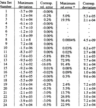
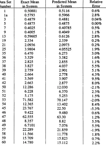
The analysis is based on the solution to a set of probability balance equations which approximate the average behavior of the link. We compare the new procedure
against exact numerical results, .and it is found to work well.
We also compare the approximate solutions obtained under the new procedure for
a single level of flow control against the approximation results obtained by using the
flow equivalent server approach, first applied to this problem by Avi-Itzhak and
ACKNOWLEDOrvtENTS
This research was supported by AIRMICS via the NCSU Center for
Communi-cations and Signal Processing, and by the Rome AirForce Development Center grant E-21-669-58 through the Georgia Institute of Technology. My deep thanks to these
organizations.
I also wish to acknowledge my indebtedness to Dr. 's Harry Perros and Salah
Elmaghraby. Both men have shown me every kindness and inspired me through their
TABLE OF CONTENTS
GLOSSARY OF SYMBOLS iv
1. wrR.ODUCfION 1
1.1 The Sliding Window Flow Control Environment 1
1.2 Problem to Address 12
1.3Definition of Symbols 16
2. UTERAT'UR.EREVIEW 19
3. THE LOWEST LEVEL MODEL 48
3.1 The Model 48
3.2 Maximum Throughput ofthe Model (Stability Condition) 54 3.3 Approximating the Throughput Characteristics ofthe Connection 57 3.4 AnAlgorithm for b00 ••••••••••••••••••••••••••••••••••••••••••••••••••••••••••••••••••••••••••••79
3.5 Approximation Results 84
3.6 Comparison to Flow Equivalent Server Technique 90
4. NESTED WINDOW FLOW CONTROLS 96
4.1The Model 99
4.2 Max.imum Throughput l 01
4.3 Approximation Procedure 103
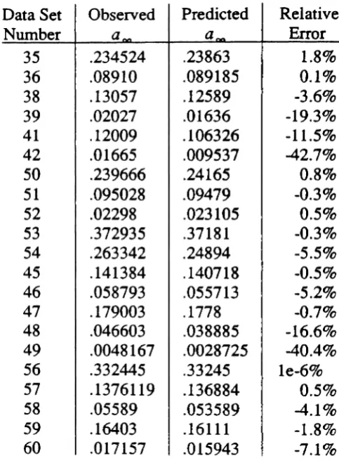
4.4 A Better Algorithm for
a
00 1194.5 Approximation Results 124
4.6 Multi-layer Simulation vs. Approximation Results 127 5. CONCLUSIONS AND SUGGESTIONS FOR FUTURE RESEARCH .133
REFERENCES 138
GLOSSARY OF SYMBOLS
In this glossary we define those symbols which are used in more than one Sec-tion of this thesis.
Symbol Definition Reference
Page
W window size
9
x
arrival rate 16B batch arrival size 16
f
number of transmission packets per high level packet.99
f
-1 is the maximum value ofnRPr( A } probability of event A
Pr( A I B } probability of event A given B
Jlx transmission time 48
J.LA acknowledgment time 48
1tw(W) Probability that two queue closed network of Figure 3.2, 54 page 55, has all tokens in the acknowledgment queue
1tw(W,yoo) As above when the transmission rate is replaced by 75
YooJlx
nA numberin acknowledgment queue 57
nT numberintoken queue 57
nx number in transmission queue 57
nH number in holding queue 57
ns
number of packets in system 57103 nR number of transmission packets in reassembly buffer 103
(i,j) state where
ns=i , nA
=1
57(i,j,k) state where
ns=i , nA
=1,
nR=k
103(jk ) state where nA
=1,
nR=k in closed network of Figure 110 4.4, page 102Pi,j probability of state(i,j) 58
Pi.jJc
-
probability of state (i,j,k) 103probability of
U
,k )for two models 110Yj,k'Yj,k
122
qi,j Pr{nH=i
,nT=1 }
30p.
I Pr{ns=i }
59P
n+1b·
,
Pr(nA
=W Ins=i }
59
-b an"average" b, 61
boo state asymptotic value of
b,
66r(yoo) an estimate ofboofrom (3.3.10) 76
a·I Pr(
nA
=W Ins=i }
in model of Figure 4.3 105a an "average"
a,
107The goal of this thesis is to present a methodology for predicting the perfor-mance of a computer communications link operating under a common type of
com-munications protocol known as sliding window flow control. We use this
introduc-tion to briefly describe the computer communicaintroduc-tions environment under study and to
introduce the terminology we will be using. We then describe the problem we wish
to solve, and indicate how succeeding Chapters address that problem.
As often as possible, we will use boldface type to highlight a term when it is
first used. The definition of the term can be found inthe surrounding text.
1.1. The Sliding Window FlowControl Environment
There are many issues which must be dealt with in the design of a data
com-munications network. Among these are how the data is to be organized, how to route
data through the network, how to encode the data electronically on the transmission
medium, and how to detect and recover from failure of the transmission medium to
transmit with 100% accuracy. Since all messages accepted to the computer network
must be stored, and buffer space is limited, the network designer must also find a way
to prevent or recover from users overloading the system.
In order to simplify the task of designing a data communications system, most systems are designed using a "layered" approach. The tasks which must be
hierarchical in nature; each layer provides a service to the layer above it, and receives service from the layer below it. While the services providedby each layer are well defined, the actual implementation of the service is hidden from the other layers. This allows layers designed separately to interact correctly as long as the interfaces
are agreed upon.
The layers accomplish their functions by exchanging data and messages with the same layerin another machine, using the lower layers to move the data and messages. We refer to the pair of communicating layers as
peers.
Each peer, of course, must be using the same conventions and definitions, referred to as the layerprotocol.
The peer to peer communication at a given layer is transparent to higher layer peers, which only see that the desired service is performed.highar
layers
lower
layers
Application
Presentation
Session
Transport
Network
Data- link
Physical
The transport layer is the highest layer of communications protocol. The
tran-sport peer at the sending end receives formatted data from the session layer, and uses
the lower layers to send that data to the receiving transport peer. The data units
han-dled by the transport layer are called messages. In many cases the lower layers, net-work, data link, and physical, are provided by a service not under the control of the
communicating host machines, as when one uses a public data network. The
tran-sport layer is thus often the lowest layer of communication protocol running in the hosts, and is designed to perform end to end communication functions relating to the
hosts.
A primary function of the transport layer is to prepare the session layer mes-sages for the network layer. Generally speaking, the amount of data that the session
layer peers exchange in anyone message is determined solely on the basis of
organi-zation of the data. For instance, in a file transfer application the session layer
mes-sage will be a file. The network layer, on the other hand, restricts the length of the
data units, called packets,that it handles. As we shall discuss in more depth shortly, a major function of the network layer is to avoid having too much work, (i.e. bits to be transmitted),in the network at any time. Having a maximum packet length allows the network layer to control the amount of work in the system by simply limiting the
number of packets accepted. It is the function of the transport layer to break the
arbi-trarily sized session layer message into the necessary number of network sized
pack-ets. The transport peer at the receiving host must be aware of this fragmentation and
session layer peer. Inthis way the session layer is isolated from the lower layer pro-tocols.
Another transport layer function is pacing. Either by agreeing on a data
transmission rate, or by explicit "send"f'don't send" messages, the communicating
transport peers limit how fast data issent to the receiver. This prevents a fast sender from giving a slow receiver more data than it can buffer.
A third transport layer function is error recovery. Some networks may destroy a
message in transit ifthe network becomes too congested. This may be done without notifying the sending transport peer. It is the responsibility of the transport layer to
decide that a message has been lost and to re-transmit it.
Another function which can be considered a transport layer function occurs in
the context of interconnected networks. We will return to this point after a discussion
of the network layer.
A computer network consists of a number of machines interconnected in some
fashion, so as to be able to exchange data. The network layeris responsible for rout-ing and flow control within a network. When the transport layer passes a message to
the network layer, broken up into one or more packets, the network layer must
deter-mine which sequence of transmission links in the network will be used to get those
packets to the receiver. Even if there is a directlinkthe network layer may decide to route the packets through some intermediate nodes to avoid congestion on the direct
As we mentioned previously, another means by which the network layer attempts to avoid congestion is by restricting the number of packets a given host may put into the network at any time. When there are too many packets in the network there may not be enough space in intermediate nodes to buffer all the traffic in transit through that' node. Queueing delays for transmission may also become excessive, leading to poor service for every network user, not just the users with a lot of traffic. When the network layer limits the number of packets a host has in the system, the network peer at the destination node must send a message back to the sending peer to notify it when more traffic can be allowed in. Inthe event that the number of packets allowed into the network is limited, this limit applies to network sized packets, and the sending transport peer is responsible for buffering any packets which cannot be allowed into the network: immediately.
number of packets allowed into the network. If the exit node should use all of its
available buffer space storing fragments of many different network packets, it would
not have any room to accept the completion of anyone of them. This problem is
referred to as reassembly deadlock.
There are two major classes of network protocols. The datagram protocols route each network packet independently, and packets can arrive in arbitrary order.
No guarantee of delivery is made in these protocols. The virtual-circuit protocols deliver packets in the order which they were transmitted. These protocols offer guaranteed delivery, and attempt to recover from lost packets.
The set of hosts known to a given network is not universal. Each network has
its own domain, although these may overlap. A machine which is connected to two
different networks and allows messages to be sent from one network to the other is
called a gateway. In the event that two machines which desire to conununicate are located on different networks, the transport layer peers are responsible for routing
messages from the sender's network to the receiver's network via gateways. In this case, the transport protocol is the only conununication protocol conunon to both
hosts, and the single transport connection will contain a concatenation of network
connections beneath it.
The complication of packet fragmentation also anses in an inter-network
environment. Different networks will have different maximum packet sizes. If a
message must go from a network with a given maximum packet size to one with a
entire message and then refragment it according to the new packet size, or fragment
each of the larger network's packets individually. In the latter case, the fragmented fragments could be reassembled either at the exit node of the network with the
smaller packet size or at the transport peer in the final destination.
(We note as an aside that some researchers reserve to the transport layer those
functions which run in the host machines only. Since inter-network routing requires
processing above the network layer at the gateways, these researchers define another
protocol layer, the inter-network layer, which lies between the transport and network
layers. Insome instances, such as the ISO inter-network standard, the inter-network layer may provide a flow control function).
Below the network layer is the data link layer. The data link layer is responsible
for monitoring the physical communication process. Each point-to-point link (hop) on the network is controlled by a data link layer; thus, in a network connection with
many hops, there will be many independent data link connections. Although each
hop has an independent data link connection and each could conceivably use a dif-ferent protocol, to the best of the author's knowledge of existing networks, within a
single network each data link connection uses the same protocol and maximum frame
size. (To have data link frame fragmentation between hops within a network would
introduce complications which no reasonable network designer would desire, and
thus the designers require that all nodes ina network use the same data link protocol). This means that there will be no fragmentation of data link frames between hops,
The primary function of the data link layer is to attempt to detect transmission
errors. In a typical data link protocol the receiving peer will check an incoming frame's checksum with that computed by the sending peer, and if the frame deter-mined to have transmission errors in it the receiver will either request that the sender
re-transmit that frame, Of, (as in the IEEE 802.x local area network standards), the
receiving data link peer will refrain from passing the faulty frame to the higher layer
peers, and depend upon the errOf recovery functions in the higher layers to cause a
re-transmission. If the frame is determined to be correct, an acknowledgment of
receipt is sent.
The data link peers also are responsible for managing the buffer space allocated
to them by their host machine. In order to prevent its buffer space from being filled
with traffic from a fast sender, the receiving data link peer can prohibit the sending
peer from transmitting frames temporarily, much as the transport peers do.
The lowest protocol layer, the physical layer, is concerned with the
representa-tion of data on the transmission medium. It is of no further interest tothis study.
A simple mechanism which is commonly used by designers to help achieve the
error recovery and flow control functions of the transport, inter-network, network,
and data link layers is a sliding window flow control. In a sliding window flow
con-trol the layer peers agree upon the maximum number of data units, (frames, packets,
or messages), which the sender may transmit without acknowledgment of correct
receipt. This maximum number is referred to as the window size of that connection.
In the remainder of this thesis, whenever we are discussing the behavior of a sliding window flow control protocol without specific reference to a protocol layer, we shall use the term packet to refer to the data units being exchanged, although strictly speaking the term packet is reserved to network layer data units. When we are specifically speaking of network layer packets, we shall make that clear.
In a connection using sliding window flow control, the sending peer numbers its outgoing packets with successive numbers from 0to W-1, and stores each one in its local buffer space. If the receiving peer finds that a packet isreceived incorrectly, a request to re-transmit is sent identifying the packet in error by its sequence number. When the receiving peer receives a correct packet, it sends an acknowledgement mes-sage to the sender, also indicating the sequence number of the correctly received packet. Upon receipt of an acknowledgment of correct reception, (or simply an acknowledgment), the sender can free up the buffer space holding that packet, use the newly freed buffers to accept a new packet, and reassign the sequence number to the new packet.
pro-tocols, a single acknowledgment message may be allowed to confirm correct receipt
of more than one packet. In this case, we view the acknowledgment as containing multiple tokens.
Let us see how sliding window flow control helps the different protocol layers
achieve their goals. The transport layer (and sometimes the data-link, network, and
inter-network layers) need to exchange information with their peers indicating
whether or not a transmitted packet was received correctly. Thisisinherent in sliding window flow control.
Sliding window flow control also protects the buffer space at the receiver, a goal
of each of the data link, network, and transport layers. The receiver has to buffer at
most W packets, and can delay sending an acknowledgment if its buffers are full.
Sliding window flow control also limits the buffer requirements of the sending node
in the data link layer. The sending data link peer only needs to keep a copy of the W
outstanding frames at any time, and can refuse to send acknowledgments to its
sendersifits buffers are full.
By limiting the number of packets outstanding on any connection, sliding
win-dow flow control helps the network layer limit the number of packets in the network. Packets waiting to get into the network must be stored by the network user, forcing
congestion outside the network boundary.
referred to the text by Tanenbaum, [Tane88]. An excellent discussion of the prob-lems in computer networks which mandate flow control, the paradigms used to address these problems, and actual network implementations of
flow
control schemes, including sliding window flow control, can be found in Gerla and Kleinrock, [Ger-Kle80].1.2. Problem to Address
In the previous section we introduced the concept of sliding window flow con-trol. The use of this mechanism, in some variant, is ubiquitous in protocol design. Sliding window flow control offers a convenient means of addressing some of the problems faced byprotocol designers, but it 'is not without its drawbacks.
acknowledgment arrives.
When the receiver is the slower process, occasional idleness at the sender when
there are packets available to transmit is not necessarily a concern. As long as a
token returns in time to allow the next packet to be transmitted and arrive at the
receiver before the receiver runs out of work, there will be no reductioninthe system throughput, Alas, it is the nature of sliding window flow control that this will not be
the case. Tokens returning in acknowledgments use the same transmission network as data packets, and are thus subject to unpredictable delays. In the worst case, we could have all of the tokens in acknowledgments making their way back to the sender, while the receiver is idle and the sender has packets to send. Inthis situation, no work is being done, even though both the sender and receiver are willing and able.
In light of the above discussion, we see that an important issue for network designers to consider is determining what exactly the throughput will be in a system
using sliding window flow control. It is this issue which we propose to address, at
least in part, in thisthesis.
To determine the throughput and other performance measures such as end to end
delay and buffer utilization in a network using sliding window flow control, requires an analysis which goes beyond application of the standard queueing network solution
techniques, such as the separability results of the BCMP theorem and the
approxima-tion algorithm of Marie, as there are features of the sliding window flow control
environment which violate the assumptions needed to apply these techniques. One
the above mentioned procedures is packet fragmentation and reassembly. Typical queueing network solving tools do not allow entities to split and re-coalesce. A second exceptional feature of sliding window flow control is the token/acknowledgment structure. The transmission server is forced to be idle when there are no tokens available. The frequency with whichthis happens depends upon the load on the system and the rate at which acknowledgments return to the sender, and is thus an integral part of the analysis. The existing general purpose techniques do not allow for the synchronization of two processes, transmission and acknowledg-ment, intheir formulation.
We will begin our investigation in Chapter 2 by reviewing the published litera-ture for modelling and solution techniques of sliding window flow controlled net-works.
Our goal in each of the models we consider is to reduce the given sliding win-dow flow controlled network, in which data packets and acknowledgments are
transmitted, to a flow-equivalent single server queue which handles only data
pack-ets. Acknowledgments do not appear in the approximation model. The service
characteristics of the server in the approximation model are calculated to reflect the degradation in data packet transmission capability caused by using sliding window flow control. We attempt to duplicate in the approximate queue the mean and distri-bution of transmission service time seen by data packets in the actual system, while keeping the characterization of the approximate server as simple as possible.
This approach allows us to replace a sliding window flow controlled
sub-network, which cannot be handled by standard queuing network analysis procedures,
by a single flow-equivalent queue which can be handled by these procedures. This effectively extends the class of networks which can be handled by the existing
tech-niques.
The approximation techniques can also be used to hierarchically analyze a link with multiple levels of sliding window flow control. Consider, for example, a link
with two levels of sliding window flow control. The higher level has as its delivery
mechanism a network which is a sliding window flow controlled network. The lower
level has as its delivery mechanism the physical link, which we represent as a single
server queue. Inthe hierarchical method we first reduce the lower level sliding win-dow flow controlled network to a single server queue. We then replace the lower
model now has a single queue as its delivery mechanism, rather than a sliding win-dow flow controlled network, and can be analyzed as the lower level was. Examples
and details of the hierarchical method are presentedin Chapters 2 and 4.
We conclude this thesis in Chapter 5 with a summary of the results and some reflections on possible extensions tothis research.
1.3. Definition of Symbols
We conclude this Chapter with a set of Figures introducing the symbols which
willbeused in this thesis.
Figure 1.2(a) is the symbol for a single server queue. We will indicate the
characteristics of the serverby anotation above the circle. A singleparameter, i.e.
Jl,
indicates exponential service time with rateJ.1.
An indexed parameter, i.e. J.1(n), indi-cates state dependent service with rate J.1(n) when there are n entities in the queue. E(J.1,k) indicates Erlang-k service with meanI/J.1.
The notation ,,-[B] in Figure 1.2(a)indicates that arrivals occur in batches of size B according to a Poisson process with mean rate
A.
Figure 1.2(b) will be used to represent the queue of available tokens at the
sender. A symbol above or below the queue represents the window size.
Figure 1.2(c) is a join symbol. Once an entity is present in each queue, they are
joined to form a single entity and released. This symbol is used to indicate assigning
a token to a packet. Figure 1.2(d) is a fork symbol. It represents the separation of
[6]
A
111111110
w
(0) -
queue and server
(b) - token queue11111111-+
1111111111-+
)
) )
)
(c) - A jo tn
(e) - fragmentat] on
(d) - A fork
(f) -
reassembly
Figure 1.2(e) is a fragmentation symbol. One entity entering on the left becomes n entities upon leaving. There is no delay associated with a fragmentation. Figure 1.2(t) is a reassembly symbol. Oncen fragments have arrived at this juncture, a single composite entity is released. There is no delay between the time the nth
CHAPTER 2 LITERATURE REVIEW
In this Chapter, we survey papers dealing with end to end window flow control which have appeared in the archival literature. We also survey selected papers from published conference proceedings, and two unpublished manuscripts.
Al
A2
L
J11
I
J12
AO - ")
~oT~oT
A
1 A2
•
• •
+~oMT
A M-l AM
(This is the well known "independence assumption", without which much analysis of computer communication networks would not exist). There is a limit ofW link
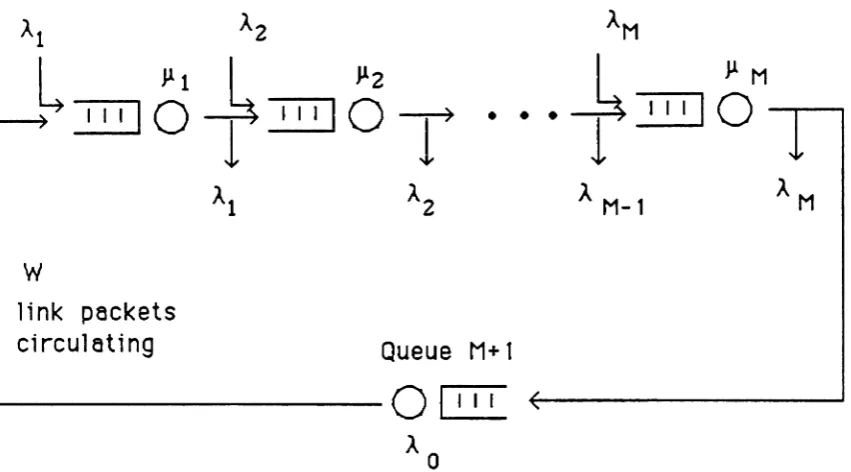
pack-ets allowed in the system at any point in time. There is no explicit acknowledgment mechanism in this model. Link arrivals which occur when there are already W link packets in the system are thrown away. Once there are fewer than W link packetsin the system, (once a link packet departs queue M), the next arrival will be accepted. Arrivals will continue to be accepted until the number of link packets in the system reaches W, at which point arriving packets are again rejected. This assumption we shall call the loss model assumption.
Under the loss model assumption we can represent the model of Figure 2.1 as
the closed network of Figure 2.2, with W link packets circulating. The closed
net-work has the same topology as the original, except that an additional queue, queue
M+ 1, is inserted after queue M and before queue 1. Service rate at queue M+ 1 is
Ao.
When allW link packets are in the transmission queues, (queues 1 through M), queue
M+ 1 is idle. When there are fewer than W link packets in the transmission queues, queue M+1 delivers link packets to queue 1 at rate
Ao.
We see then that queue M+1represents the link packet arrival process under the loss model assumption. Having
queue M+ 1be idle when all link packets are in transmission is the same as rejecting
arrivals which occur during this period.
The network of Figure 2.2, with link: packets using a closed network and
exter-nal arrivals seeing an open network, and having exponential servers at each queue,
A1 A2
L
J.l1
I
J.l2
~oT~oT
A
1
A
2•
•
A M-1 AM
W
1i
nk packets
ci rcul
at
ing
Queue
M+ 1"--- 0
~
A
o
external packets at each queue, from which other performance measures, (e.g.
transmission delay and system throughput), can be calculated. Ifwe denote by n, the
number of link packets in queue i, mi the number of external packets in queue i , i
=
1,2, · · · ,M, and let it and m be the vectors with components ni and mi,respec-tively, then the probability of the state (n,m ) is given by
__ M (n.+m.)' [
1.]
1Ii[A,.]
m,Pr{n,m}
=
Pr{O,O}n
r r ' _'''1)_ __ri=1 ni! m,!
J.li
J.li
Ifwe look only at the marginal distribution of link: packets, we have
M [
~
] 11;Pr(n} =G
n
A-t=1
J.1i -
i(2.1)
(2.2)
where G is a constant independent of
n.
The form of (2.2) is referred to as product form, since the probability of state if is a product ofM terms each involving only one value ofni' Thei'"
factor in (2.2) is proportional to the probability of havingnicustomers in an
MIMI!
queue with arrival rateAo
and service rate Ili-Ai; thus thestate probability of
it
has the form of the product of marginal distributions. We notealso that (2.2) is the solution of the closed network in Figure 2.2 with no external arrivals, and service rate at queue i of J.1'j =
J.li -
Ai' i.e., we can account for the external arrivals' effect on the distribution ofni simplybyreducing the service rate atqueue i by the external arrival rate at that queue! This technique has been referred to
as the method of adjusted rates, (see [Reis82]).
Chaterjee, Georganas, and Verma [ChGeVe77] extend the model of [penSch75]
routing, as opposed to a tandem configuration. This extension models a datagram
network protocol. As in the previous model, flow controlled packets arrive one at a
time according to a Poisson process, each transmission queue has Poisson external arrivals, the independence assumption is used, and the loss model assumption is
made. The original network under these conditions is represented as a closed net-work with an additional queue linking the netnet-work exit node(s) with the input
node(s). As before, this additional queue has service rate ~ and represents the
arrival process of link packets under the loss model assumption. With exponential
service rates at each queue, the joint probability distribution ofif and m has a form
verymuch like (2.1).
Martin Reiser [Reis79] presents a loss model of multiple independent sliding
window flow controlled connections sharing a communications network. (A similar
analysis appears in [LaPuMi79]). As in [penSch75] this model assumes that each of the R connections is a virtual circuit, and that its transmission path is thus a series of
queues. The independence assumption is used. Different connections have different
entry and exit nodes, and use a different sequence of transmission links, although
connections share some links. As in [penSch75] there is no explicit hop level flow
control in this model. The author assumes that the delays due to the datalink proto-col are incorporated into the link service time. Furthermore it is assumed that buffer
space at each transmission node is sufficient to ensure that no packets are rejected due
A source queue models the arrival process of packets for each connection. Asin [penSch75] the 'service rate of the source queue for connection r is the packet arrival
rate
A,.
of connection r. When all Wr tokens of connection r are in transit, the source queue for connectionr
is empty, and thus the arrival process quiesces.Acknowledgment packets are included in this model. It is assumed that the
acknowledgments use the same transmission path as the data packets, and the service
rate at each transmission link is reduced by the mean rate of work required to
transmit acknowledgments, (much as Pennotti and Schwanz account for external
arrivals in0(2.2». The acknowledgment path is then represented by a simple delay, the length of which is the average delivery delay along the transmission path. This approximation requires an iterative solution, as the average delivery delay is
influenced by the average number of tokens in the acknowledgment path, which in tumdepends upon the average delivery delay0 Acknowledgments are delivered to the
source queue, thus linking the output to the source.
As in the previous model, the loss model assumption reduces the network to a closed network. Inthis model the closed network has R classes of customers, one for each connection. Not surprisingly, this extension to the loss model occurred on the
heels of Reiser's development of an efficient algorithm for solving multi-class closed
queueing networks. This procedure, called mean value analysis, or MYA, is exactif the network has only B<:W> type stations, (see [BCMP75]). The major restriction of
used. Approximation procedures are presented which remove this restriction. A small test case validation is presented, and the approximation appears to be reason-able, particularly for predicting the throughput of each virtual circuit.
The loss models attempt to analyze a sliding window flow controlled networkby assuming that packets never queue for admission to the network. Another approach was taken by Kleinrock and Kermani [KleKer80]. These authors analyze a sliding window flow controlled network under saturation, that is, there is always a packet at the sending station when a token returns. This analysis also differs from the previous ones in that it explicitly models two features of sliding window flow control ignored in the previous models: message rejection at the destination node due to lack of buffers, and retransmissions by the sending station due to time-outs. A single con-nection is modelled, with no packet fragmentation. The analysis is modular; separate models are developed for the sending station, network, and destination node. The network is not modelled to any precision. It is simply assumed that both the transmission and acknowledgment delivery delays are exponentially distributed, with the same mean. Thus the round trip delay for a token has an Erlang-2 distribution. The probability of a time-out at the sending station can be calculated from this distri-bution and from the probability of having a packet rejected at the destination node.
re-transmissions), the probability of rejection can be calculated as the probability of an ~1/B queue having B customers in its queue. The equations for the probability of retransmission and the probability of destination node rejection both depend upon
the two unknowns, the rejection probability and the re-transmission probability. The
two equations are solved numerically for the estimates of these values.
Analysis of a sliding window flow controlled link under saturation can give
some idea of the maximum throughput achievable by the network, but is not useful for performance prediction under nonnalloads.
In his 1979 paper, Reiser indicates dissatisfaction with the loss model approach to analyzing sliding window flow control. A primary weakness ofthis analysis isthat it does not allow for true end to end delay prediction, since there is no means of evaluating the queueing delay which packets will incur waiting for a token.
It is also unclear how to set the rate A, in the queue which generates arrivals in these models. The true arrival rate
Ao
is not appropriate since the effective rate atwhich work enters the system is
A(
1 -Pr( source queue empty}). Reiser suggests solving the model using the true arrival rateAo,
getting an estimate of Pr{ sourcequeue empty}, and then re-solving the model with source server rate
A'
= -I-Prt source queue empty }This will allow the rate at which work enters the system to be closer to
A.a-
Of course in solving the model a second time a new value of the probability that the sourcerepeated until there is convergence.
While such an approach may be useful in raising the admitted traffic rate to the
true value, the mechanism of the source queue itself loses some of the flavor of
slid-ing window flow control, as every returning token in the loss model waits for a
packet, whereas in the actual system some tokens are used immediately by packets
enqueued for admission to the network.
In any event, the loss models are better than no analysis at all. Further progress in modelling sliding window flow control awaited further theoretical developments, which were not long incoming.
In 1981, Reiser [Reis8!] drew upon the flow equivalent server technique first presented by Avi-Itzhak and Heyman [AviHey73], to develop a model of sliding
win-dow flow control which includes admission delay. The model in this paper is of a single connection. Packets arrive one at a time according to a Poisson process to a
holding queue, (see Figure 2.3). IT there is a token available, the packet is paired with
the token, and the pair is delivered to the first transmission queue; otherwise, the packet waits in the holding queue for an acknowledgment. As.in [Reis79], the flow controlled connection is a multi-hop virtual circuit represented by a tandem
configuration. Service time is exponentially distributed at each queue, and the
independence assumption is used. There is no explicit modelling of hop level flow control; it is assumed that the delays due to this level of flow control are incorporated
into the link's service time. Packets are individually acknowledged. The
transmi
ss:
on queues
holding
queue
A~ ~ ~ V.1 V.z V. M
-7~O-7~O-~
• ••
~~O --7t~
-7~~
W
~token
queue
~--- ~~-_---I
<,acknowl edgment
delay
transmission delay is accounted for by reducing the service rate at the transmission queues.
Denote by nH the number of packets waiting for admission to the system, and by nr the number of tokens available at the sending station. W is the window size, and thus W -nT is the number of packets intransmission plus the number of acknow-ledgmentsin transmission.
The model is analyzed by replacing the transmission links and acknowledgment delay by a single queue with state dependent service rate 'j\W -nr). The resulting model is shown in Figure 2.4. We note that y(W-j) represents the rate at which tokens return to the token queue when
nr
=j, and thus the token round trip delay when nT = j is approximated by (W - j )/y(W -j). The mean data packet delivery delay when nT=
j is thus approximated by (W - j)/'j\W - j ) - ~, the mean round trip delay less the acknowledgment delay.The model of Figure 2.4 is fairly easy to analyze. Observing that nH and nT
cannotbesimultaneously non-zero, the system state probabilities
qi,j
=
Pr{ nH= i ,nT=j} obey the following steady state balance equationsAqo,w='j\l)QO,W-l
(A+y(W-j)qo,j ='j\W-(j-1»qO,j_l
+
Aqo,j+1 , j=W-1,W-2,···,1(A.
+
y(W»qo,o=AqO,I+
"«W)q1,0 (2.3)(A.
+
"«W »qi,0='j\W )qi+1,0+
Aqi-l,O, i=1,2,...,00W-n
T
In th1~ quaus
) )
'A
~IIIIIIII~~
qO,W-j = j qo,w ny(k)
k=1
qi.O= [
y(~)]
i qO.O', j=1,2,···,W
i=O,I, · · ·,00
w
ny(k)k=1
q
uw
is determined from the normalizationw
00'Lqo,j
+
'Lqi,O =1j~ ;=1
qo,w
The probabilities q;,j give a stochastic description of the model. Usingqi,j' y(j), and
~,performance measures can be calculated.
The crucial step in this method is calculation of the values y(j) ,j=1,2, . · · ,W. This is done using the so-called Norton's approximation server for the transmission network. (This name for the flow-equivalent server technique was coinedby Chandy, Herzog, and Woo [ChHeWo75], due to its similarity to the Norton's equivalent net-work theorem in electrical circuit analysis). Using this technique, y(j) is calculated by evaluating the closed network of Figure 2.5, which is the transmission and acknowledgment paths of Figure 2.3, "short-circuited". y(j) is set to the steady state throughput of the network in Figure 2.5 with j packets circulating. These values are
J.ll J.lZ
~O~~O-~
- - -
~+---a
j. packets
c
irc u
1atin g
new method to be superior. We note that the Norton's approximationanalysis can be just as easily applied to a datagram network, in which case the transmission network
is represented by a network of queues with random routing.
Thomasian and Bay [ThoBay84a] analyze a model with admission delays and
multiple virtual circuits. The approach is to generate a separate flow equivalent
server with state dependent service rates for each virtual circuit, using approximation
methods such as those in [Reis79] to estimate the network throughput characteristics
seen by each connection. This decomposes the model of R virtual circuits to R
models of the form of [Reis8!].
Oihr and Kuehn [OihKue85] extend the model of [ReisS!] by pointing out that
it can be used for fragmented arrivals to the holding queue by simply modifying the
balance equations (2.3) to the case of batch arrivals. (The modified balance equations
are presented in Section 3.6). This modifies the form of the solution for qi,j' but the method of analysis is the same. [GihKue85] is also of interest in that the transmis-sion server in their model is a single queue representation of a local area network.
The local area network was approximated by a single queue in a separate analysis.
This is an example of a hierarchical decomposition.
Varghese, Chou, and Nilsson [VaChNi83] analyzed the same network as in [Reis8!], but with zero acknowledgment delay. (The last queue in the tandem configuration can be viewed as the acknowledgment queue). These researchers found
that the Norton's approximation technique did not work very well, particularly when
representing the transmission network as a single queue with state dependent service
is presented, where the Norton's equivalent rate is used for nt
>
0, and a Coxian dis-tribution is used whennr
= O. The number of stages in the Coxian distribution is N, the number of hops in the transmission network. This technique was found to yield good results, but it is computationally intensive.Schwartz [Schw82] also draws upon the Norton's approximation technique in
his comparison of sliding window flow control with individual acknowledgments and IBM's SNA pacing control. The sliding window flow control model is the same
as
in [penSch75]. Extensive simulation experiments are reported on. Among the mostinteresting results are that the Norton's approximation does not work well withbulk arrivals, and that the independence assumption substantially underestimates the
throughput when the number of hops is larger than 3,particularly when the window size is small. The latter observation agrees with that of Varghese, et al,
([VaChNi83]).
Dallery [Dall87] presents a model of a sliding window flow controlled network
with admission delays which isbased on the analysis of a closed network model. The model in [Dall87] considers a transmission network with arbitrary topology, random
routing, and a general service time distribution at each station. The independence
assumption is used. There is no hop level flow control. A single connection is modelled. Packets arrive singly according to a Poisson process with mean
A
a and areacknowledged individually. Packets which arrive when there are no tokens available
Dallery analyzes a closed network consisting of the transmission stations from
the open network plus one additional station to represent the sending station. The
closed network has W tokens circulating. For a closed queueing network with
gen-eral service time distributions such as this, there are no fast exact algorithms like
MY A. Dallery uses a method due to Marie, [Mari79], which is an iterative numerical
approximation scheme for analyzing closed networks with general service time
distri-butions.
In Marie's method, each queue i in the network is analyzed in isolation, by
whatever technique is appropriate, for the probability of having ni customers in the
queue, (denoted Pi(ni
»,
assuming a state dependent arrival rateAi
(ni). These state dependent arrival rates are the throughput of the network with queue i removed,referred to as the complementary networkof queue i. Thus if there are W tokens in the system,
Ai
(ni) is evaluated by having W-ni tokens in the complementarynet-work of i. The result of the analysis for each queue i is a set of "conditional
throughputs",Vi
tn,),
which satisfy the equations(2.4)
The values Vi(ni) are used as state dependent exponential service rates at queue i
when analyzing the complementary network of some other queue j~i. Representing
each queue, regardless of its actual service time distribution, as a queue with state
dependent exponential service rate makes the analysis of the ~ relatively easy.
Marie's procedure is iterative. We initially begin with rough estimates of the
the
Aj
for other queues, and thus their conditional throughputs. This isturn changes theAi
values, thus we need to re-compute {Vi}again. The procedure continues until convergence is achieved.Let us denote the queue representing the sending station as queue T. We shall return in a moment to the values VT(i ) usedby Dallery in evaluating the closed net-work, but first let us look at how the solution of the closed network is used to deter-mine the behavior of the original open model.
After convergence of Marie's method, a set of valuesArU),j=O,l, · · ·,W,have been determined. These values are the state dependent rates at which tokens return to the sending station when there are j tokens in the token queue. Dallery then uses equations (2.3) from [Reis8l] to evaluate the sending station behavior, setting y(j) to Ar(W-j).
Now let us look at the values vT(i) used by Dallery. The conditional throughputs at the sending station queue should represent the delay tokens incur at the sending station. If there is more than one token at the sending station, then there can be no packets waiting, and thus the rate at which tokens will depart isthe arrival rate of packets,
A
a. This isthe same value of sending station service rate used in thesource queue of [Reis79] and [penSch75]. The analysis here differs in the condi-tional throughput assigned whennr=l. Inthis case, we use (2.4) to write
PT(O)
vT(l)=AT( 0 )
-PT(l)
esti-00
mates ofAr(W-j) for y(j). Pr(l)
=
qo,! andPr(O)= Lqi,O· The solution for vr(l)i=O
IS
[
VT(l)J1
-1=~
1 - Ar<O)1 (2.5)(2.5) is expressed in terms of the inverse of the conditional throughput, which is the expected delay, to illustrate that the expected delay at the source queue when nr=l is
less than the delay for an arrival to occur. Thus we see that the closed model to
approximate token behaviorin [Dall87] modifies the source queue behavior from that of [Reis79] and [penSch75] to account for the occasional fast departure of a token
from the sending station when it returns to find a packet waiting. Infact, (2.5) can be derived as the expected delay of a token at the sending station, conditioned upon it
arriving to anempty token queue.
We note that the values ofPr(O) andPr(l) used to determine vr(l) in (2.5) will change with each iteration of Marie's algorithm as the estimates of
Ar
U)
=y(W -j ) change.Dallery reports on comparisons of this procedure with simulation experiments.
The agreement is good. As with the other methods, the worst cases are when the
window size is small and the number of stations is large. We have already pointed
out that Marie's method is iterative, continually re-evaluating the conditional
throughputs and arrival rates until convergence occurs, and can thus be very
The paper by Fdida, Perros, and Wilk [FdPeWi87] is the only paper which we
shall survey which explicitly treats nested layers of sliding window flow control. The
paper presents an approximate solution methodology for a network with admission
delay. A single end to end connection is modelled, with no packet fragmentation. Packets are acknowledged individually. Each service station in the network is modelled as a queue and server. The independence assumptionisused. It is assumed that the servers are "BCMP-type", [BCMP75]. The significance ofthis last assump-tion will be discussed momentarily. Other than the restricassump-tion to BCMP-type servers,
the network between the sender and receiver allowed under this model isquite gen-eral. Parallel levels of flow-controlled networks can be placed in tandem, and levels of flow control may be nested. The transmission and acknowledgment networks are
assumed to be separate and independent, but the authors indicate how to removethis assumption.
The analysis of the systemishierarchical. At each step the lowest levels of flow controlled subnetworks are reduced to a single service station. These stations are
then used in the analysis of the next lowest level of flow control.
The reduction of a single flow controlled network is performed as follows.
Con-sider the flow controlled network of Figure 2.6. The arrival process to the holding
queue is assumed to be Poisson with rate
A.
The window size isW. Netl and Net2 are arbitrary networks of BCMP-type stations; Netl is the transmission network andNet2 is the acknowledgement network. Similar to [Reis8!], the behavior of the flow
net-holding
A.
queue
--+-1 I I .".,.".--~ --._~.
Net
1{Lnrj]
.~----.",.",..'
~-w '--
token
Queue
.
~-~ ---~.Net
2.~---- ~.
work formed by linking the outputs of Netl and Net2 to the inputs of Net2 and Netl, respectively, (see Figure 2.7). Call this new network Netl/2. Since by assumption both Net! and Net2 are composed of BCMP-type service stations, Netl/2 can be
easily analyzed exactly by the MVA algorithm. We perform the analysis of the closed network for each possible network population, 1,2,...,W, and for each popula-tionc we calculate two values,R'(c) andR" (c). R'(c) is the mean time to traverse
Netl when there are c packets in Net1l2, and R"(c) is the mean cycle time (time to traverse Netl and Net2) of Net 1/2 when there arec packetsin Netl/2. Define y(c ) as
c
IR"(c). y(c) is the rate at which customers leave Net2 when there are c packets in Net 1/2, i.e. nT=W-e. The original flow-controlled network of Figure 2.6 is now approximated by an infinite server queue with state dependent service rate R(c)givenby
'{R'(C),
c~W
R (c)
=
R'
(W)+
(c-W)/y(W),c
>WR(c) is an approximation to the mean time for a packet to traverse the original flow-controlled network when there are c packets in the system, (holding queue plus transmission network). For cS;W this time is approximated as R1
(c). For c>W a
packet must wait for (c -W) tokens to return to the sending station before it allowed into the transmission network. The approximation to this delay is (c-W)/y(W), where l/y(W) is the mean time for one token to return when there are W tokens in
Net 1
~---Net 2
Now let us examine how this technique is applied to nested levels of sliding window flow control. Consider the network of Figure 2.8, where S2 andS5 are slid-ing window flow controlled sub-networks, and Si- S3,S4' and S6 are general
net-works of BCMP type servers. Using the approach described above, S2 and S5 are replaced by single stations, each with a state dependent infinite server. Since such stations are BCMP stations, the transmission and acknowledgment paths of the approximate network are both networks of BC11P stations, and the reduction tech-nique is now applied to the new network.
Once we have hierarchically reduced all of the lower levels of flow control, the values y(j) are computed for the highest level model, and equations (2.3) are used to determine qi
.i .
Comparisons of this method against simulation results presented by the authors show that the method performs well. The accuracy declines as the utilization of the tokens increases.
The final paper we shall look at analyzes a sliding window flow controlled link in the context of HDLe, a common data...link layer protocol. The basic model analyzed by Labetoulle and Pujolle [LabPuj79] is shown in Figure 2.9. Packets arrive for transmission singly according to a Poisson process with rate
A.
Packets inA
-.. III
trsnsrm ss: on queue
1110
JJ.x
•
•
•
•
•
•
ecknowl edgment queue (1
nfi ni
te server))
rate f.1x. After transmission, packets go into an infinite server queue representing the acknowledgment mechanism. Packets leave this queue at the rate i
J.1A
when there arei packets in it. This state dependent service rate approximates the behavior of HDLe, where acknowledgment generally contain multiple tokens. This queueing model is solved approximately. The probability of having the acknowledgment queue full, (W packets), is estimated, and this is used to develop a service model of the transmission queue. The model of the transmission queue is evaluated for mean delays and queue lengths. No distribution results are obtained. Comparisons to simulation show the approximation to be quite good.
This method should prove useful as a sub-modelin approximations which incor-porate mean delay of data-link protocol in service time at a queue. Since the final service model of the transmission queue is rather complicated, this method may not be well suited for nested analysis.
We conclude this section with some remarks about related research areas which are not directly suitable for modelling sliding window flow control with admission delays.
Open queueing networks with population constraints have also been considered.
For two node queueing networks see [perr83] and the references within. Lam
[Lam77] considers multi-chain queueing networks with state dependent lost and
trig-gered arrivals. This paper extends the class of queueing networks which are known
to have a product form solution. Goto, Takehashi, and Hasegawa [GoTaHa83]
analyze an open tandem configuration with finite buffers and an overall population
constraint. All of these models ignore acknowledgment delays and use the loss
model assumption.
Two other related areas are the models of simultaneous resource possession and
serialization delays. These models either use closed network analysis, or are
specifically tailored to multiprogramming systems. For papers dealing with
simu-latneous resource possession see [perr8l], [JacLaz82], and [FreBex83]. Serialization
CHAPTER 3
THE LOWEST LEVEL MODEL
In this Chapter we present a model of a one hop single connection with sliding window flow control, and an algorithm for approximating its throughput and delay
characteristics.
3.1. The Model
The model under consideration is shown in Figure 3.1. Packets for transmission arrive in groups ofB to an infinite capacity holding queue at the sending station. The
arrival process is assumed to be Poisson with rate
A.
If a token is available at thetoken queue, then that token is paired with the first waiting packet in the holding queue and the token/packet pair is delivered to the transmission queue. This pairing
of tokens and packets and subsequent delivery to the transmission queue is assumed
to take place instantaneously, and continues until either the token queue or the
hold-ing queue becomes empty.
The packet/token pairs at the transmission queue are served one at a time in a first-come first-served fashion. Service times at the transmission queue are
exponen-tially distributed with a mean service time of l/Jlx. Upon completion of service at
the transmission queue, the packet leaves the system and the token is delivered
instantaneously to the acknowledgment queue. Tokens at this queue are served one
at a time, first-come-first-served, with an exponentially distributed service time of
mean l/JlA' Upon completion of service at the acknowledgment queue, the token is
[6]
holding
Queue
J1X
A
11111111-+
~~O~
)
)
II I 1I
II
I I 1-+
t ransmt ss
Queue
ion
token
W
Queue
J1
A
O~~
acknowl
edgment
Queue
with a packet. There are a total ofW tokens circulating in this model, W being the
window size of the flow control.
Let us discuss the features of this model as they relate to actual data
communi-cation systems. We assume that the arrival process is Poisson. Limited empirical
evidence suggests that this may indeed be the case in computer communication
environments, (see [Schw77]), as it is in telephony. In any event, queueing analysis is consideralbly more difficult without this assumption, and it is thus a common one
in communications modelling.
The holding queue represents the packets the higher layer has ready once the
modelled layer has a token available. The batch arrivals correspond to fragmentation
of the higher layer data unit.
We model the packet delivery mechanism as a single server queue with an
exponential service time distribution. In what follows we shall refer to the service
time in this queue as the transmission time, although there are other components to the delivery delay than just transmission. For instance, ifthere are other connections using the transmission channel, as will generally be the case, packets in the
connec-tion under study will suffer queueing delays while other connecconnec-tion's packets are
being transmitted, in addition to the queuing delays among packets of the connection
under study. We do not explicitly model other connections sharing the transmission
not model these delays here, but only assume that each packet is delivered correctly,
and that the time to delivery includes any required re-transmissions.
Our model also assumes that packets are delivered in the order in which they are
transmitted. This assumption is true in the case of virtual-circuit protocols, or
proto-cols which use a Itgo-back-n" scheme for re-transmissions. Althoughthis assumption
may be violated in some systems, throughput and buffer requirements will not be
affected" (as long as the time between packet deliveries regardless of order is exponentially distributed) since packets are assumed to be statistically identical;
how-ever, violation of this assumption will affect our delay analysis, in which we assume
that each packet must wait for delivery of each packet which arrived to the system
before it.
We do not explicitly model the time required for such protocol functions as
checksum computation, adding headers and trailers, and generating
acknowledg-ments. It can be assumed that the time for these functions is included in the delivery
time, but our model does not allow for these tasks to occur in parallel with the
transmission of another packet as is the actual case. The choice of whether to ignore
these protocol times or include them in the transmission time depends upon the
utili-zation of the system. If the system has a fairly high utiliutili-zation, much of the protocol
functions will be done while other packets are being transmitted. If packets typically
need to queue for transmission after protocol overhead functions are completed, then
we may as well ignore the time these functions take, since they are not the
server after protocol functions, as will be the case when the system islightly loaded, the inclusion of the protocol times in the delivery delay is appropriate. In any event, ifthe time for protocol functions is negligible with respect to the transmission time, either assumption will not severly affect the analysis.
To conclude, the assumption that the time between packet deliveries is
exponen-tially distributed is made without modelling many important features of actual data
communication systems. The decision not to explicitly model these features was
made to keep the model of focus as simple as possible. This decision is based on two
reasons. First, we wish to examine and evaluate the effects of sliding window flow
control protocols. The model to be considered, while idealized, can still give insight
into the effects of sliding window flow control. Secondly, we wish to examine a
model with as few analytical complications as possible at this point. Should we find
a successful approach for the simple model, it can point to means which may be
suc-cessful in more complicated models, as we will see in Chapter 4.
We also assume that the acknowledgments have an exponentially distributed
delivery time, but with a different mean than the data packets. The ratio of these
means, Jlx/J.lA' is a measure of the relative delivery times of the data packets and acknowledgments. If the ratio is much less than 1.0 this indicates that
acknowledg-ments return to the sender much more rapidly than data travels to the receiver. This
will be the case when data packets are large relative to the acknowledgments. When
the ratio is close to or greater than 1.0 this implies that either the data packets and
delays releasing acknowledgments. We do not model the receiver release delay and
acknowledgment transmission delay separately, but lump them together in the
acknowledgment server.
It is assumed that data packets are acknowledged one at a time. The situation in actual networks is more complicated; packets can be acknowledged in groups or
separately, even in the same protocol.
In our model the data packets and acknowledgments do not interfere with each other's transmission, despite sharing the same transmission network. In the case where acknowledgments have priority, it appears to the acknowledgments that there
is no interference from the data. In this case, the interference of the acknowledg-ments on the data transmission can be roughly accounted for by decreasing the data
transmission service rate proportionally to the amount of time required to transmit
acknowledgments. In networks where the acknowledgments do not have priority, we decrease both the acknowledgment service rate and the data transmission rate to
account for the time spent transmitting the other type of information. (See the
discus-sion of effective service rates in the review of [penSch75] in Chapter 2 for an exam-ple of this technique).
In sununary, our model is an idealized version of an actual sliding window flow
controlled connection, but retains the essential feature of such a connection, to wit,
transmission of data is suspended when all the tokens are in use. While the model as presented may be assailed for its simplifications, we note in partial defense that the
3.2. Maximum Throughput of the Model (Stability Condition)
One parameter of interest in looking at any queueing model is its maximum
throughput. This gives us an upper bound on the input traffic rate which the system
can handle. The boundis stated asan inequality, arrival rate
<
maximum throughput. Any arrival rate above the maximum throughput bound will result in anunstable sys-tem, so we wish to keep the input traffic below this bound.The maximum throughput can be evaluated by examining the system under
saturation. We posit an infinite queue of customers awaiting service by the system,
and observe the rate at which customers leave the system under this condition. This
rate is the maximum throughput.
This means of evaluating the maximum throughput is particularly easy for the
model of Section 3.1. With an infinite queue of packets waiting for transmission the
token queue becomes irrelevant, as each token returning to the sending station will
always find a packet waiting, and will thus immediately be used. The queueing
model for this situation is shown in Figure 3.2. The output of the acknowledgment
queue is connected to the input of the transmission queue, forming a closed network
of two exponential server queues withW tokens circulating.
Let us define
1ti(j) =Pr{ j tokens in ack. queue Ii tokens in model of Figure3.2 }. (3.2.1)
transm1
ss
ionqueue
JI.X
...--l.-.~O
W
tokens
circulating
J1 A acknowl
edgment
Queue
the acknowledgment queue the transmission server is delivering packets at the rate
Jlx. When all W tokens are in the acknowledgment queue the transmission server is idle, and thus has an effective service rate ofO. The closed system throughput is then
fJ.x(l-1tw(W»
+
O1tw
(W )=
fJ.x(l-1tw(W».All that remains to find the maximum throughput is to calculate 1tw(W). The
local steady state probability balance equations for 1tw(i) in the model of Figure 3.2
are
and a unique solution is obtained by using the normalizing sum
The solution to the above system of equations is
(3.2.2)
Thus
and the stability condition is