Optimal Control and Shape Design: Theory and Applications

(1)

LEWIS, BRIAN MATTHEW. Optimal Control and Shape Design: Theory and Ap-plications. (Under the direction of Hien T. Tran.)

This work focuses on the spectrum of problems connected with the analysis and the development of computational tools and models for engineering and scientific applications. This includes: (i) reduced order modeling techniques; (ii) linear and nonlinear feedback control design methodologies and real-time implementation; and (iii) shape optimization techniques. Excluding shape optimization techniques, most of the research herein can be seen as extensions of linear quadratic regulation (LQR) techniques. First, we consider the synthesis of control methodologies for the attenua-tion of beam vibraattenua-tions caused by a narrow-band exogenous force. By a narrow-band exogenous force we mean periodic force over a narrow frequency band or an exact harmonic. The control methods under consideration are based on the minimization of two specific quadratic cost functionals. One of these cost functionals is a typical time domain cost functional constrained by an affine plant. The other is a cost functional that is frequency dependent. These control methods have been used successfully in various applications but this investigation differs in that it emphasizes the develop-ment of real-time control methodologies based on reduced order models derived from physical first principles. Specifically, an integral component of this research is the proper orthogonal decomposition (POD) reduction technique and its application to real-time control of beam vibrations.

(2)

feedback controllers and state estimators for a broad class of nonlinear regulator prob-lems. The technique consists of using direct parameterization to bring the nonlinear system to a linear structure having state-dependent coefficient matrices. Then LQR techniques are used on the state-dependent coefficients to formulate a suboptimal control law. Theoretical advances have been made regarding the nonlinear regulator problem and the asymptotic stability properties of the system with full state feedback. However, there have not been any attempts at the theory regarding the asymptotic convergence of the estimator and the compensated system. This work addresses these two issues as well as discussing numerical methods for approximating the solution to the SDRE. A previous numerical method, which is based on the Taylor series, works only for a certain class of systems, namely with constant control coefficient matrices, and only in small regions. The interpolation numerical method, introduced here, can be applied globally to a much larger class of systems. Examples will be provided to illustrate the effectiveness and feasibility of the SDRE technique for the design of nonlinear compensator based feedback controllers.

Finally, this work also includes an optimization technique in which the objective is attained via alterations to the physical geometry of the system. This optimization framework, to be considered in the context of electron guns, is known as optimal shape design. Optimal shape design has been used in a number of applications in-cluding wing design, magnetic tape design, and nozzle design, among others. In this investigation, we use the methods of shape optimization to design the shape of the cathode of an electron gun. The dynamical equations modeling the electron particle path as well as the generalized shape optimization problem will be presented. Il-lustrative examples of the technique on gun designs that were previously limited to spherical cathodes will be given.

(3)

by

Brian M. Lewis

a dissertation submitted to the graduate faculty of north carolina state university

in partial fulfillment of the requirements for the degree of

doctor of philosophy

applied mathematics

raleigh, north carolina

June 2003

approved by:

H. T. Tran

chair of advisory committee

H. T. Banks

(4)

The author was born in Canton, Ohio on November 6th_{, 1976. He attended a small}

school in Malvern from kindergarten through graduation in 1995. During his junior and senior years of high school, he attended Kent State University, Stark Campus. After, he attended Morehead State University in Kentucky, graduating summa cum laude with a bachelor of science in mathematics with an area of concentration in computing. After a summer at Los Alamos National Laboratory, he came to North Carolina State University to study applied mathematics. He received his masters of science in applied mathematics in December 2000 and a doctor of philosophy in applied mathematics in May 2003. He has accepted a full time position at the Massachusetts Institute of Technology Lincoln Laboratory.

(5)

Many people deserve many thanks for their guidance and support. My advisor, Dr. H. T. Tran, has been a great teacher, mentor, and friend. Along with mathematical counsel he has provided insight into balancing work with nonacademic life. I thank Dr. K. Ito for his continued help and interest in my research, as well as for his interesting anecdotes. I would like to express my appreciation for the input and insight of Dr. H. T. Banks. I would also like to thank Dr. P. A. Gremaud and Dr. Z. Li who have both contributed time and effort to the completion of my dissertation. In addition, Dr. R. C. Smith has taken time to answer numerous questions about the beam project. Dr. W. M. McEneaney and Dr. R. H. Martin deserve many thanks also for the excellent classes in analysis and nonlinear control theory.

My deepest thanks go to the Center for Research in Scientific Computation and the Department of Mathematics for their continued financial support. Also, to Dr. T. M. Nguyen for the industrial opportunity at The Aerospace Corporation. In addition, thanks to Lawrence Ives and the rest of the engineers of Calabazas Creek Research, Inc. for all of the insight and financial support (through U.S. Department of Energy grant number DE-FG03-00ER82966).

This opportunity came into being due to the professors at Morehead State Uni-versity that encouraged me to attend graduate school. Dr. Seth, Dr. Boardman, Dr. Hammons, Dr. Spickler, Dr. Cyrus, Dr. Jaisingh, Dr. Malphrus, Dr. Nolan, Dr. Lindahl, and Randy Ross all helped me in some way or another in choosing my current path. Dr. Seth in particular suggested that I apply at N. C. State.

(6)

Dan, Bill, Jim, Pat, Katie, and Rob, have all made life entertaining. My parents, Ron and Patsy, have provided encouragement and support throughout my scholastic career and are the best of friends. Thanks also to my brother Tim and his family, Lynette and Callie, for being constant and fun. And lastly to my wife, Christina, thank you for being so understanding throughout this entire process.

(7)

List of Tables vii

List of Figures viii

1 Introduction 1

1.1 Introduction . . . 1

1.2 Objectives . . . 3

1.3 Linear Quadratic Regulator . . . 4

1.3.1 Full State Feedback . . . 4

1.3.2 LQR Based Estimation . . . 7

1.3.3 LQR Compensation . . . 9

1.4 Dissertation Outline . . . 10

2 Reduced Order Based Vibration Suppression 11 2.1 The Beam Model . . . 14

2.2 Estimation of Parameters . . . 33

2.3 Proper Orthogonal Decomposition Based Model Reduction . . . 40

2.4 Simulation of Open Dynamics . . . 50

2.5 Galerkin POD Error Estimates for the Euler-Bernoulli beam . . . 53

2.5.1 Numerical Extension to the Physical Beam . . . 78

2.6 Control Setup and Methodology . . . 85

2.6.1 Known Disturbance . . . 88

2.6.2 Frequency Shaped Feedback Control with Known Disturbance . . . 101

2.6.3 Frequency Shaped Feedback Control with Disturbance Estimation . . . 112

2.6.4 Robustness of Feedback Control . . . 116

2.7 Conclusions . . . 130

3 Nonlinear Control via the SDRE 131 3.1 Full State Response . . . 133

(8)

3.2.2 Interpolation Method . . . 152

3.2.3 Example 1 Revisited: Numerical Approximations . . . 154

3.2.4 5D Example . . . 160

3.2.5 3D Example . . . 161

3.3 Nonlinear Estimation . . . 167

3.3.1 State Estimator Example One . . . 173

3.3.2 State Estimator Example Two: Unstable Zero Equilibrium . . 174

3.4 Compensation Using the SDRE State Estimator . . . 177

3.4.1 Compensation Example . . . 187

4 Shape Optimization 190 4.1 Introduction . . . 190

4.2 Electron Gun Basic Elements . . . 191

4.3 Shape Optimization . . . 192

4.3.1 Nelder-Mead . . . 194

4.3.2 Implicit Filter . . . 196

4.3.3 DIRECT . . . 197

4.4 Shape Optimization of an Electron Gun . . . 198

5 Summary and Future Directions 213 5.1 Future Work . . . 215

List of References 217

(9)

2.1 Measured beam and patch parameters. . . 33

2.2 Parameter estimation, beam and patch parameters. . . 39

2.3 Parameter estimation cost functional values . . . 40

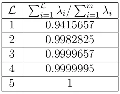
2.4 Energy contained in POD modes at 50 Hz. . . 49

2.5 Energy contained in POD modes at 20 Hz. . . 49

2.6 Energy contained in POD modes at 50 Hz with expanded ensemble. . 81

2.7 Control design parameters of Algorithm 2.2 used in real-time control of 50 Hz sinusoid. . . 97

2.11 Control design parameters of Algorithm 2.4 used in real-time control (with 3 POD modes) of 50 Hz sinusoid. . . 126

3.1 SDRE full state feedback: Comparison of Taylor series and interpola-tion SDRE numerical approximainterpola-tion methods . . . 157

3.2 SDRE full state feedback: Comparison of interpolation methods for 5D example . . . 161

4.1 Local results for optimal shape design withbd= 4.2 and bd= 4.4 . . . 206

4.2 Global results for optimal shape design withbd= 4.2 . . . 210

4.3 Global results for optimal shape design withbd= 4.4 . . . 212

(10)

2.1 Cantilever beam with piezoelectric patches. . . 15

2.2 Beam orientation (top view). . . 15

2.3 Cubic spline bases . . . 32

2.4 Transient parameter estimation results . . . 41

2.5 Periodic parameter estimation results . . . 42

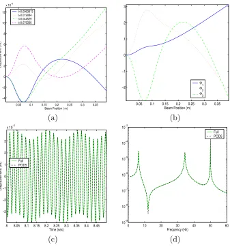
2.6 POD modes at 50 Hz . . . 50

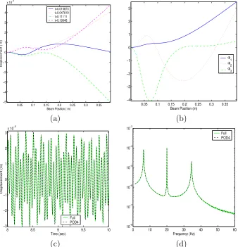
2.7 POD modes at 20 Hz . . . 51

2.8 Comparison of backward Euler and implicit trapezoid integration schemes 54 2.9 Comparison of implicit trapezoid, backward Euler, and central differ-ence integration schemes of full order dynamics . . . 80

2.10 Eigenvalues of the covariance matrices C1 and C2. . . 82

2.11 Comparison of implicit trapezoid, backward Euler, and central differ-ence integration schemes of POD reduced order dynamics . . . 83

2.12 Comparison of implicit trapezoid, backward Euler, and central differ-ence integration schemes of POD reduced order dynamics (same system matrices) . . . 84

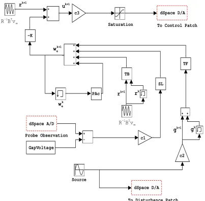
2.13 Flow chart for the cantilever beam test bed. . . 87

2.14 Cantilever beam photograph. . . 87

2.15 Known disturbance circular buffer . . . 90

2.16 Simulink for the known disturbance affine control law . . . 95

2.17 dSpace graphical user interface for known disturbance control. . . 96

2.18 Time series and FFT plots for known disturbance control . . . 99

2.19 Control and observer plots for known disturbance control . . . 100

2.20 Frequency shaping filter responses for different ξr . . . 102

2.21 Simulink for the frequency shaping control law (with full knowledge of the disturbance) . . . 107

2.22 dSpace graphical user interface for frequency shaping control (with full knowledge of the disturbance). . . 108

2.23 Time series and FFT plots for frequency shaping control (with full knowledge of the disturbance) . . . 110

2.24 Control and observer plots for frequency shaping control (with full knowledge of the disturbance) . . . 111

(11)

disturbance estimation). . . 118

2.27 Time series and FFT plots for frequency shaping control (with distur-bance estimation) . . . 119

2.28 Control and observer plots for frequency shaping control (with distur-bance estimation) . . . 120

2.29 Control results for frequency shaping (with disturbance estimation) when the roles of the patches are reversed . . . 122

2.30 20 Hertz Disturbance: time series and FFT plots for frequency shaping control (with disturbance estimation) . . . 124

2.31 20 Hertz Disturbance: control and observer plots for frequency shaping control (with disturbance estimation) . . . 125

2.32 Control results for frequency shaping (with disturbance estimation) when 3 POD modes are used . . . 127

2.33 Robustness result via table hit . . . 128

2.34 Robustness result via sinusoidal amplitude shift . . . 129

3.1 (a) Different values for G in Ge−βt _{and (b) plot of} _y _{(3.28) vs.} _x 1, y being negative (shaded) indicates region of attraction. . . 146

3.2 Full state feedback with exact SDRE solution close to the origin . . . 147

3.3 Full state feedback with exact SDRE solution away from the origin . 148 3.4 Eigenvalue comparison for SDRE exact and approximate closed loop matrices . . . 155

3.5 SDRE full state feedback: Comparison of Taylor series and interpola-tion methods for 2D example close to the origin . . . 158

3.6 SDRE full state feedback: Comparison of Taylor series and interpola-tion methods for 2D example away from the origin . . . 159

3.8 Continuity plots for toy example . . . 165

3.10 SDRE state estimator example: Stable zero equilibrium . . . 175

3.11 SDRE state estimator example: Unstable zero equilibrium . . . 178

3.12 SDRE compensator example . . . 189

4.1 Nomenclature associated with an electron gun. . . 193

4.2 The classic form for the steady Maxwell’s equations. . . 200

4.3 Free variables for the optimal shape design problem. . . 203

4.4 Flowchart for the local optimization routine. . . 206 4.5 Gun design with a spherical cathode and with the cathode initial guess 207

(12)

(13)

Introduction

1.1 Introduction

Accurate mathematical descriptions for complex physical systems and computational advances have allowed for a surge in the application of model based optimization and control theory to complex systems. Optimization routines that once took weeks to complete are now finishing in minutes and real-time control of complex systems, with the use of reduction, is becoming more achievable. Thus, there is an increasing demand for the development of theory and real-time results to justify the techniques that are becoming commonplace amongst engineers and mathematicians. Among the issues that one faces when designing model based control and optimization meth-ods are controller reduction, methmeth-ods for nonlinear control, and achieving optimality criteria of systems without using control (hence, achieving objectives through design). Controller reduction is of utmost importance in large scale control problems. For complex systems of partial differential equations (PDEs), the process of utilizing a real-time control involves approximation which can lead to large systems of ordinary differential equations (ODEs). There are a number of techniques to reduce the size of the system of ODEs that have received attention as of late including the proper orthogonal decomposition (POD), the modal approach, balanced realization and trun-cation, and LQG balancing and truncation. The first, POD, involves finding basis

(14)

functions that will represent the system in a better way than standard hat functions, cubic splines, etc., and then using the basis in the aforementioned approximation [20, 46, 41, 13]. Modal techniques use the natural modes (the eigenfunctions) of a structure to reduce the dimension of the system by eliminating the higher modes through a state transformation [24]. Balanced realization and truncation reduces the size of the controller using knowledge about the controllability and observability of the states [66]. The reduction is based on the magnitude of the Hankel singular val-ues. Hence, it is a transformation of the system matrices rather than reformulation of the system matrices using optimal bases. The last technique, LQG balancing and truncation [33], is a transformation based reduction technique similar to balanced realization and truncation. However, the system is reduced by examining the rela-tive size of the Riccati singular values so that the reduction is based on the control. Each of these reduction methods has strengths and weaknesses and must be tested for applicability.

(15)

its set of tuning rules that allow the modeler and designer to make trade-offs between control effort and output error. Other issues such as stability and robustness with re-spect to parameter uncertainties and system disturbances are also features that differ depending on the control methodology considered.

Model based control, either nonlinear or linear, is very useful in many situations. However, control usually involves some necessary physical elements, such as sensors and actuators, to observe the state and synthesize the control. Hence, it should also be of consideration as to when the objectives of the system can be met without the use of control. Rather, the system can be designed (geometry, mass balancing, etc.) with certain objectives in mind. Such analysis takes place in the fields of optimal shape design and free boundary problems.

1.2 Objectives

(16)

1.3 Linear Quadratic Regulator

Two of the three objectives that we have listed are directly related to linear quadratic regulation (LQR). Specifically, the attenuation of vibrations in the context of the cantilever beam will be achieved via simple extensions of LQR theory. Likewise, SDRE control can be seen as the nonlinear counterpart to LQR theory where the difference is that the system coefficient matrices are dependent on the state. Thus, since an understanding of LQR theory is important, we now present the background.

1.3.1 Full State Feedback

In this section, we assume that we have full knowledge of the state vector,x, and that the control objective is to find an input, u, that will result in asymptotic stability of the state dynamics. Here, the state dynamics are linear and are given by

˙

x=Ax+Bu, (1.1)

where x _{∈ <}n_, _u _{∈ <}m _, _A _{∈ <}n×n_{, and} _B _{∈ <}n×m_{. Associated with the state}

dynamics is the quadratic cost functional

J(x0, u) =

1 2

Z _∞

0

(xTQx+uTRu)dt, (1.2)

where Q _{∈ <}n×n _{is symmetric positive semidefinite (SPSD), and} _R _{∈ <}m×m _is

sym-metric positive definite (SPD). To find the optimal control (relative to the cost func-tional), we consider the Hamiltonian for this system which is given by

H(x, u, λ) = 1 2(x

T_Qx₊_uT_{Ru) +}_λT_(Ax₊_Bu), _(1.3)

where λ _∈ Rn _{is a Lagrange multiplier (that is also referred to as the co-state).}

(17)

satisfied:

Hx =−λ,˙ (1.4)

Hλ = ˙x, (1.5)

and

Hu = 0. (1.6)

Using (1.3), we have that the optimality criteria are then given by

˙

λ=₋Qx₋ATλ, (1.7)

˙

x=Ax+Bu, (1.8)

and

0 =Ru+Bλ (1.9)

for the LQR problem. From here, there are many ways to derive the algebraic Riccati equation (ARE) and to formulate the optimal control u. To be consistent with what is to be used for the state-dependent derivation, we opt to use the Sweep Method[43] and we assume that the co-state function λ is of the form

λ= Πx. (1.10)

The necessary conditions (1.7) and (1.9) become

˙

(18)

and

0 =Ru+BTΠx. (1.12)

Solving (1.12) for u, we obtain

u=₋R−1_BT_Πx. _(1.13)

Upon substitution of (1.13) into (1.8) we have that

˙

x= (A₋BR−1BTΠ)x. (1.14)

It is also true that ˙λ= Π ˙x= Π(Ax₋BR−1_BT_{Π)x. Setting this equal to (1.11), one}

finds

Π(A₋BR−1BTΠ)x=₋Qx₋ATΠx. This implies

Π(A₋BR−1BTΠ)x+ATΠx+Qx= 0, or

(ΠA+ATΠ₋ΠBR−1BTΠ +Q)x= 0. Since this is true for all x, it follows that

ΠA+ATΠ₋ΠBR−1BTΠ +Q= 0. (1.15)

Thus, the feedback control law is given by

(19)

To ensure asymptotic stability, conditions must be placed on the cost functional weighting parameters (Q and R) and the state and control coefficient matrices (A and B). This is summarized in the following theorem.

Theorem 1.1. Assume that(A, B)isstabilizable(meaning that for each state there

is a control that sends that state asymptotically to zero) and (A, Q1/2₎ _is _detectable

(all unobservable modes are stable), then the closed loop matrix A₋BK has

eigen-values with negative real parts and the system is asymptotically stable.

Proof. [1]

1.3.2 LQR Based Estimation

Full state feedback is quite often not realizable. This is due to a number of factors, including cost (of sensing equipment), efficiency, and reliability. Thus, it is necessary to estimate the state using output measurements. To formulate the estimator (also known as the observer), the case with no control effort is examined. The linear system, with output (y) and estimator (xe, also referred to as the state estimator), is given

by

˙

x=Ax, (1.17)

y=Cx, (1.18)

˙

xe=Axe+L(y−Cxe), (1.19)

where xe ∈ <n, y∈ <p, A∈ <n×n, and C ∈ <p×n. To show that the state estimator

converges to the actual state over time, the error

(20)

must be shown to converge to zero over time. Taking the derivative of (1.20) and using (1.17) and (1.19), we have the differential equation

˙

e=Ax₋Axe−L(y−Cxe). (1.21)

Since y=Cx, (1.21) becomes ˙

e= (A₋LC)e. (1.22)

It is well known that the solution to (1.22) is given by

e=e0exp((A−LC)t), (1.23)

wheree0 =e(0). IfL is chosen such that the constant matrixA−LC has eigenvalues

with negative real parts, the error will converge to zero asymptotically. Since the eigenvalues of the transpose of a matrix are the same as that of the original matrix, it is sufficient to find F =LT _{such that} _AT ₋_CT_F _{has all negative eigenvalues. An}

easy way to solve for F is to consider the dual LQR problem. Hence, we consider the cost functional

J(ˆx0,u) =ˆ 1₂R₀∞xˆTUxˆ+ ˆuTVu dtˆ (1.24)

with the dual dynamics given by

˙ˆ

x=ATxˆ+CTu,ˆ (1.25)

where U _{∈ <}n×n _{is SPSD and} _V _{∈ <}p×p _{is SPD. As shown in Section 1.3.1, the}

control law is given by

ˆ

u=₋Fx,ˆ where F =V−1_CΓ, _(1.26)

and Γ solves

(21)

The matrix A ₋C F has eigenvalues with negative real parts so long as (A , C ) is stabilizable (or (A,C) is detectable). Under this condition, the error converges to zero asymptotically and the observer gain is given by L= ΓCT_V−1_.

1.3.3 LQR Compensation

When all of the states are not available for feedback into the control, we use estimation techniques (as described in the previous section) to formulate the control u. The compensated system, using L and K as defined above, is given by

˙

x=Ax₋BKxe, (1.28)

y=Cx, (1.29)

˙

xe=Axe−BKxe+L(y−Cxe). (1.30)

The error dynamics are the same as in (1.21). In addition, the state dynamics are given by

˙

x=Ax₋BKxe+BKx(1−1)

= (A₋BK)x+BKe.

Thus, we find that the dynamics form the coupled system

 x˙

˙ e

 =



A−BK BK

0 A₋LC

 

 x

e



. (1.31)

(22)

1.4 Dissertation Outline

In Chapter 2 we consider the reduced order control of a cantilever beam. This work includes existence and uniqueness results for the Euler-Bernoulli beam with Kelvin-Voigt and viscous air damping as well as an error estimate for the POD reduced order dynamics integrated with a central difference type scheme. There are two control methodologies, one derived from the Hamiltonian in the time domain and one through frequency shaping techniques. We also consider two types of estimation, one in which it is assumed that full knowledge of the disturbance can be attained and one in which we assume that only the disturbance frequency is known. These estimation techniques are combined with the control methodologies to formulate three compensators: known disturbance; frequency shaping with full knowledge of the disturbance; and frequency shaping with disturbance estimation. Each of these compensators are implemented in real-time with full and reduced order systems.

The state-dependent Riccati equation technique for synthesis of nonlinear con-trollers and state estimators is presented in Chapter 3. We first review the basic derivation of the optimal control law using optimality criteria and then formulate the suboptimal control. We present a proof for full state feedback and the numerical methods currently available for approximation of the solution to the SDRE. We also consider the extension of the theory to estimation and compensation. We present theoretical results (local asymptotic convergence proofs) and numerical examples.

Chapter 4 is dedicated to geometrical shape optimization of electron beam guns. We present motivation as well as the general description of an electron gun. The dynamics and the tools available to simulate the particle pusher are also given. The optimization method employs the use of Nelder-Mead, implicit filter, and DIRECT algorithms so a short description of each is included. Optimization results are pre-sented for both local and global methods.

(23)

Reduced Order Based Vibration

Suppression

Piezoceramics, usually referred to as PZT materials or PZTs, are being used in various applications including acoustics, structures, and medicine. PZT materials exhibit electromechanical properties which can be utilized in actuator and/or sensor design. In particular, they enhance their physical dimensions when an electric voltage is applied to the material while a mechanical change in the dimension of the material induces a voltage difference across the material. This actuator/sensor duality classifies PZTs as smart materials. Structures that make use of these smart materials are known as smart structures. This investigation addresses, from a broad perspective, the feasibility of implementation of reduced order control methodologies for smart structures that make use of PZTs. In many situations, the object of the PZT smart material is to use its actuation capability to remove or minimize vibrations of the structure to which or in which it is molded or embedded.

In this work, we are concerned with an aluminum beam to which two PZT patches are mounted in a symmetric opposing fashion. The sensing device to be used for observation is a proximity probe and thus the sensor loading effects on the beam (an extremely thin metallic surface mounted on the beam) are assumed to be negligible and are not taken into account in the modeling of the beam. Also, it is assumed that

(24)

the beam vibration occurs transversely with no out of plane torsion or twisting about the axis of the beam. Thus, we are justified to make use of the Euler-Bernoulli beam model. We demonstrate these ideas in the context of a thin beam but the extension of analogous control techniques to more complex systems is straight forward.

(25)

The POD basis reduction method is becoming quite popular amongst control practitioners for decreasing the complexity and dimension of systems. This popularity of POD can be attributed to the method’s ability to accurately represent system data with a small number of basis elements. The POD method extracts characteristic system information from the data set via an orthogonalization process. The system data can be attained experimentally or by simulation of the system. POD has been used successfully in a variety of applications including turbulent coherent flows [4, 13, 12, 30, 44, 58], structures [49], and materials processing [37, 36, 45, 46, 62]. Furthermore, POD is found to be useful in the setting of feedback control, as found in [3, 2, 37, 36, 41]. In particular, the POD method has some history with the beam model that we are using and the CRSC beam. In [20], a POD reduced order observer was used to effectively control a transverse beam vibration due to transient pulsation utilizing LQR methodology. Our study differs in that we consider a more complex disturbance and we derive an error estimate for the use of POD in time integration, a task previously only accomplished in systems that are first order in time [42, 64].

(26)

2.1 The Beam Model

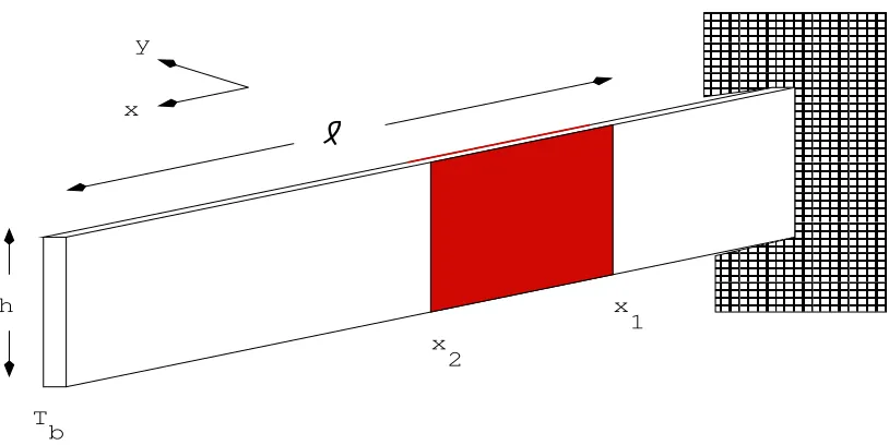
In this section we describe the partial differential equation (PDE) used to model the cantilever beam and an approximation to this PDE that is feasible for real-time com-pensation. To this end we consider a flat rectangular cantilevered beam, satisfying the Euler-Bernoulli (EB) displacement and Kelvin-Voigt (KV) damping hypotheses, to which piezoelectric patch actuators/sensors are mounted in a symmetric and opposing manner. Figure 2.1 is an illustration of this beam from the side while Figure 2.2 is the top view of the beam. As depicted, we impose a coordinate system with x-direction along the length of the beam and y-direction along the direction of transverse dis-placement. The end located atx= 0 is clamped while the end located atx=`is free. As depicted in the figure, the beam has dimensions: length `, width h, and thickness Tb. The patches are located between the points x1 and x2 and have a thickness of

Tp (not labelled in the figure). Further, the patches have the same width, h, as the

beam. As is necessary for the EB hypotheses, the beam has a constant cross section and is much smaller across than the length of the beam so that only small transverse displacement occurs and there is no torsion or twisting.

The transverse displacements y(t, x) of the beam, subjected only to forces and moments due to the patches and viscous air damping, are given by (see [8])

ρ(x)∂

2_y

∂t2 +γ

∂y ∂t +

∂2_M

∂x2 +

∂2_M

p

∂x2 = 0. (2.1)

The linear mass density, ρ(x), is piecewise constant due to the contribution of the patches and is given by

(27)

h

T b

x 2

x 1 y

x

Figure 2.1: Cantilever beam with piezoelectric patches.

+

-+v Back Patch

+v Front Patch

Proximity

Probe

(28)

where χ denotes the characteristic function given by

χ[x1,x2](x) =

  

1 if x_∈[x1, x2]

0 otherwise ,

and ρb and ρp are the volumetric mass density of the beam and patches, respectively.

We denote the viscous air damping parameter byγ so that the second term of (2.1), which is proportional to the transverse velocity, represents the air damping term. The internal moment is given by

M(t, x) =EI(x)∂

2_y

∂x2(t, x) +cDI(x)

∂3_y

∂x2_∂t(t, x) (2.2)

whereEI(x) is the Young’s modulus multiplied by the moment of inertia andCDI(x)

is the Kelvin-Voigt damping multiplied by the moment of inertia, both of which are piecewise constant due to the patches. These functions are given by

EI(x) =Eb

T3

bh

12 + 2h

3 Epa3χ[x1,x2](x) (2.3)

and

cDI(x) =cDb

T3

bh

12 + 2h

3 cDpa3χ[x1,x2](x), (2.4)

where, as before, the subscriptb represents the beam and the subscriptpdenotes the patch. Note that the moment of inertia for x /_∈[x1, x2] is given by

Ib =

Z Tb/2

−Tb/2

Z h/2

−h/2

ξ2dz dξ =h

Z Tb/2

−Tb/2

ξ2dξ= hT

3

b

12 (2.5)

while the moment of inertia for x_∈[x1, x2] is given by

Ib+2p =

Z Tb/2+Tp

−(Tb/2+Tp)

Z h/2

−h/2

ξ2dz dξ =h

Z Tb/2+Tp

−(Tb/2+Tp)

ξ2dξ = 2h(Tb/2 +Tp)

3

3 . (2.6)

(29)

for the patches so we subtract off (2.6) from (2.5) resulting in

Ip =

2h(Tb/2 +Tp)3

3 −

hT3

b

12 = 2h

3 a3, (2.7)

where

a3 = (Tb/2 +Tp)3−Tb3/8.

Finally, we have that the moment due to the patch is given by

Mp(t, x) =−Kχ[x1,x2](x) (V1(t)−V2(t)), where K=−

1

2Ephd31(Tb+Tp) (2.8)

and d31 is the piezoelectric strain parameter while V1 and V2 represent the voltages

applied to the front and back piezoelectric patches, respectively.

The cantilever beam has two boundary conditions at each end and initial condi-tions for both the displacement and velocity. At the fixed end,x= 0, the associated boundary conditions on the transverse displacement are

y(t,0) = ∂y

∂x(t,0) = 0. (2.9)

At the free end of the beam, x =`, the boundary conditions allow for free moment and shearing force and are given by

M(t, `) = ∂

∂xM(t, `) = 0. (2.10)

The initial conditions on the displacement and velocity are

y(0, x) = y0(x),

∂y

∂t(0, x) =y1(x). (2.11) For a detailed derivation of the beam model we refer the interested reader to [8].

(30)

that can lead to difficulties if finite difference methods are used to approximate the system. Therefore, to deal with this theoretically and computationally, we now con-sider the weak formulation for the beam. Letting ˙y:= ∂y_∂t and y0 _:= ∂y

∂x and dropping

dependence notation, equations (2.1) and (2.2) are rewritten as

ρ¨y+γy˙+M00+M_p00 = 0 (2.12)

and

M =EIy00+cDIy˙00. (2.13)

Upon multiplying (2.12) by a test function,φ, and integrating over the spatial domain we have

hρ¨y, φ_i_L2 +hγy, φ˙ i_L2 +hM00, φi_L2 =−

M_p00, φ®_L2. (2.14)

By requiring the necessary smoothness of y and ˙y, namely that they are in V = H2

L(0, `) = {φ ∈H2(0, `) | φ(0) =φ0(0) = 0}, and utilizing the boundary conditions

and integration by parts one arrives at (upon substitution of equation (2.13))

hρ¨y, φ_i_L2 +hEIy00, φ00i_L2 +hc_DIy˙00, φ00i_L2 +hγy, φ˙ i_L2

=_Kχ[x1,x2](V1−V2), φ

00®

L2,

(2.15)

where we have required that φ_∈V.

We now seek a solution to the weak form, a function y, with (y,y)˙ _∈V _×V, that satisfies (2.15) _∀φ _∈ V, for almost every t _∈ (0, tf) (tf some appropriately chosen

final time). The solution must also satisfy the boundary conditions (2.9) and (2.10) and the initial conditions for the displacement and velocity (2.11). We have that V ,_→ H ∼= H∗ _,_→ _V∗_{, thus forming a Gelfand triple with pivot space} _H ₌ _L2_{(0, `)}

where each embedding is continuous. This triple is endowed with a duality pairing

h·,_·i_V∗_,V defined by extending h·,·i_L2 on V ×H toV∗×H via continuity. Note that

(31)

forms σ1 :V ×V → <and σ2 :V ×V → <(we set<, the real numbers, as the range

space which is different than that considered in [8]) as

σ1(v1, v2) =hEIv100, v002i (2.16)

and

σ2(v1, v2) = hcDIv100, v200i+hγv1, v2i. (2.17)

Then, denoting

q(t) = _Kχ[x1,x2](V1−V2),

we have that equation (2.15) can be rewritten as

hρ¨y(t), φ_i+σ2( ˙y(t), φ) +σ1(y(t), φ) =hq(t), φi, (2.18)

with initial conditions

y(0, x) = y0(x) and ∂y_∂t(0, x) = y1(x), (2.19)

∀φ _∈ V, a.e. t _∈ (0, tf). If h·,·i is interpreted as h·,·iV∗_,V, then this is equivalent to

(2.12). From [8], under the assumption that y0 ∈ V, y1 ∈ H, and q ∈ L2(0, tf;V∗),

there exists a unique solutiony_∈L2_{(0, t}

f;V) to equation (2.18) with ˙y∈L2(0, tf;V)

and ¨y _∈ L2_{(0, t}

f;V∗). This solution depends continuously on the data (y0, y1, q).

For the sake of completeness we now present the theorem and proof for our specific system. For notational convenience in the proof, we define an equivalent weighted inner product forH =L2_{(0, `) as}

(32)

so that when φ _∈ H and ψ _∈ V then _hφ, ψ_iH = hρφ, ψiV∗_,V. Continuous embedding

of V inH implies that

(CE) For all φ_∈V, there exists a cV >0 such that kφkH ≤cVkφkV.

We now proceed to present the hypotheses for the theorem, starting with hypotheses onσ1:

(H1) (Symmetry) For allφ,ψ _∈V, σ1(φ, ψ) =σ1(ψ, φ).

(H2) (V-continuous) There exists a positive constant c1 such that for all φ, ψ ∈V

|σ1(φ, ψ)| ≤c1kφkVkψkV.

(H3) (V-elliptic) There exists a positive constant k1 such that for all φ∈V

σ1(φ, φ)≥k1kφk2V.

As can be seen, (2.16) adheres to these hypotheses. Since we have a specific damping term,σ2, we are able to make stronger assumptions than in [8]. Namely, we have that

σ2 satisfies

(H4) (V-continuous) There exists a positive constant c2 such that for all φ, ψ ∈V

|σ2(φ, ψ)| ≤c2kφkVkψkV.

(H5) (V-elliptic) There exists a positive constant k2 such that for all φ∈V

σ2(φ, φ)≥k2kφk2V.

It is evident that these hypotheses hold true for (2.17). Finally, we have that (H6) The input function q_∈L2_{(0, t}

(33)

We can now establish existence and uniqueness results for this system, where we have adapted Theorem 4.1 from [8] (and usedV2 =V).

Theorem 2.1. Suppose (H1)-(H6) hold true and thaty0 ∈V andy1 ∈H. Then there

exists a unique solution to y of (2.18) such that y_∈L2_{(0, t}

f;V), y˙ ∈L2(0, tf;V)and

¨

y _∈L2_{(0, t}

f;V∗). Additionally, solutions of (2.18) depend continuously on the data.

In other words, the map (y0, y1, q)→(y,y)˙ is continuous from V ×H×L2(0, tf;V∗)

to L2_{(0, t}

f;V)×L2(0, tf;V).

Proof. Let _{ξi}∞i=1 be a linearly independent total subset of V. Let us consider for

eachm a finite dimensional subspace ofV denoted byVm ₌_span_{_ξ

1, . . . , ξm}and for

eachm we let y0m, y1m ∈Vm be chosen so that y0m →y0 inV andy1m →y1 inH as

m_{→ ∞}. Let ym(t) =Pim=1ηim(t)ξi denote the unique solution to them dimensional

linear system

hy¨m(t), ξjiH +σ2( ˙ym(t), ξj) +σ1(ym(t), ξj) =hq(t), ξjiV∗_,V

ym(0) =y0m

˙

ym(0) =y1m,

(2.21)

for all j = 1, . . . , m. Then, for each j, we multiply (2.21) by ˙ηjm(t) and sum the

result over j to arrive at

hy¨m(t),y˙m(t)iH +σ2( ˙ym(t),y˙m(t)) +σ1(ym(t),y˙m(t)) = hq(t),y˙m(t)iV∗_,V. (2.22)

By (H1) we have that d

dtσ1(ym(t), ym(t)) = 2σ1(ym(t),y˙m(t))

and, upon multiplying each side of (2.22) by 2 and using this equality, (2.22) becomes d

dt

¡

ky˙m(t)k2H +σ1(ym(t), ym(t))

¢

(34)

We then integrate both sides from 0 to t to obtain

ky˙m(t)k2H +σ1(ym(t), ym(t)) + 2

Z t

0

σ2( ˙ym(s),y˙m(s))ds

=_ky˙m(0)kH2 +σ1(ym(0), ym(0)) + 2

Z t

0 h

q(s),y˙m(s)iV∗_,V ds

≤ ky˙m(0)k2H +σ1(ym(0), ym(0)) + 2

Z t

0 k

q(s)_kV∗ky˙_m(s)k_V ds.

We now make use of the fact that

0_≤(a₋2²b)2 =a2₋4²ab+ 4²2b2,

which is equivalent to

ab_≤ a

2

4² +²b

2_,

to obtain the inequality

kq(s)_kV∗ky˙_m(s)k_V ≤ 1

4²kq(s)k

2

V∗ +²ky˙m(s)k2V.

This, along with (H3) and (H5) leads to

ky˙m(t)k2H +k1kym(t)k2V + 2

Z t

0

(k2−²)ky˙m(s)k2V ds

≤ ky1mk2H +σ1(y0m, y0m) +

Z t

0

1

2²kq(s)kV∗ds.

(2.23)

Now, we fix ² so that δ = 2(k2 −²)>0 and note that since y0m → y0 and y1m →y1

inV then y0m and y1m are each bounded. Therefore, for sufficiently largem we have

that

ky˙m(t)k2H +k1kym(t)k2V +δ

Z t

0 k

˙

ym(s)k2V ds ≤M + 1

whereM =_ky1k2H+c1ky0k2V +

Rt

0 1

2²kq(s)kV∗ds.From this inequality, we can conclude

(35)

bounded. Therefore, because we have bounded sequences in reflexive spaces, there exists a subsequence of _{ym},{ymk}, and limit pointsy,yˆ∈L2(0, tf;V) such that

ymk * y inL2(0, tf;V)

and

˙

ymk *yˆin L2(0, tf;V).

We also have that for almost everyt_∈[0, tf), since ˙ymk(t) = Pmki=1η˙imk(t)ξi and ˙η are

almost everywhere bounded and continuous,

Z t

0

˙

ymk(s)ds = mk

X

i=1

µZ t

0

˙

ηimk(s)ds

¶

ξi

=

mk

X

i=1

(ηimk(t)−ηimk(0))ξi

=

mk

X

i=1

(ηimk(t)ξi)− mk

X

i=1

(ηimk(0)ξi)

=ymk(t)−ymk(0).

Thus,

ymk(t) = y0mk +

Z t

0

˙

ymk(s)ds (2.24)

in theV and, due to continuous embedding, H sense. By construction, we have that y(0) = y0mk →y0 in V. Also, since we know that ˙ymk *yˆ∈ L2(0, tf;V), it follows

that _Z

t

0

˙

ymk(s)*

Z t

0

ˆ y ds for each t _∈[0, tf). Thus, in the weak V sense we have

y(t) =y0+

Z t

0

ˆ y ds.

(36)

L2_{(0, t}

f;V).

To show that y is indeed a solution to (2.18) we return to the Galerkin equation (2.21). We consider a ψ(t)_∈C1_{[0, t}

f] with the terminal condition ψ(tf) = 0 and set

ψj(t) = ψ(t)ξj whereξj are as in (2.21). Then, upon fixingj < m, multiplying (2.21)

byψ(t), and integrating the result, we have

Z tf

0

½

hy¨m(s), ψj(s)iH +σ2( ˙ym(s), ψj(s)) +σ1(ym(s), ψj(s))

¾

ds

=

Z tf

0 h

q(s), ψj(s)iV∗_,V ds.

(2.25)

Using integration by parts and the terminal condition on ψ, we have that

Z tf

0 h

¨

ym(s), ψj(s)iHds = (hy˙m(s), ψj(s)iH)|tf₀ +

Z tf

0 h−

˙

ym(s),ψ˙j(s)iHds

=_−hy˙m(0), ψj(0)iH +

Z tf

0 h−

˙

ym(s),ψ˙j(s)iHds.

Substituting this back into (2.25) and rearranging, we see that

Z tf

0

½

h−y˙m(s),ψ˙j(s)iH +σ2( ˙ym(s), ψj(s)) +σ1(ym(s), ψj(s))

¾

ds

=_hy˙m(0), ψj(0)iH +

Z tf

0 h

(2.26)

We now use the fact that σ1(·, ψj(t)) and σ2(·, ψj(t)) are in V∗ for each t and the

weak convergence of ymk and ˙ymk to obtain, asm=mk → ∞,

Z tf

0

½

h−y(s),˙ ψ˙j(s)iH +σ2( ˙y(s), ψj(s)) +σ1(y(s), ψj(s))

¾

ds

=_hy1, ψj(0)iH +

Z tf

0 h

(2.27)

Recalling that ψj = ψ(t)ξj and further restricting ψ to have zero initial condition

(ψ _∈C∞

(37)

by parts and use of the initial and terminal conditions on ψ bring us to

Z tf

0

ψ(s) d

dshy(s), ξ˙ jiHds +

Z tf

0

ψ(s)

½

σ2( ˙y(s), ξj) +σ1(y(s), ξj)− hq(s), ξjiV∗_,V

¾

ds= 0.

(2.28)

But this implies that for each ξj

d

dthy(t), ξ˙ jiH +σ2( ˙y(t), ξj) +σ1(y(t), ξj) =hq(t), ξjiV∗,V. (2.29) Since _{ξk} is total in V we can conclude that ¨y ∈L2(0, tf;V∗) and (using (2.20)) for

all φ _∈V

hρ¨y(t), φ_iV∗_,V +σ₂( ˙y(t), φ) +σ₁(y(t), φ) =hq(t), φi_V∗_,V,

which is our desired result.

We already have that y(0) = y0. To show that ˙y(0) = y1 we return to (2.27)

and consider aψ(s) with zero terminal condition. Upon integrating the first term by parts, using the terminal constraint on ψ, and substitution of (2.25) we are left with

hy(0), ψ˙ j(0)iH =hy1, ψj(t)iH.

From this it follows that ˙y(0) =y1 and existence has been shown.

To show that the data is continuously dependent upon the initial conditions and q, we return to (2.23). From this inequality we see that

k_1kym(t)k2V +δ

Z t

0 k

˙

ym(s)k2V ds≤Km

where Km = ky1mk2H +c1ky0mk2V + 21²

Rt

0 kq(s)kV∗ds. Integrating over the interval

(0, tf) we have that

(38)

Taking limits and using weak convergence and lower semicontinuity of norms we see that

k_1ky_k2

L2₍₀_,tf_;_V₎+δt_fky˙k2_L2₍₀_,tf_;_V₎

≤tf

µ

ky1k2H +c1ky0k2V +

1 2²

Z t

0 k

q(s)_kV∗ds

¶

.

Finally, uniqueness is exhibited in the usual fashion by showing that the solution y_≡0 results only fromy0 =y1 =q= 0. We define for fixed, yet arbitrary, s∈(0, tf)

ψ(t) =

  

−Rtsy(ξ)dξ t < s

0 t _≥s ,

which implies ψ(tf) = 0. Using this as a test function in the weak form results in

hρ¨y(t), ψ(t)_iV∗_,V +σ₂( ˙y(t), ψ(t)) +σ₁(y(t), ψ(t)) = 0 (2.30)

and, since ˙ψ(t) = y(t) for almost everyt < s, we have

Z s

0

½

hρ¨y(t), ψ(t)_iV∗_,V +hρy(t), y(t)˙ i_V∗_,V

¾

dt =

Z s

0

d

dt{hρy(t), ψ(t)˙ iV∗,V} dt =_hρy(t), ψ(t)˙ _iV∗_,V|s

0 = 0.

Therefore we have that

Z s

0 h

ρ¨y(t), ψ(t)_iV∗_,V dt=−

Z s

0 h

ρy(t), y(t)˙ _iV∗_,V

and, upon integrating (2.30), we find

Z s

0 {h

(39)

We can then rewrite this (using (2.20)) as

Z s

0

d dt

©

ky(t)_k2_H ₋σ1(ψ(t), ψ(t))ª dt = 2

Z s

0

σ2( ˙y(t), ψ(t))dt. (2.31)

Since

d

dtσ2(y(t), ψ(t)) =σ2( ˙y(t), ψ(t)) +σ2(y(t), y(t)), we find (using ψ(s) =y(0) = 0)

Z s

0

σ2( ˙y(t), ψ(t))dt=

Z s

0

½

d

dtσ2(y(t), ψ(t))−σ2(y(t), y(t))

¾

dt =σ2(y(t), ψ(t))|s0−

Z s

0

σ2(y(t), y(t))dt

=₋

Z s

0

σ2(y(t), y(t))dt.

Thus, (2.31) becomes

ky(s)_k2_H +σ1(ψ(0), ψ(0)) =−2

Z s

0

σ2(y(t), y(t))dt (2.32)

and the use of (H3) and (H5) yields

ky(s)_k2_H +k1kψ(0)k2V ≤ −2k2

Z s

0 k

y(t)_k2_V dt. (2.33)

Since the right side is strictly negative it follows that

ky(t)_k2_H _≤0

which is the desired result.

(40)

(2.18). We make use of a subset of

S₃n_,B(0, `) =©ϕ _∈C2(0, `)_|ϕ is a cubic polynomial on [k`/n,(k+ 1)`/n]ª,

given by the following: For positive integer n, impose an extended uniform mesh along the beam length defined by _{xi}ni=+3−3, where xi = ih, h = _n`. On this mesh

define the spline basis _{sj}nj=+1−1 by

sj(x) =

1

h3

                          

(x₋xj−2)3, xj−2≤x≤xj−1

−3(x₋xj−1)3+ 3h(x−xj−1)2+ 3h2(x−xj−1)3+h3, xj−1≤x≤xj

−3(xj+1−x)3+ 3h(xj+1−x)2+ 3h2(xj+1−x)3+h3, xj ≤x≤xj+1

(xj+2−x)3, xj+1≤x≤xj+2

0, otherwise.

From this spline basis a modified basis that conforms to the boundary conditions at the clamped end, x= 0, is formed. This basis is _Bn₌_{_φ

j}nj=1+1 and is defined by

φj(x) =

    

−2s₋1(x) +s0(x)−2s1(x), j= 1

sj(x), 2≤j ≤n+ 1.

(2.34)

Since _Bn_{(0) = (}_Bn₎0_{(0) = 0, it is clear that} _span_{Bn_{} ⊂}_V_.

From the space span_{Bn_} _{we define a semi-discrete Galerkin approximation to}

the solution y of (2.18). Consider (2.18) restricted to span_{Bn_}_{, which is}

hy¨n_{(t), φ}_i

H +σ2( ˙yn(t), φ) +σ1(yn(t), φ) = hq(t), φi,

yn

0 =yn(0) =Qny0, y1n= ˙yn(0) =Qny1,

(2.35)

∀φ_∈span_{Bn_}_{, where}_Qn_{is the projection of}_V _onto_span_{Bn_}_{. Since this equation is}

(41)

with the form

yn(t) =

n+1

X

j=1

ηjn(t)φj, (2.36)

φj ∈ Bn. It is noted that due to finite dimensionality and linearity we need only

determine the ηjn(t) such that (2.35) holds for each φi ∈ Bn. To find these η, we

rewrite

˙ yn(t) =

n+1

X

j=1

˙ ηjn(t)φj

and

¨ yn(t) =

n+1

X

j=1

¨

ηjn(t)φj.

Upon substitution of these expressions into Equation (2.35), we arrive at (through the use of linearity)

n+1

X

j=1

¨

ηjnhρφj, φii_L2 +

n+1

X

j=1

˙

ηjnσ2(φj, φi) +

n+1

X

j=1

ηjnσ1(φj, φi) =hq(t), φii,

for i = 1, . . . ,(n + 1). Since the cantilever beam has symmetric opposing patches that are to be used for both disturbance and control, we letq(t) =χ[x1,x2](u(t)−g(t))

(whereu=V1 and g =V2). We are assuming that the control,u(t), and disturbance,

g(t), are distributed uniformly across the patch. Let

mij =hρφj, φii_L2, dij =σ2(φj, φi),

kij =σ1(φj, φi), and ˜Bi =χ[x1,x2], φi

®

L2,

(2.37)

i, j = 1, . . . , n+ 1. Furthermore, let ˜F = ₋B,˜ β = [η1n, . . . , η(n+1)n]T, M = [mij],

D= [dij], andK = [kij]. Under these definitions the system is rewritten as

Mβ(t) +¨ Dβ(t) +˙ Kβ(t) = ˜Bu(t) + ˜F g(t). (2.38)

(42)

If we are using the front patch for control and the back patch for distur-bance (which is the case for all but one of the results we present in the sequel),

˜

Bi =−χ[x1,x2], φi

®

and ˜F =₋B˜. This is depicted in Figure 2.2. Now, sinceyn

0 andyn1 are elements ofspan{Bn}, they have real vector representations

with respect to the φi, say β0 and β1, respectively. The right hand side is integrable

so this finite dimensional system has a unique solution on (0, tf). This means that

the η’s are uniquely determined and that they have all necessary regularity to ensure that the proposed solution yn_{(t) to (2.35) is correct. As discussed in [8], it can be}

shown that yn _→ _{y, where} _y _{is the unique solution to (2.18). Hence,} _yn _{is used, for}

sufficiently large n, as a model for the transverse vibrations of the beam described herein. We take n = 16. For the sake of implementation, we rewrite (2.38) in first order form as

˙

w(t) = Aw(t) +Bu(t) +F g(t), (2.39)

where

A=



 0 I

−M−1_K ₋_M−1_D

 ,

B =

  0

M−1_B˜

 , F =

  0

M−1_F˜

 ,

and w = [β,β]˙ T _with _w

0 = [β0, β1]T. Accompanying this ODE is the linear

displace-ment observation relation

wob =Cw,

where

C =hφ1(ˆx) . . . φn+1(ˆx) 01×(n+1)

i

(43)

For the reader interested in the computational aspect of creating these matrices, we note that the matrices (M,D, andK) are actually the sum of the beam and patch components. This is doable because we have symmetrically placed patches. Hence, we formulate Mb, Db, andKb whose elements are

mb

ij =hρbφj, φii_L2, db_ij =cDbIb

R`

0 φjφidx,

kb

ij =EbIb

R`

0 φjφidx,

and Mp, Dp, and Kp whose elements are

m_ijp =ρpR_xx₁2φjφidx, dpij =cDpIpR_xx₁2`φjφidx,

k_ijp =EpIp

Rx2

x1 φjφidx.

Then M =Mb+Mp, D=Db+Dp, and K =Kb +Kp.

To formulate the system matrices, we must use some form of numerical integration. The basis under consideration is a cubic spline basis so that the product of two basis elements is a sixth order polynomial. Thus, we are able to use a four point Gaussian quadrature rule to integrate exactly. The polynomials are defined piecewise which necessitates the use of integration over each subinterval (between neighboring nodes). Given that we are invoking a mesh withn points and step sizeh=`/n, we have that on thelth interval, [l₋1, l]_×h, the integration coefficientsci and quadrature points

xil are given by

c1 = ₆₍₁₈₊49√₃₀₎₂h, x1l = (l−1)h+h

·

1 2 −

√

15+2√30 2√35

¸

c2 = ₆₍₁₈₋49√₃₀₎₂h, x2l = (l−1)h+h

·

1 2 −

√

15−2√30 2√35

¸

c3 = ₆₍₁₈₋49√₃₀₎₂h, x3l = (l−1)h+h

·

1 2 +

√

15−2√30 2√35

¸

c4 = ₆₍₁₈₊49√₃₀₎₂h, x4l = (l−1)h+h

·

1 2 +

√

15+2√30 2√35

(44)

Therefore, the number of quadrature points is 4n. We then use two meshes, one over the entire beam to formulate Mb, Db, and Kb and one from x1 to x2 to create the

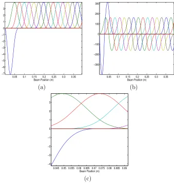
patch counterparts to these matrices, as well as ˜B and ˜F. As such, we must evaluate the cubic splines at each of the quadrature points. Figure 2.3(a) is a depiction of the splines at the quadrature points when n = 16 (note there are 17 modified splines) while Figure 2.3(b) is the derivative (note the conformity to the boundary conditions). Figure 2.3(c) is the splines evaluated over the patch quadrature points.

0.05 0.1 0.15 0.2 0.25 0.3 0.35

−7 −6 −5 −4 −3 −2 −1 0 1 2 3

Beam Position (m) 0.05 0.1 0.15 0.2 0.25 0.3 0.35

−300 −200 −100 0 100 200 300

Beam Position (m)

(a) (b)

0.045 0.05 0.055 0.06 0.065 0.07 0.075 0.08 0.085 0.09 −4

−3 −2 −1 0 1 2 3

Beam Position (m)

(c)

(45)

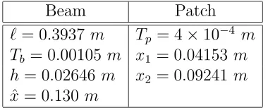
Beam Patch ` = 0.3937 m Tp = 4×10−4 m

Tb = 0.00105 m x1 = 0.04153 m

h= 0.02646m x2 = 0.09241 m

ˆ

x= 0.130 m

Table 2.1: Measured beam and patch parameters.

2.2 Estimation of Parameters

In the previous section we were able to use a Galerkin approximation to simplify the PDE (2.12) into a computationally feasible first order ODE (2.39). The hope then is to be able to accurately approximate the actual beam so long as modeling assumptions hold true and use the model to compensate the system. However, this model is incomplete until parameters are specified. The values that can be measured physically, `, h, Tb, Tp, x1, x2, and ˆx, are given in Table 2.1. Some of the other

parameters (ρb, Eb, ρp, Ep, and d31) can be obtained from the manufacturer but

these values are often averages and are disparate in particular scenarios. Moreover, because smart structures are composite structures, some of the parameters can un-dergo variations due to physical circumstances (epoxy, mount imperfections, material nonhomogeneities, etc.). Due to this, and the presence of parameters that cannot be measured (cD, cDp, and γ), an inverse or parameter estimation problem is

formu-lated for the parameters that are not directly measurable. The goal of the parameter estimation problem is to find a set of parameters so that the parameter dependent weak form closely resembles the actual physical system. For more information on the generic parameter estimation problem we refer the interested reader to [8]. For our particular problem we have the parameter dependent weak form given by

hρ(x;℘)¨y(t), φ_iL2 +σ₂(℘)( ˙y(t), φ) +σ₁(℘)(y(t), φ) =hq(t;℘), φi_V∗_,V,

y(0) =y0, y(0) =˙ y1,

(46)

for all φ_∈V, where℘ denotes the free parameters

℘=_{ρb, ρp, Eb, Ep, cDb, cDp, d31, γ} ∈P ⊂ <8,

and P is a set of admissible parameters. We are using displacement data collected with a proximity probe that is located at ˆx. Thus, we seek to find parameters so that when the model is evaluated at ˆx the solution is close to the data. One way of finding the optimal parameters is by using a least squares cost functional to compare the model to the physical data. Hence, a least squares cost functional that can be minimized over the parameter space, P, is

J1(℘, z) =

Nt

X

k=1

|y(tk,x;ˆ ℘)−zk|2, (2.41)

where zk is the kth observation from the proximity probe (corresponding to time

tk) and y(tk,x;ˆ ℘) is the beam model evaluated at ˆx on time tk with parameters ℘.

Since we are planning to use control methods that are based on accurate frequency information, we add a term to this functional to ensure accurate energy content of the model. Thus, the cost functional that we minimize to find the optimal parameters is

J2(℘, z) =

Nt

X

k=1

|y(tk,x;ˆ ℘)−zk|2+ 100 Nf

X

ζ=1

(fζ(y)−fζ(z))2, (2.42)

where fζ(y) is the ζth value of|FFT(y(t,x;ˆ ℘))| over alltk and fζ(z) is the ζth value

of _|FFT(z(t))_| over alltk. Here, we have denoted the fast Fourier transform as FFT.

As detailed in [8], we must consider a problem of feasible computational dimension and can accomplish this by using the Galerkin approximation (2.38) to estimate the infinite dimensional system dynamics. We can use this approximation because, if we define Qn _{as the orthogonal projection from} _H _onto_Sn

(47)

(A1) For each ψ _∈V we have

kψ₋Qnψ_kV →0

asn _{→ ∞}.

We define Hn _⊆ _V _{as the span of the set} _Bn _{(2.34). Since our parameter set is}

finite and it follows from the physical meaning of each of these parameters that P is bounded, we see that P is a compact subset of _<8_{. It follows that the hypotheses}

placed on σ1, (H1)-(H3), andσ2, (H4)-(H5), hold uniformly (independent of℘) on P.

If we define the metric d as

d(℘,℘) =˜

8

X

i=1

|℘i−℘˜i|

where℘1 =ρb, ˜℘1 = ˜ρb, etc., we see that these sesquilinear forms also conform to the

conditions

(H7) For all φ, ψ_∈V we have that

|σ1(℘)(φ, ψ)−σ1( ˜℘)(φ, ψ)| ≤γ1d(℘,℘)˜ kφkVkψkV.

(H8) For all φ, ψ_∈V we have that

|σ2(℘)(φ, ψ)−σ2( ˜℘)(φ, ψ)| ≤γ2d(℘,℘)˜ kφkVkψkV.

We will now give an argument for (H8) ((H7) follows similarly).

Proof. Recall that

σ2(φ, ψ) =

Z `

0

cDI(x)φ00ψ00dx+γ

Z `

0

φψ dx.

(48)

Then

|σ2(℘)(φ, ψ)−σ2( ˜℘)(φ, ψ)|

=

¯ ¯ ¯ ¯

Z `

0

(cDb −˜cDb)Ibφ00ψ00dx+

Z x2

x1

(cDp−˜cDp)Ipφ00ψ00dx

+(γ₋˜γ)

Z `

0

φψ dx

¯ ¯ ¯ ¯,

where the ˜_·are elements of ˜℘ and Ib and Ip are given by (2.5) and (2.7) respectively.

We then use the triangle inequality and the H¨older inequality resulting in

≤|cDb−c˜Db|Ib

µZ `

0

φ002dx

¶1/2µZ _`

0

ψ002dx

¶1/2

+_|cDp−˜cDp|Ip

µZ x2

x1

φ002dx

¶1/2µZ x2

x1

ψ002dx

¶1/2

+_|γ₋˜γ_|kφ_kL2kψk_L2.

By definition of the V = H2

L norm, kφkL2 ≤ kφk_V. We also know that opening up

the bounds on the “patch” integrals from (x1, x2) to (0, `) results in an inequality in

the right direction. Finally, since

µZ `

0

φ002dx

¶1/2

=¡_kφ00_k2_L2

¢1/2

≤¡kφ_k2_L2 +kφ0k2_L2 +kφ00k2_L2

¢1/2

=_kφ_kV,

we have (with γ2 = max{Ib, Ip,1})

≤γ2(|cDb−˜cDb|+|cDp−c˜Dp|+|γ−γ˜|)kφkVkψkV

≤γ2d(℘,℘)˜ kφkVkψkV.

(49)

Theorem 2.2. Suppose that H _⊆ V for all n and (A1) holds. Assume that the

sesquilinear forms σ1(℘) andσ2(℘)satisfy (H1)-(H5) uniformly, as well as (H7) and

(H8). Furthermore, we assume that the map

℘ _→q(_·;℘)

is continuous from P to L2_{(0, t}

f;V). Then, asn → ∞ we have

yn(t;℘)_→y(t, ℘)

and

˙

yn(t;℘)_→y(t, ℘)˙

in V for almost every t > 0. Here, y is the solution to (2.40) and yn _{is the solution}

to the finite dimensional Galerkin approximation given by

hρ(x;℘)¨yn_{(t), φ}_i

L2 +σ₂(℘)( ˙yn(t), φ) +σ₁(℘)(yn(t), φ) =hq(t;℘), φi

yn_{(0) =}_Qn_y

0, y˙n(0) =Qny1.

(2.43)

Proof. see [8]

To solve the inverse problem we made use of two data sets. We chose to use two data sets so as to avoid local minima with the Nelder-Mead numerical optimization algorithm (see Chapter 4). The first data set, ztr_{, was generated by a 125.6 volt}

transient pulse (a narrow triangular shaped voltage estimating an impulse function) sent to the front patch of the beam. The second data set, denoted zωd_{, is from a}

(50)

an implicit trapezoid scheme detailed in the sequel. We also found that the initial condition (the displacement and velocity) could not be set to zero. As can be seen in Figure 2.4(a) and (c) there is some sort of disturbance (either from the light, computer monitor, etc.) that is exciting the beam before the transient pulse (which occurs at approximately 0.49s). Thus, to approximate the initial condition, we use a model based observer for 0.15 seconds (the shaded region in the figures). Once this time period has passed, we then integrate the model dynamics for the remainder of the 2 seconds using the displacements and velocities of the observer at t = 0.15 for the initial condition of the model.

As mentioned, a Nelder-Mead search algorithm is used to vary the parameters of the finite dimensional model in an attempt to find a minimum to the parameter estimation problem. Since we are using two sets of data, we seek to minimize

J_sn(℘, ztr, zωd) =J_trn(℘, ztr) +J_ωdn(℘, zωd) (2.44)

where Jn

tr is the finite dimensional version of (2.42) using a transient source for the

model, yn

tr, given by

J_trn(℘, z) =

Nt

X

k=1

¯

¯yn_tr(tk,x;ˆ ℘)−ztrk

¯ ¯2

+ 100

Nf

X

ζ=1

¡

fζ(ytrn)−fζ(ztr)¢

2

, (2.45)

and Jn

ωd is the finite dimensional version of (2.42) using a periodic source with a

magnitude of 125.6 volts for the model, yn

ωd, given by

J_ωdn(℘, z) =

Nt

X

k=1

¯

¯y_ωdn (tk,x;ˆ ℘)−z_kωd

¯ ¯2

+ 100

Nf

X

ζ=1

¡

fζ(yωdn )−fζ(zωd)¢

2

. (2.46)

In both cases we denote fζ(yn) as the ζth value of |FFT(yn(t,x;ˆ ℘))| over all tk and

fζ(z) as theζth value of|FFT(z(t))| over alltk (wherez is eitherztr orzωd, etc.). As

(51)

Book Values Estimate ρb (kg/m3) 2.7×103 2.5354×103

ρp (kg/m3) 7.7×103 3.8462×103

Eb (N/m3) 6.9×1010 6.4670×1010

Ep (N/m3) 5.5×1010 2.7370×1010

cDb (N s/m2) (6.9×105) 7.4030×105

cDp (N s/m2) (5.5×105) 2.1412×107

d31 (m/V) −179×10−12 −364.03×10−12

γ (N s/m2₎ _(0.01) _1.6254_×₁₀−2

Table 2.2: Parameter estimation, beam and patch parameters.

modified cubic splines is 17 and the dimension of the system is 34. This number was chosen because we obtain sufficient convergence and we are limited in dimension for real-time implementation. Table 2.2 lists the parameters that have been estimated via the inverse problem (ρb, ρp,Eb,Ep,cDb,cDp,d31, andγ) and their respective book

values, if available. The numbers enclosed in parenthesis are for the parameters for which we have no book values. As such, the values in parenthesis are those that we use for the initial guesses in the optimization. As evidenced in the table, some of the optimized parameters are quite different than the given book values. For instance, the optimizedd31value is almost double the book value. We attribute this to a number of

(52)

Data IGFV OPTFV Transient 1.5355_×10−5 _1.3265_×₁₀−7

Periodic 4.9692_×10−5 _1.1773_×₁₀−6

Sum 6.5047_×10−5 _1.31_×₁₀−6

Table 2.3: Cost functional values, IGFV = the initial guess functional value, and OPTFV = the optimal functional value.

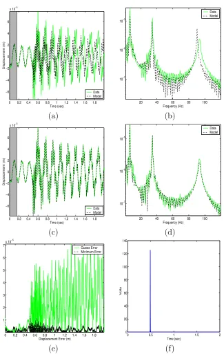
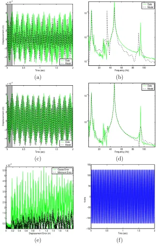
the displacements of the measured probe data and the model with optimal values for the transient pulse while Figure 2.4(d) is the frequency content. As can be seen from the plots, the model using the estimated parameters nearly matches the measured data. The displacement error over time is given in Figure 2.4(e) as well as the source in Figure 2.4(f). Figure 2.5 gives the same plots for the sinusoidal source. Finally, in Table 2.3 we provide the functional values for the transient data (2.45), the periodic data (2.46), and the sum of the transient and periodic data (2.44) (the decision criteria in the optimization).

2.3 Proper Orthogonal Decomposition Based

Model Reduction

(53)

0 0.2 0.4 0.6 0.8 1 1.2 1.4 1.6 1.8 −6 −4 −2 0 2 4 6

x 10−5

Time (sec)

Displacement (m)

Data Model

20 40 60 80 100 10−7 10−6 10−5 Frequency (Hz) Data Model (a) (b)

0 0.2 0.4 0.6 0.8 1 1.2 1.4 1.6 1.8 −6 −4 −2 0 2 4 6

x 10−5

Time (sec)

Displacement (m)

Data Model

20 40 60 80 100 10−7 10−6 10−5 Frequency (Hz) Data Model (c) (d)

0 0.2 0.4 0.6 0.8 1 1.2 1.4 1.6 1.8 1 2 3 4 5 6 7x 10

−5

Displacement Error (m)

Guess Error Minimum Error

0 0.5 1 1.5 2

0 20 40 60 80 100 120 140 Time (sec) Volts (e) (f)

Figure 2.4: Transient source plots for parameter estimation, (a) time series data and model with book param-eters, (b) absolute value of the FFT of data and model with book paramparam-eters, (c) time series data and model with

optimized parameters, (d) absolute value of the FFT of data and model with optimized parameters, (e) absolute error

(54)

0 0.5 1 1.5 2 −6 −4 −2 0 2 4 6 8x 10

−5

Time (sec)

Displacement (m)

Data Model

20 40 60 80 100 10−7 10−6 10−5 Frequency (Hz) Data Model (a) (b)

0 0.5 1 1.5 2

−6 −4 −2 0 2 4 6 8x 10

−5

Time (sec)

Displacement (m)

Data Model

20 40 60 80 100 10−6 10−5 Frequency (Hz) Data Model (c) (d)

0 0.2 0.4 0.6 0.8 1 1.2 1.4 1.6 1.8 0.5 1 1.5 2 2.5 3 3.5 4 4.5 5 5.5

x 10−5

Displacement Error (m)

Guess Error Minimum Error

0 0.5 1 1.5 2

−150 −100 −50 0 50 100 150 Time (sec) Volts (e) (f)

Figure 2.5: Sinusoid source (with 31.5 Hz frequency) plots for parameter estimation, (a) time series data and model with book parameters, (b) absolute value of the FFT of data and model with book parameters, (c) time

series data and model with optimized parameters, (d) absolute value of the FFT of data and model with optimized

parameters, (e) absolute error between data and model with book values and data and model with optimized values,