Analysis and Optimization of Speed, Feed and
Number of Teeth of Circular Saw for a Special
Purpose Sawing Machine
A. H. Rasal1, Prof. (Dr.) V. R. Naik2, R. A. Mane3
M.E. P.D.D. Student, Department of Mechanical, Textile and Engg. Institute, Ichalkaranji, Kolhapur,
Maharashtra, India.1
Head of Mechanical Department, Textile and Engg. Institute, Ichalkaranji, Kolhapur, Maharashtra, India.2
Asst. manager, Paranjape Autocast Pvt, Ltd,,Satara, Maharashtra, India.3
ABSTRACT: This paper deals with the increasing of productivity by selecting suitable machining parameters i.e.
speed, feed and number of teeth, of a special purpose machine designed and developed for sawing process. The component is a cylinder head made of aluminium alloy (IS designation 4223).This machine uses a carbide tipped circular saw. The feeding of job against the circular saw is done hydraulically. The tests are conducted and reading are tabulated using MINITAB software. Response Surface Methodology technique is used for analysis and optimization of the mentioned parameters.
KEYWORDS: Response Surface Methodology, speed, feed, number of teeth Surface roughness, Production rate.
1. INTRODUCTION
In industry, designed experiments can be used to systematically investigate the process or product variables that influence product quality. After identifying the process conditions and product components that influence product quality, direct the improvement efforts to enhance a product's manufacturability, reliability, quality, and field performance.
Because resources are limited, it is very important to get the most information from each experiment to be performed. Well-designed experiments can produce significantly more information and often require fewer runs than haphazard or unplanned experiments. In addition, a well-designed experiment will ensure evaluation of the effects identified as important. For example, if there is an interaction between two input variables, be sure to include both variables in the design rather than doing a "one factor at a time" experiment. An interaction occurs when the effect of one input variable is influenced by the level of another input variable. Designed experiments are often carried out in four phases: planning, screening (also called process characterization), optimization, and verification [1].
II. RELATED WORK
Response surface methodology (RSM) uses various statistical, graphical, and mathematical techniques to develop, improve or optimize a process. Response surface methods are used to examine the relationship between one or more response variables and a set of quantitative experimental variables or factors. These methods are often employed after identifying the controllable factors and find the factor settings that optimize the response. Designs of this type are usually chosen when there is a curvature in the response surface.
iii. Identify new operating conditions that produce demonstrated improvement in product quality over the quality achieved by current conditions
iv. Model a relationship between the quantitative factors and the response
Process parameters
Cutting speed (rev / min): It is a travel of a point on the cutting edge relative to the surface of cut in unit time in the process accomplishing the primary cutting motion. It is expressed in rev/min [2,3].
Cutting feed (mm / sec): The work table on which the component is mounted advances towards the circular saw with the specified feed. It is expressed in mm/sec.
Number of teeth: Circular saws have specified number of teeth. These are available according to the company manufacturing catalogue [4].
Response parameters
Surface roughness (µ): It is component of surface texture. It is qualified by vertical deviations of real surface from its ideal form. Unit is micrometer.
Production rate: The total number of components machined in a specified time limit. It can be specified as jobs / hour or jobs / shift or jobs / day.
III. DESIGN OF EXPERIMENT
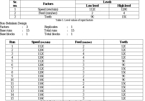
The design of experiment (D.O.E.) chosen for the special purpose machine is a Response surface methodology, by carrying out a total number of 15 experiments [5]. According to the manufacturing catalogues, range of process parameters is selected as mentioned in following table. The number of teeth for circular saw is selected as per standard.
Sr.
no. Factors
Levels
Low level High level
1 Speed (rev/min) 1120 1200
2 Feed (mm/sec) 2 4
3 Teeth 90 150
Table 1: Level values of input factors
Box-Behnken Design
Factors : 3 Replicates : 1
Base runs : 15 Total runs : 15
Base blocks : 1 Total blocks : 1
Run Speed (rev/min) Feed (mm/sec) Teeth
1 1120 2 120
2 1200 2 120
3 1120 4 120
4 1200 4 120
5 1120 3 90
6 1200 3 90
7 1120 3 150
8 1200 3 150
9 1160 2 90
10 1160 4 90
11 1160 2 150
12 1160 4 150
13 1160 3 120
14 1160 3 120
15 1160 3 120
The above table shows the combination set generated for each single run [6-8]. These combinations are set accordingly and tests are conducted. The worker used is same individual during the total testing procedure.
IV. EXPERIMENTAL INVESTIGATION
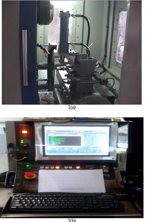
The following image shows the designed and developed special purpose machine. Fig 1(a) shows the set up of cutting mechanism that mainly includes carbide tipped circular saw, a fixture using hydraulic clamp system for holding the job. Fig 1(b) shows the control panel used for adjusting the process parameters such as cutting speed & cutting feed. Its values are seen on the display monitor.
1(a)
1(b)
Fig 1: (a) Image of the special purpose machine (b) Image of the control panel.
V. EXPERIMENTAL RESULT
Run Speed
(rev/min) Feed (mm/sec) Teeth
Surface roughness
(µ) Production rate
1 1120 2 120 1.312 855
2 1200 2 120 1.415 872
3 1120 4 120 1.391 868
4 1200 4 120 1.495 898
5 1120 3 90 1.437 868
6 1200 3 90 1.561 882
7 1120 3 150 1.269 872
8 1200 3 150 1.321 885
9 1160 2 90 1.392 868
10 1160 4 90 1.597 884
11 1160 2 150 1.325 875
12 1160 4 150 1.415 893
13 1160 3 120 1.495 888
14 1160 3 120 1.395 872
15 1160 3 120 1.425 878
Table 3: Runwise values of surface roughness and production rate
VI. ANALYSIS USING RSM
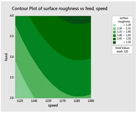
Analysis of response surface roughness: The following Fig 2(a) shows the contour plots generated for surface
roughness versus speed, feed . This helps to verify the value of surface roughness obtained for corresponding values of speed & feed. Fig. 2(b) shows a graphical representation of obtained surface roughness values for a specified set of speed, feed, & number of teeth.
2(b)
Fig 2: (a) Contour plot of surface roughness (b) Main effects plot for surface roughness
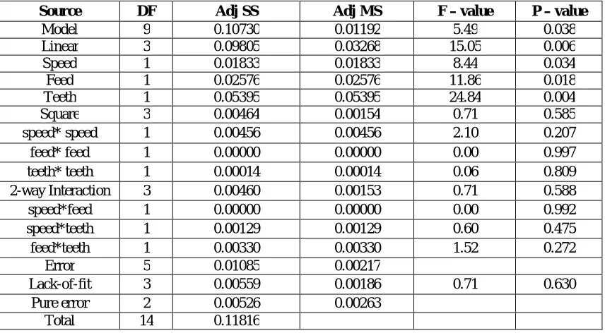
The table 4 represents analysis of variation of the process parameters for surface roughness conducted through the software. It also shows the corresponding F-value & P-value which are within the permissible range.
Source DF Adj SS Adj MS F – value P – value
Model 9 0.10730 0.01192 5.49 0.038
Linear 3 0.09805 0.03268 15.05 0.006
Speed 1 0.01833 0.01833 8.44 0.034
Feed 1 0.02576 0.02576 11.86 0.018
Teeth 1 0.05395 0.05395 24.84 0.004
Square 3 0.00464 0.00154 0.71 0.585
speed* speed 1 0.00456 0.00456 2.10 0.207
feed* feed 1 0.00000 0.00000 0.00 0.997
teeth* teeth 1 0.00014 0.00014 0.06 0.809
2-way Interaction 3 0.00460 0.00153 0.71 0.588
speed*feed 1 0.00000 0.00000 0.00 0.992
speed*teeth 1 0.00129 0.00129 0.60 0.475
feed*teeth 1 0.00330 0.00330 1.52 0.272
Error 5 0.01085 0.00217
Lack-of-fit 3 0.00559 0.00186 0.71 0.630
Pure error 2 0.00526 0.00263
Total 14 0.11816
Table 4: Analysis of variation for surface roughness
Term Effect Coef SE Coef T – value P – value VIF
Constant 1.4383 0.0269 53.46 0.000
Speed 0.0958 0.0479 0.0165 2.91 0.034 1.00
Feed 0.1135 0.0568 0.0165 3.44 0.018 1.00
Teeth -0.1642 -0.0821 0.0165 -4.98 0.004 1.00
Speed* speed -0.0703 -0.0352 0.0243 -1.45 0.207 1.01
Feed* feed 0.0002 0.0001 0.0243 0.00 0.997 1.01
Teeth* teeth -0.0123 -0.0062 0.0243 -0.25 0.809 1.01
Speed* feed 0.0005 0.0003 0.0233 0.01 0.992 1.00
Speed* teeth -0.0360 -0.0180 0.0233 -0.77 0.475 1.00
Feed* teeth -0.0575 -0.0287 0.0233 -1.23 0.272 1.00
Table 5: Coded coefficients for surface roughness.
Regression equation in uncoded units
Surface roughness = -31.9 + 0.0540 speed + 0.164 feed + 0.0192 teeth - 0.000022 speed*speed + 0.0001 0.000007 teeth*teeth + 0.000006 speed*feed- 0.000015 speed*teeth - 0.000958 feed*teeth
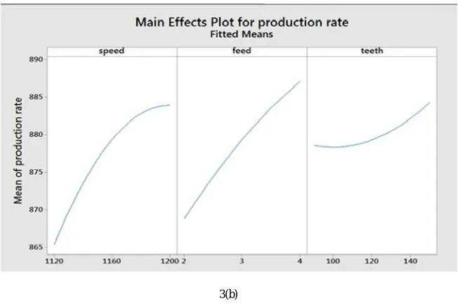
Analysis of response production rate: The following Fig 3(a) shows the contour plots generated for production rate
versus speed, feed. . This helps to verify the value of production rate obtained for corresponding values of speed & feed. Fig. 3(b) shows a graphical representation of obtained production rate values i.e. the total number of components machined within the specified time span, for a specified set of speed, feed, & number of teeth.
3(b)
Fig 3: (a) Contour plot of production rate (b) Main effects plot for production rate
The table 6 represents analysis of variation of the process parameters for production rate conducted through the software. It also shows the corresponding F-value & P-value which are within the permissible range.
Source DF Adj SS Adj MS F – value P – value
Model 9 1568.48 174.276 4.49 0.056
Linear 3 1416.75 472.250 12.1 0.01
Speed 1 684.50 684.500 17.6 0.00
Feed 1 666.13 666.125 17.1 0.00
Teeth 1 66.13 66.125 1.70 0.24
Square 3 108.23 36.078 0.93 0.49
speed* speed 1 80.41 80.410 2.07 0.20
feed* feed 1 7.41 7.410 0.19 0.68
teeth* teeth 1 16.03 16.026 0.41 0.54
2-way Interaction 3 43.50 14.500 0.37 0.77
speed* feed 1 42.25 42.250 1.09 0.34
speed* teeth 1 0.25 0.250 0.01 0.93
feed* teeth 1 1.00 1.000 0.03 0.87
Error 5 193.92 38.783
Lack-of-fit 3 63.25 21.083 0.32 0.81
Pure error 2 130.67 65.333
Total 14 1762.4
Table 6: Analysis of variation for production rate
Term Effect Coef SE Coef T – value P – value VIF
Const-ant 879 3.6 244 0.00
Speed 18.5 9.25 2.2 4.20 0.008 1.0
Feed 18.2 9.13 2.2 4.14 0.009 1.0
Teeth 5.75 2.88 2.2 1.31 0.248 1.0
Speed*speed -9.33 -4.67 3.2 -1.44 0.209 1.0
Feed* feed -2.83 -1.42 3.2 -0.44 0.680 1.0
Teeth* teeth 4.17 2.08 3.2 0.64 0.549 1.0
Speed* feed 6.50 3.25 3.1 1.04 0.344 1.0
Speed* teeth -0.50 -0.25 3.1 -0.08 0.939 1.0
Feed* teeth -0.0575 0.50 3.1 0.16 0.879 1.0
Table 7: Coded coefficients for production rate.
Regression equation in uncoded units
Production rate = -3072 + 6.78 speed - 78.6 feed - 0.27 teeth - 0.00292 speed*speed - 1.42 feed*feed + 0.00231 teeth*teeth + 0.0812 speed*feed - 0.00021 speed*teeth + 0.017 feed*teeth
4(a)
4(b)
The above Fig 4 (a) represent the surface curve generated for various values of surface roughness with respect to the different combinations of the process parameters whereas Fig 4 (b) represent the surface curve generated for various values of production rate with respect to the different combinations of the process parameters. Through this graph, set of process parameters can be selected for desired values of surface roughness and production rate.
VII. OPTIMIZATION USING RESPONSE SURFACE METHODOLOGY
The following figure shows optimum parameters set of speed, feed and number of teeth which give relevant response values of surface roughness and production rate. This graph shows the predicted values for low, medium and high values of surface roughness and production rate. It focuses on the overall effect of the process parameters on each output parameters. The highlighted lines and values shows the values of speed, feed and number of teeth required for obtaining optimum values of surface roughness and production rate.
Fig.5: Multi Optimization plot using RSM
VIII. CONCLUSION
The following conclusions can be drawn ,
1.As the cutting speed increases from 1120 rpm to about approximately 1180 rpm, the surface roughness increases gradually form points 1.350 to 1.450. After 1180 rpm, the surface roughness becomes steady and eventually decreases then after.
2.As the feed increases, the surface roughness goes on increasing gradually.
3.As the number of teeth goes on increasing, the surface roughness is highly affected. For maximum number of teeth on circular saw, the surface roughness obtained is minimum.
4.As the speed increases, the production rate also increases. After the speed of 1180 rpm, the production rate remains steady up to a certain limit.
5.As the feed increases, the production rate increases gradually. For maximum feed, maximum production rate is obtained and vice versa.
6.The number of teeth on circular saw from 120 to 140 help to increase the production rate.
Thus the solution is as,
The following multi optimization result table shows the final values of the process parameters to achieve minimum surface roughness and maximum production rate.
Input parameters Output parameters
Speed (rev/ min)
Feed
(mm/ sec) No. of Teeth Surface roughness (µ)
Production rate (components / shift)
1200 3.798 150 1.36 898
REFERENCES
[1] Aman Aggarwal and Hari Singh, Optimization of machining techniques, A retrospective and literature review Optimization on machining techniques, Vol. 30, Part 6, pp.: 699–711, December 2005.
[2] Basim A. Khidhir and Bashir Mohamed, Study of cutting speed on surface roughnessand chip formation when machining nickel-based alloy, Journal of Mechanical Science andTechnology, Vol 24, Issue 5, pp :1053-1059,2010.
[3] J. Kovak, M. Mikles, Research On Individual Parameters For Cutting Power Of Woodcutting Process By Circular Saws, Journal Of Forest Science, Vol. 56, pp.: 271 – 277, 2010.
[4] Jan Svoren, The Analysis Of The Effect Of Number Of Teeth Of Circular Saw Blade On Critical Rotation Speed, Acta Facultatis Technicae,
Vol. 17, pp.: 109 – 117, 2012.
[5] John Allen, Dragos Axinte, Paul Roberts, Ralph Anderson, A review of recent developments in the design of special purpose machine tools, The international journal of Advanced Manufacturing Technology, Vol. 50, pp. : 841 – 857, 2010.
[6] V. S. Thangarasu, R. Sivasubramanian, Study of high speed CNC milling of aluminium: Optimization of Parameters using Taguchi Based RSM, European Journal of Scientific Research, Vol.74, No.3, pp. : 350-363, 2012.
[7] S.S.K. Deepak, Applications of Different Optimization Methods for Metal Cutting Operation – A Review, Research Journal of Engineering Sciences, Vol. 1, pp. : 52-58, Sept. 2012.
[8] M. Ahmed Alwaise, R. Usubamatov, Z.M. Zain, Saifulddin Abdulmanan, Bhuvenesh Rajamony, Optimization of Machine Tools by Using the
Maximum Productivity Rate, Australian Journal of Basic and Applied Sciences, pp.: 542-548, 2011.
[9] Dayananda Pai, Shrikantha Rao, Raviraj ShettyAnd Rajesh Nayak, Application Of Response Surface Methodology On Surface Roughness In
Grinding Of Aerospace Materials (6061Al-15vol%Sic), ARPN Journal Of Engineering And Applied Sciences, Vol. 5, No. 6, pp: 23-28, June 2010
[10] Pawan Kumar, Anish Kumar, Balinder Singh, Optimization of Process Parameters in Surface GrindingUsing Response Surface
Methodology,IJRMET, Vol. 3, Issue 2, pp: 245-252, May - Oct 2013
[11] Andre´ I. Khuri, Siuli Mukhopadhyay,Response surface methodology, WIREs Computational Statistics, Volume 2, pp: 128-149, March/April 2010.