Nonparametric model selection in hazard regression

DEPARTMENT OF STATISTICS North Carolina State University

2501 Founders Drive, Campus Box 8203 Raleigh, NC 27695-8203

Institute of Statistics Mimeo Series No. 2576

Nonparametric Model Selection in Hazard Regression

Chenlei Leng

Department of Statistics, National University of Singapore, Singapore 117546

Hao Zhang

Department of Statistics, North Carolina State University, Raleigh, NC

[email protected], [email protected]

Supported in part by National Science Foundation grants DMS-0072292 and DMS-0405913, National

Nonparametric Model Selection in Hazard

Regression

Chenlei Leng and Hao Helen Zhang September 2, 2005

Abstract

We propose a novel model selection method for a nonparametric extension of the Cox proportional hazard model, in the framework of smoothing splines ANOVA models. The method automates the model building and model selection process simultaneously by imposing a penalty on the norms instead of squared norms. It is a natural extension of the LASSO to the situation where component selection is of interest. We further propose an efficient algorithm based on a reformulation of the penalized likelihood. Adaptive choice of the smoothing parameter is discussed. Both simulations and real examples suggest that our proposal is very powerful for model selection and component estimation in survival analysis.

MSC: 62N02, 62G08.

Keywords: COSSO, Cox proportional hazard model, LASSO, Model selection, Penalized likelihood.

1

Introduction

One main issue in time to event data analysis is to study the dependence of the survival time T on covariates X _{= (X}(1)_{, ..., X}(d)_{). This task is often simplified by using the Cox’s} proportional hazard model (Cox 1972, 1975) , where the log hazard function is the sum of a totally unspecified log baseline hazard function and a parameterized form of the covariates. More precisely, the Cox model can be conveniently written as

logh(T|X_{) = logh0(T) +η(}X_{), withη(}X_{) =}XT_β,

In many practical situations, the number of covariatesdis large and not all the covariates contribute to the prediction of survival outcomes. An effective variable selection helps to identify important prognostic factors, lead to a better risk assessment, and reduce the mor-tality rate of patients in the future. Many variable selection techniques in linear regression models have been extended to the context of survival models such as the best subset selection and stepwise selection procedures. Another class of methods are asymptotic procedures based on score tests, Wald tests, and other approximate chi-square testing procedures. Bayesian methods for survival data were investigated by Faraggi and Simon (1998) and Ibrahim, Chen & MacEachern (1999). Recently, a number of regularization methods such as the LASSO (Tibshirani 1996, 1997) and the SCAD (Fan and Li, 2002) have been proposed. It has been shown that these regularization methods improve both prediction accuracy and stability of models. Note all these methods are based on linear or parametric hazard models. In this article, we consider the problem of variable selection in nonparametric hazard models.

The problem of variable selection in nonparametric regression is quite challenging. Hastie and Tibshirani (1990, Chapter 9.4) considered several nonlinear model selection procedures in the spirit of stepwise selection, where the familiar additive models were entertained. Gray (1992) and Gray (1994) used splines with fixed degrees of freedom as an exploratory tool to assess the effect of covariates, then model selection was dealt with hypothesis testing procedures. Kooperberg, Stone and Truong (1995) employed a heuristic search algorithm with polynomial splines to model the hazard function. Recently, Zhang et al. (2004) investigated a possible nonparametric extension of the LASSO and proposed a monte carlo bootstrap procedure for variable selection. All the techniques mentioned here use either heuristic search or hypothesis testing to select an appropriate model. As observed in linear model selections, better accuracy and stability can be obtained by implementing certain types of regularization in the models.

Smoothing spline ANOVA (SS-ANOVA) models are widely applied to estimate multivari-ate functions. See Wahba (1990) and Gu (2002) and references therein. A breakthrough on nonparametric variable selection recently came from Lin and Zhang (2002) . They proposed the COSSO (COmponent Selection and Smoothing Operator) method in the SS-ANOVA models, and the COSSO renders automatic model selection with a novel form of penalty. Instead of constraining squared norms as usually seen in the SS-ANOVA, a penalty on the sum of the component norms is imposed in the COSSO. As shown in Lin and Zhang (2002) , the COSSO penalty is a functional analogue of theL1 constraint used in the LASSO and it is

this L1-type penalty that brings sparse estimated components. We study the generalization

of the COSSO to survival analysis in this paper.

demonstrate the usefulness of our method via simulations in Section 4. The proposed method is then applied to several real data sets in Section 5, including the lung cancer data, primary biliary cirrhosis data, and mouse leukemia data. Section 6 gives the discussion.

2

Hazard Regression

2.1 The Partial Likelihood

As is typical in survival analysis, possibly censored versions of the survival time Zi = min{Ti, Ci}, i = 1, ..., n and their corresponding censoring indicators δi = I(Ti≤Ci) are

ob-served. Here T is the survival time and C is the censoring time. We further assume that

T and C are conditionally independent given X₌x_{, and the censoring mechanism is} unin-formative. Our data then consists of the triple (Zi, δi,xi), i= 1, ...n. We assume that each continuous covariate is in the range of [0,1], otherwise each covariate is scaled to [0,1].

Without loss of generality, assume that there are no ties in the observed failure times. Presence of ties is dealt with the technique in Breslow (1974). Lett0

1 <· · ·< t0N be ordered observed failure times. Using the subscript (j) to label the item failing at time t0_j, the covariates associated withN failures are x_{(1), ...,}x_{(N). Let Rj be the risk set right beforet}0

j:

Rj ={i:Zi ≥t0j}.

For the family of proportional hazard models, the conditional hazard rate of an individual with covariate x_is

h(t|x_{) =h0(t) exp{η(}x_)},

whereh0(t) is an arbitrary baseline hazard function andη(x) is the logarithm of the relative

risk function. The log likelihood can then be written as n

X

i=1

{δi[logh0(Zi) +η(xi)]−H0(Zi) exp[η(xi)]}, (2.1)

where H0(t) is the cumulative baseline hazard function. Following Fan and Li (2002) and

Breslow’s idea, denote the cumulative hazard function as a piecewise constant function with possible jumps at the observed failure times, that isH0(t) =PN_j=1hjI[t0

j≤t]. Then H0(Zi) =

PN

j=1hjIi∈Rj. Substituting the cumulative baseline hazard into (2.1), one obtains

N

X

j=1

loghj + n

X

i=1

δiη(xi)− n

X

i=1

{exp[η(x_i)] N

X

j=1

hjIi∈Rj}. (2.2)

Maximizing (2.2) with respect to hj, we obtain ˆhj = {P_i∈Rjexp[η(xi)]}

−1_{. Plugging ˆh}

j’s into (2.2) and dropping a constant−N, we get the partial likelihood

N

X

j=1

η(x_(j))−log[X i∈Rj

2.2 Smoothing Spline ANOVA

Similar to the classical ANOVA in designed experiments, a functional ANOVA decomposition of anyd dimensional function η(x_{) is}

η(x_{) =η0+} d

X

k=1

ηk(x(k)) +

X

k<l

ηk,l(x(k), x(l)) +...+η1,...,d(x(1), ..., x(d)), (2.4)

where η0 is constant, ηk’s are main effects, and ηk,l’s are two-way interactions and so on. The identifiability of terms is assured by certain side conditions. We estimate η(x_{) in a} reproducing kernel Hilbert space (RKHS) corresponding to the decomposition (2.4). For a thorough exposure to RKHS, see Aronszajn (1950) and Wahba (1990).

Ifx(k)is continuous with domain [0,1], we estimate the main effectηk(x(k)) in the second-order Sobolev space

W(k)[0,1] ={f :f(t), f0_{(t) are absolutely continuous, f}00_(t)∈L

2[0,1]}.

When endowed with the following inner product

< f, g >=

Z 1

0

f(t)dt

Z 1

0

g(t)dt+

Z 1

0

f0_(t)dt

Z 1

0

g0_(t)dt+

Z 1

0

f00_(t)g00_{(t)dt, (2.5)}

W(k)[0,1] is an RKHS with a reproducing kernel

K(s, t) = 1 +k1(s)k1(t) +k2(s)k2(t)−k4(|s−t|).

Here k1(s) =s−0.5, k2(s) = [k21(s)−1/12]/2, k4(s) = [k41(s)−k12(s)/2 + 7/240]/24. This

is a special case of equation (10.2.4) in Wahba (1990) with m = 2. Note the space W(k)

can be decomposed into the direct sum of two orthogonal subspaces as W(k) = 1(k)⊕W₁(k), where 1(k) is the “mean” space and W₁(k) is the “contrast” space generated by the kernel

K1(s, t) = K(s, t)−1. If x(k) is a categorical variable taking finite values {1, ..., L}, the

function ηk(x(k)) is then a vector of length L and the evaluation is simply the coordinate extraction. We decompose W(k) as 1(k) ⊕W₁(k), where 1(k) = {f : f(1) = · · · = f(L)}

and W₁(k) = {f : f(1) +· · ·+f(L) = 0} associated with the reproducing kernel K1(s, t) =

LI_(s=t)−1, s, t∈ {1, ..., L}. This kernel defines a shrinkage estimate which is shrunk towards the mean, as discussed in Gu (2002, Chapter 2.2).

We estimate the interaction terms in the tensor product spaces of the corresponding univariate function spaces. The reproducing kernel of a tensor product space is simply the product of the reproducing kernels of individual spaces. For example, the reproducing ker-nel of W₁(k)⊗W₁(l) is K1(s(k), t(k))K1(s(l), t(l)). This structure greatly facilitates the use of

smoothing spline type methods in such models. Corresponding to (2.4), the full metric space for estimating η(x_{) is the tensor product space}

d

O

k=1

W(k) ={1}

d

M

k=1

W₁(k)M

k<l

High-order terms in the decomposition (2.4) are often excluded to control the model complex-ity. For example, excluding all the interactions yields additive models (Hastie and Tibshirani, 1990). Including two-way interaction and main effect terms leads to two-way interaction mod-els. In general, the truncated series of (2.4) can be written as

η(x_{) =η0+} p

X

α=1

ηα(x), (2.6)

and it lies in a direct sum ofp orthogonal subspaces

H={1}

p

M

α=1 Hα.

With some abuse of notation, we use Kα(s, t) to denote the reproducing kernel for Hα. Consequently, the reproducing kernel of H is given by 1 +Pp

α=1Kα. The family of low dimensional ANOVA decompositions represents a nonparametric compromise in an attempt to overcome the “curse of dimensionality”, since estimating a general multivariate function

η(x(1), ..., x(d)) requires large data sets even for a moderated.

3

Model Formulation

3.1 Partial Likelihood with COSSO Penalty

The idea of a regularization method is to minimize a penalized partial likelihood criterion

min η∈H−

1

n

N

X

j=1

{η(x_(j))−log[X i∈Rj

exp(η(x_{i))]}+τ J(η). (3.1)}

In standard smoothing spline models,J(η) is a roughness penaltyJ(η) =Pp

α=1θ−α1||Pαη||2, andPα_{η is the projection of η onto H}

α. The θα’s are multiple smoothing parameters which control the goodness of fit and the roughness of the estimate. Gu and Wahba (1991) pro-posed an algorithm to choose optimal parameters via the multiple dimensional minimization. However, in high dimensional regression, fitting a model withp parameters is computation-ally intensive. Furthermore, their algorithm operates on τ and log(θα)’s, and thus none of the component estimates is exactly zero. Some ad hoc variable selection techniques, say, geometric diagnostics techniques (Gu 1992), have to be applied after model fitting.

In the ordinary regression settings, Lin and Zhang (2002) developed the COSSO penalty which combines model fitting and automatic model selection in a unified framework. Here we extend the COSSO to survival data by minimizing a penalized partial likelihood score

−1

n

N

X

j=1

η(x_(j))−log[X i∈Rj

exp(η(x_{i))] +τ} p

X

α=1

The penalty functionalJ1(η) =Ppα=1kPαηkis a sum of RKHS component norms instead of

the squared RKHS norm. There is a single tuning parameterτ in (3.2), which is advantageous compared to multiple tuning parameters in the smoothing spline. When we fit a simple linear model η(x_{) = β0 +}Pd

k=1βkx(k), the model space H is {1} ⊕ {x(1) −1/2} ⊕...⊕

{x(d) _{−1/2} equipped with the L}2 _{inner product < f, g >=} R

f g. The COSSO penalty then becomes J(η) = (12)−1/2Pd

k=1|βk|, which is equivalent to the L1 penalty on linear

coefficients. Therefore, the LASSO studied by Tibshirani (1996) can be seen as a special case of the COSSO penalty in linear cases. We point out that the difference between the COSSO and the usual smoothing spline mirrors that between the LASSO and the ridge regression. The LASSO tends to shrink coefficients to be exactly zeros, and the ridge regression shrinks them but hardly produces zeros. Similarly, the COSSO penalty can produce sparse solutions but the ordinary smoothing spline can not in general.

3.2 Equivalent Formulation

Though the minimizer of (3.2) is searched over the infinite dimensional space H, in the following, we show that the solution ˆη always lies in a finite dimensional subspace of H.

Lemma 3.1. _{Denote ηˆ = ˆb+}Pp

α=1ηˆα as the minimizer of (3.2), with ηˆα ∈ Hα. Then ˆ

ηα∈span{Kα(xi,·), i= 1, ..., n}, where Kα(·,·) is the reproducing kernel of Hα.

Proof. For any η∈ H, write it asη =b+Pp

α=1ηα with ηα ∈ Hα. Denote the projection of

ηα onto span{Kα(xi,·), i= 1, ..., n} ⊂ Hα asπα and its orthogonal complement asωα. Then

ηα = πα+ωα and kηαk2 = kπαk2+kωαk2 for α = 1, ..., p. Furthermore, by orthogonality

ωα(xi) =< Kα(xi,·), ωα(·)>= 0. So we have

η(x_{i) =<1 +} p

X

α=1

Kα(xi,·), b+ p

X

α=1

(πα+ωα)>=b+ p

X

α=1

< Kα(xi,·), πα>,

and (3.2) can be expressed as

−1

n

N

X

j=1

b+ p

X

α=1

< Kα(x(j),·), πα >−log[

X

i∈Rj

exp(b+ p

X

α=1

< Kα(xi,·), πα>]

+τ

p

X

α=1

(kπαk2+kωαk2k)1/2.

(3.3)

We immediately see that any minimizing η must satisfy ωα = 0 for α = 1,· · · , p. The conclusion of the lemma follows.

is easy to show that minimizing (3.2) is equivalent to solving

min η,θ −

1

n

N

X

j=1

{η(x_(j))−log[X i∈Rj

exp(η(x_i))]}+λ0 p

X

α=1

θ−1

α kPαηk2}

subject to p

X

α=1

θα≤M, θα≥0, α= 1, ..., p,

(3.4)

where θ _{= (θ1, ..., θp)}T _{are introduced as non-negative slack variables. In (3.4), λ0 is a}

fixed parameter and M is the smoothing parameter. There is one-to-one corresponding relationship betweenM and τ. When θ _{is fixed, this formulation has the same form as the}

usual smoothing spline ANOVA except that the sum of θα’s is penalized. We remark that the additional penalty on θ _{makes it possible to shrink some θα’s to zeros, leading to zero}

components in the function estimate.

3.3 Form of Solutions

For any fixedθ_{, the problem (3.4) is equivalent to the smoothing spline. By the representer}

theorem, the solution has the formη(x_{) = b+}Pn

i=1Kθ(x,xi)ci, where Kθ = Ppα=1θαKα. For the identifiability ofη, we absorbbinto the baseline hazard function, or equivalently, set

b= 0 in the following discussion. Therefore the exact solution to (3.4) has the form

η(x_{) =} n

X

i=1

p

X

α=1

θαKα(x,xi)ci.

For large datasets, we can reduce the computational load of optimizing (3.4) via parsi-monious approaches (Xiang and Wahba, 1996; Ruppert and Carroll, 2000; and Lin et al. 2000) . The idea is to minimize the objective function in a subspace of H spanned by a subset{x_{1∗, ...,}x_{m∗} of {}x_{1, ...,}x_{n}(m < n). In the standard smoothing spline setting, Kim} and Gu (2004) showed that, there is little sacrifice in the solution accuracy even whenm is small. The approximate solution in the subspace is thenη(x_{) =} Pm

i=1

Pp

α=1θαKα(x,xi∗)ci. Commonly-used sampling schemes include the random sampling technique and the cluster sampling (Xiang and Wahba, 1996). For the Gaussian case, Kim and Gu (2004) provided some empirical justification of the efficacy for the random sampling. In our numerical exam-ples, the random sampling scheme is used to choose the subset.

3.4 Alternating Optimization Algorithm

Denote the objective function in (3.4) as A(c_,θ_{), where} c _{= (c1, ..., cm)}T _{and m ≤ n.} Whenm=n, all the samples are used to generate basis functions. LetQbe anm×mmatrix with (k, l) entry beingKθ(xk∗,xl∗) and Qα an m×m matrix with (k, l) entry Kα(xk∗,xl∗).

LetU be ann×m matrix with (k, l) entry beingKθ(xk,xl∗) andUα an n×mmatrix with (k, l) entryKα(xk,xl∗). Straightforward calculations show that (η(x1), ..., η(xn))T =Ucand

kPαηk2 =θ_α2c0_Qαc_{. Denoting} δ _{= (δ1, ..., δn)}T _{as the vector of censoring indicators, we can}

write (3.4) in the following matrix form

A(c_,θ_{) =−}1

nδ

T_Uc+ 1

n

N

X

j=1

log(X i∈Rj

eUic_{) +λ}

0cTQc, s.t.

p

X

α=1

θα≤M, θα≥0, (3.5)

whereU_{i is the ith row of U. The alternative optimization algorithm consists of two parts.} (1) When θ _{is fixed, the gradient vector and Hessian matrix of A with respect to}c _are

∂A ∂c =−

1

nU

T_δ+ 1

n

N

X

j=1 P

i∈Rj U

T i e

U_ic

P

i∈Rj e

U_ic + 2λ0Qc,

∂2A ∂c_∂cT =

1 n N X j=1 " P

i∈RjU

T

iUieUic

P

i∈Rje

U_ic −

P

i∈RjU

T i e

U_ic

P

i∈Rj e

U_ic

P

i∈RjUie

U_ic

P

i∈Rje

U_ic

#

+ 2λ0Q.

(3.6)

The Newton-Rhaphson iteration is used to update c _as

c₌c₀₋₍ ∂

2_A

∂c_∂cT)

−1

c₀ (

∂A

∂c)c0, (3.7)

wherec_{0 is the current estimate of the coefficient vector, and the Hessian and gradient} are evaluated at c_0.

(2) When c _{is fixed, we denoteGas anm×p matrix with the αth column being Qα}c _and

S as an n×p matrix with the αth column being Uαc. The objective function in (3.4) can be written as a function of θ

A(c_,θ_{) =−}1

nδ

T_Sθ+ 1

n

N

X

j=1

log(X i∈Rj

eSiθ_{) +λ}

0cTGθ, s.t.

p

X

α=1

θα ≤M, θα≥0, (3.8)

where S_{i is theith row of S. We further expandA(}c_,θ_{) around the current estimate} θ_{0 via the second-order Taylor expansion}

A(c_,θ_)≈A(c_,θ_{0) + (}θ₋θ₀₎T₍∂A

∂θ)θ0 +

1

2(θ−θ0)

T₍ ∂2A

∂θ_∂θT)θ0(

θ₋θ_0),

where

∂A ∂θ =−

1

nS

T_δ+ 1

n

N

X

j=1 P

i∈Rj S

T i e

S_iθ

P

i∈Rj e

S_iθ +λ0G

T_c,

∂2A ∂θ_∂θT =

1 n N X j=1 " P

i∈RjS

T iSieSiθ

P

i∈Rje

S_iθ − P

i∈RjS

T i e

S_iθ

P

i∈Rje

S_iθ P

i∈Rj Sie

S_iθ

P

i∈Rje

S_iθ #

.

The iteration for updatingθ_{is via the minimization of the following linearly constrained}

quadratic objective function

1 2θ

T₍ ∂2A

∂θ_∂θT)θ0

θ_{+ [(}∂A

∂θ)θ0 −( ∂2_A

∂θ_∂θT)θ0

θ_0]Tθ_{, s.t.}

p

X

α=1

θα ≤M, θα ≥0. (3.10)

The linear constraint on the sum of θα’s makes it possible to have sparse solutions in

θ_.

For the fixed M, the algorithm iterates between updating c _and θ_{. Following Fan and Li}

(2002), the one-step penalized partial likelihood estimator can be as efficient as the fully iterative one provided a good initial estimate ˆη0. We use the smoothing spline estimate as

a starting point, and find that one-step update is sufficient in practice to produce accurate solutions.

3.5 Smoothing Parameter Selection

The problem of smoothing parameter selection for nonparametric hazard regression is impor-tant. Based on a Kullback-Leibler distance for hazard estimation, Gu (2002, Chapter 7.2) derived a cross-validation score to tune smoothing parameters:

P L(M) +{tr(∆U

T_H−1_U∆)

n(n−1) −

δT_UT_H−1_UδT

n2_(n−1) },

where ∆ = diag(δ1, ..., δn) andP L(M) stands for the fitted log partial likelihood. We propose a simple modification, called the approximate cross validation (ACV_),

ACV_{(M) =P L(M) +} N

n{

tr(UTH−1_U)

n(n−1) −

1T_UT_H−1_U1

n2_(n−1) }.

This is a simple modification of Gu’s cross validation score and by taking into account of the censoring factor. Another nice property of the ACV is its computational convenience, since no extra effort is needed once the minimizer of (3.4) is obtained. Combined the one-step update fitting procedure and parameter tuning, we have the following complete algorithm:

1 Fix θ₌θ_{0 = (1, ...,1)}T_{, tuneλ0 according toACV and fix it from now on.}

2 For each M in a reasonable range, solve ˆη with the alternating optimization scheme.

(1) Withθ _{fixed at current values, use Newton-Rhaphson iteration (3.7) to update}c_;

(2) With c_{fixed at current values, solve (3.10) for} θ_{. Denote the solution as} θ_M;

(3) With θM fixed, solve (3.7) again for cand denote the solution as cM;

4 Compute the function estimate as ˆη=Kθ_ˆ

McMˆ.

Numerous simulations show, the number of nonzero components appearing in the final model is roughly equal toM. This correspondence greatly facilitates the specification of a reasonable range forM.

4

Simulation Examples

We generate 10-dimensional variatesX_{= (X}(1)_{, ..., X}(10)_{) as follows}

X(j)= (U(j)+tU)/(1 +t), j= 1, ...,10,

whereU(1), ..., U(d) and U are i.i.d. from Unif[0,1]. The marginal distributions ofX(i)’s are Unif[0,1], and their covariance structure is compound symmetry. For any j 6= k, we have

ρ = corr(X(j)_{, X}(k)_{) = t}2_{/(1 +t}2_{). When t = 0, the variables are uncorrelated. We also}

consider the case of t = 1, where the pairwise correlation between X’s is 0.5. To construct the hazard function, we use the following functions as building blocks

g1(t) =t; g2(t) = (2t−1)2; g3(t) =

sin(2πt) 2−sin(2πt);

g4(t) = 0.1 sin(2πt) + 0.2 cos(2πt) + 0.3 sin2(2πt) + 0.4 cos3(2πt) + 0.5 sin3(2πt).

These functions were also used in Lin and Zhang (2002). The true relative risk function is

η(x_{) = 5g1(x}(1)_{) + 3g2(x}(2)_{) + 4g3(x}(3)_{+ 6g4(x}(4)_{) + 3g1(I}

(x(5)_>0.6)).

Samples are generated from the exponential hazard function h(t|x_{) = exp(η(}x_{)). The} dis-tribution of censoring time is an exponential disdis-tribution with mean Vexp(−η(x_{)), where}

V is randomly generated from the uniform distribution over [1,3]. So the censoring rate is about 30% for each simulated data. Becauseη(x_{) is a known function, the censoring scheme} is noninformative. In this setting, onlyX(1)_{, ..., X}(5) _{are important variables. To check the}

performances of our method on categorical variables, we further transform two variablesX(6)

andX(7) _{into I(X}(6) _{<0.8) and I(X}(7) _>0.2).

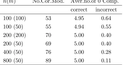
in the column “Aver.no. of 0 Comp”, where “correct” is the average number for the true nonzero components, and “incorrect” is the number of components which are erroneously set to zero. We note that for n = 100, about 50% of the estimates correctly identify the true model in the independent case; in the correlated case, this rate is about 30%. As the sample increases, the performance of model selection improves greatly. In both independent and correlated cases, the rate of identifying the correct model structure is about 70% when

n= 200 and close to 90% whenn= 800.

n(m) No.Cor.Mod. Aver.no.of 0 Comp. correct incorrect

100 (100) 53 4.95 0.64

100 (50) 55 4.94 0.55

200 (200) 70 5.00 0.40

200 (50) 69 5.00 0.40

400 (50) 76 5.00 0.28

800 (50) 89 5.00 0.11

Table 4.1: Model selection results for the independent case.

n(m) No.Cor.Mod. Aver.no.of 0 Comp. correct incorrect

100 (100) 32 4.65 0.71

100 (50) 27 4.64 0.55

200 (200) 69 5.00 0.43

200 (50) 73 4.99 0.36

400 (50) 85 5.00 0.20

800 (50) 88 5.00 0.15

Table 4.2: Model selection results for the correlated case (ρ= 0.5).

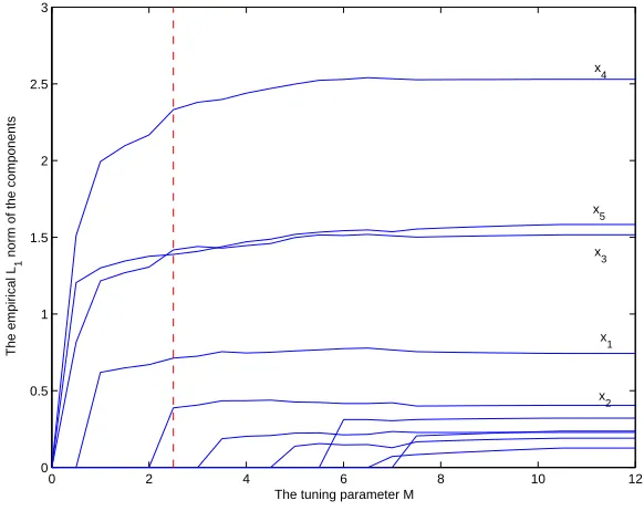
We measure the magnitude of each function component by its empiricalL1 norm defined

as 1/nPn

i=1|ηα(x (α)

i )| forα = 1, ..., d. Figure 4.1 shows how the empirical L1 norms of the estimated components change with the tuning parameter M in one simulation. The ACV

criterion chooses ˆM = 2.5, resulting a correct model of five components. To assess the goodness of function estimation, we also compute the integrated square error

ISE=EX{η(X)−ηM(X)}2,

does not degrade the performance of our method in term of estimation accuracy. Furthermore, the ISE decreases substantially while the sample size increases.

n(m) cov=0 cov=0.5

100(100) 3.91(0.11) 4.08(0.22) 100(50) 3.86(0.13) 4.12(0.20) 200(200) 1.17(0.05) 1.02(0.05) 200(50) 1.10(0.05) 0.89(0.05) 400(50) 0.36(0.02) 0.32(0.02) 800(50) 0.14(0.01) 0.16(0.01)

Table 4.3: The average ISE in 100 runs (in parenthesis are the standard errors).

0 2 4 6 8 10 12

0 0.5 1 1.5 2 2.5 3

The tuning parameter M

The empirical L

1

norm of the components

x

4

x₅

x₃

x₁

x

2

Figure 4.1: The empiricalL1 norms of the estimated components against the tuning

param-eter M. The dashed line indicates the optimal ˆM = 2.5 chosen by the ACV. Here n= 200 andm= 50.

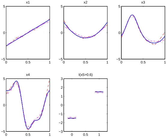
Figure 4.2 plots the true functional components and their estimates for the independent case with n = 100, m = 50. The 5th, 50th, 95th best estimates over 100 runs are ranked according to their ISE values. We can see that the proposed method provides very good estimates for those important functional components. Figure 4.3 shows the fitting results for the correlated case; here n = 800 and m = 50. It is observed that, when the sample size

0 0.5 1 −5

0 5

x1

0 0.5 1

−5 0 5

x2

0 0.5 1

−5 0 5

x3

0 0.5 1

−5 0 5

x4

0 0.5 1 −3

−2 −1 0 1 2 3

I(x5>0.6)

Figure 4.2: The estimated function components for the independent case withn= 100, m= 50. Blue solid lines are the true components; red dashed lines indicate the 5th best; magenta dashed-dotted lines indicate the 50th best; black dotted lines are the 95th best.

0 0.5 1

−5 0 5

x1

0 0.5 1

−5 0 5

x2

0 0.5 1

−5 0 5

x3

0 0.5 1

−5 0 5

x4

0 0.5 1 −3

−2 −1 0 1 2 3

I(x5>0.6)

5

Real Data Examples

5.1 Lung Cancer Data

This data was collected from the Veteran’s Administration lung cancer trial, and available in Kalbfleisch and Prentice (2002) pp.378-379. There are 137 patients in the study and 9 censored observations among those. The main interest is to study the dependence of the survival time in days on the covariates listed in the following:

treatment, 1=standard, 2=test.

celltype, 1=squamous, 2=smallcell, 3=adeno, 4=large. Karnofsky performance score (10, 20, ..., 100=good). months from diagnosis to randomization.

age in years.

prior therapy 0=no, 1=yes.

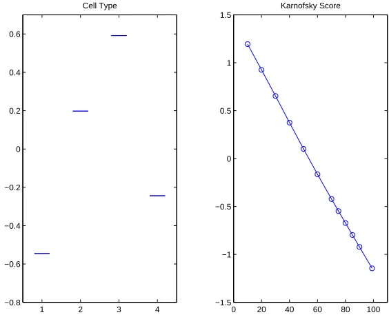
When the parametric Cox’s proportional hazard model is fitted, the stepwise selection proce-dure using the Mallow’s Cp criterion chooses two important variables: Karnofsky performance score and celltype. The linear coefficient estimates for celltype are respectively: −0.550 for squamous, 0.166 for small cell, 0.608 for adeno, and -0.224 for large cell.

1 2 3 4

−0.8 −0.6 −0.4 −0.2 0 0.2 0.4 0.6

Cell Type

0 20 40 60 80 100 −1.5

−1 −0.5 0 0.5 1 1.5

Karnofsky Score

Figure 5.1: The fitted main effects for lung cancer data.

The component estimates of our method are plotted in Figure 5.1. The coefficients for dif-ferent cell types are: −0.545 for squamous, 0.198 for small cell, 0.592 for adeno, and −0.244 for large cell. These estimates are quite close to those obtained by the linear model. Note that the component estimate of Karnofsky performance score in Figure 5.1 demonstrates a linear trend, which suggests that a linear fit may be sufficient for this data. We point out that, the LASSO studied in Tibshirani (1997) chooses only one important variable: Karnof-sky performance score, where a linear form was used for η and the celltype was treated as continuous.

5.2 PBC Data

The primary biliary cirrhosis (PBC) data was gathered from the Mayo Clinic trial in primary biliary cirrhosis of liver conducted between 1974 and 1984. This data is provided in Therneau and Grambsch (2000), and a more detailed account can be found in Dickson et al. (1989). In this study, 312 patients from a total of 424 patients who agreed to participate in the randomized trial are eligible for the analysis. For each patient, clinical, biochemical, serologic, and histologic parameters are collected. Of those, 125 patients died before the end of follow-up. We study the dependence of the survival time on the following selected covariates:

1 Continuous variables age: age in years

alb: serum albumin in gm/dl alk: alkaline phosphatase in U/liter bil: serum bilirunbin in mg/dl chol: serum cholesterol in mg/dl cop: urine copper in µg/day plat: platelets per cubic ml/1000

prot: standardized prothrombin time in seconds sgot: liver enzyme (now called AST) in U/ml trig: triglycerides in mg/dl

2 Categorical variables

asc: 0, absence of ascites; 1, presence of ascites

ede: 0 no edema; 0.5 untreated or successfully treated; 1 unsuccessfully treated edema hep: 0, absence of hepatomegaly; 1, presence of hepatomegaly

sex: 0, male; 1, female

spid: 0, absence of spiders; 1, presence spiders

We restrict our attention to the 276 observations without missing values in the covariates. As reported in Tibshirani (1997), the stepwise selection chooses eight variables: age, ede, bili, alb, cop, sgot, prot and stage. The LASSO procedure selects three more variables, sex, asc and spid. Compared to the stepwise selection, our procedure selects two more variables sex and chol. Quite interestingly, the stepwise model selects only those covariates with absolute Z-scores larger than 2.00, and our model selects only those covariates with absolute Z-scores larger than 1.00, where Z-scores refer to as the scores obtained in the full parametric Cox proportional hazard model. The LASSO, instead, selects two covariates asc (Z-score 0.23) and spid (Z-score 0.42) with Z-scores less than 1 while leaving chol (Z-score 1.11) out of the model. The fitted effects of our model are shown in Figure 5.2. The model fit suggests a nonlinear trend in cop, which is interesting and worth further investigation.

20 40 60 80

−0.8 −0.6 −0.4 −0.2 0 0.2 0.4 0.6 age

2 3 4 5

−0.8 −0.6 −0.4 −0.2 0 0.2 0.4 0.6 alb

0 10 20 30 −1 −0.5 0 0.5 1 bili

0 200 400 600 −0.3 −0.2 −0.1 0 0.1 0.2 0.3 chol

0 0.5 1

−0.4 −0.2 0 0.2 0.4 0.6 0.8 ede

8 10 12 14 16 18 −0.6 −0.4 −0.2 0 0.2 0.4 0.6 prot

0 0.5 1

−0.2 −0.1 0 0.1 0.2 sex

0 200 400

−0.5 0 0.5 sgot 2 4 −1 −0.5 0 0.5 1 stage

0 200 400 600 −0.5

0 0.5

cop

Figure 5.2: Fitted main effects for PBC data.

5.3 Mouse Leukemia Data

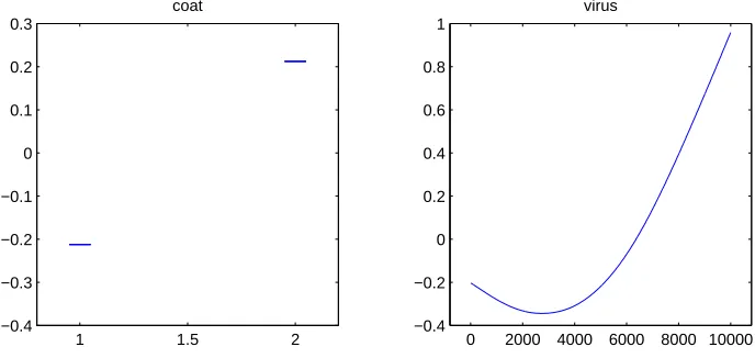
level (PFU/ml), and three categorical predictors: mhc phenotype (1 or 2), sex (1=male, 2=female) and coat color (1 or 2). The data set contains 175 mice after removing incomplete observations. We compare our analysis with the parametric model selection, which is obtained by using the backward deletion option of the function stepAIC in the R library. The linear model selection gives a final model containing antibody as the only significant factor, and the result is summarized in Table 5.1.

(a) First step, log likelihood = −264.93 Coef. Std.Err Z stat. mhc −1.00e−02 2.56e−01 −0.0391

sex 2.71e−01 2.65e−01 1.025 coat 2.36e−01 2.45e−01 0.965 antibody −1.90e−02 8.38e−03 −2.26 virus 1.24e−05 3.11e−05 0.3981

(b) Last step, log likelihood =−265.90 Coef. Std.Err Z stat. antibody −1.67e−2 6.84e−3 −2.44

Table 5.1: Results of linear variable selection for mouse leukemia data.

Our nonlinear procedure selects virus and coat as the important covariates, and the fitted main effects are plotted in Figure 5.3. It suggests a strong nonlinear trend of the log hazard in virus. Hastie and Tibshirani (1990) analyzed the same data using a backward stepwise procedure in generalized additive models, with fixed degrees of freedoms four for antibody and virus. They concluded with a final model consisting of virus level and coat color. This agrees with our result.

1 1.5 2

−0.4 −0.3 −0.2 −0.1 0 0.1 0.2 0.3

coat

0 2000 4000 6000 8000 10000

−0.4 −0.2 0 0.2 0.4 0.6 0.8 1

virus

6

Discussion

We generalized the regularization with the COSSO penalty to the nonparametric Cox’s pro-portional hazard models. An efficient criterion is proposed to select the smoothing parame-ter. The new procedure conducts model selection and function estimation simultaneously for the time-to-event data. Numerous examples suggest the great potential of this method for identifying important risk factors and estimating the components in nonparametric hazard regression.

In this work, we assumed the Cox’s proportional hazard model, which is very popular for studying survival data. However, the proportionality assumption may not hold in many situations. There are two ways to generalize the proposed method to the cases where the Cox model assumption is not proper. We can consider the following accelerated failure time models analogous to the classical linear regression approach,

log(T) =µ+η(X_{) +σW,}

whereµis a constant and W is the error distribution. Another possibility is to consider the full hazard function as h(t|x_{) = η(t,}x_{). Chapter 7 of Gu (2002) gives a discussion on this} estimate in the usual SS-ANOVA models, where the smooth estimate of the baseline hazard is incorporated into the model, and the time covariate interaction can be explored in the functional decomposition. We will explore the performances of our methods for both models in the future.

References

Aronszajn, N. (1950). Theory of reproducing kernels. Trans. Amer. Math. Soc., 68:337–404.

Breslow, N. (1974). Covariance analysis of censored survival data. Biometrics, 30:89–99.

Cox, D. R. (1972). Regression models and life-tables (with discussion). Journal of the Royal Statistical Society, Series B, Methodological, 34:187–220.

Cox, D. R. (1975). Partial likelihood. Biometrika, 62:269–276.

Dickson, E., Grambsch, P., Fleming, T., Fisher, L., and Langworthy, A. (1989). Prognosis in primary biliary cirrhosis: model for decision making. Hepatology, 10:1–7.

Fan, J. and Li, R. (2002). Variable selection for Cox’s proportional hazards model and frailty model. The Annals of Statistics, 30(1):74–99.

Gray, R. J. (1992). Flexible methods for analyzing survival data using splines, with applica-tion to breast cancer prognosis. Journal of the American Statistical Association, 87:942– 951.

Gray, R. J. (1994). Spline-based tests in survival analysis. Biometrics, 50:640–652.

Gu, C. (1996). Penalized likelihood hazard estimation: A general procedure.Statistica Sinica, 6:861–876.

Gu, C. (2002). Smoothing Spline ANOVA Models. Springer-Verlag.

Gu, C. and Wahba, G. (1991). Minimizing Gcv/gml scores with multiple smoothing pa-rameters via the Newton method. SIAM Journal on Scientific and Statistical Computing, 12:383–398.

Hastie, T. and Tibshirani, R. (1990). Generalized additive models. Chapman & Hall Ltd.

Ibrahim, J. G., Chen, M.-H., and MacEachern, S. N. (1999). Bayesian variable selection for proportional hazards models. The Canadian Journal of Statistics, 27:701–717.

Kalbfleisch, J. D. and Prentice, R. L. (2002). The statistical analysis of failure time data. John Wiley and Sons.

Kim, Y.-J. and Gu, C. (2004). Smoothing spline gaussian regression: more scalable com-putation via efficient approximation. Journal of the Royal Statistical Society Series B, 66(2):337–356.

Kooperberg, C., Stone, C. J., and Truong, Y. K. (1995). Hazard regression. Journal of the American Statistical Association, 90:78–94.

Lin, X., Wahba, G., Xiang, D., Gao, F., Klein, R., and Klein, B. (2000). Smoothing spline Anova models for large data sets with Bernoulli observations and the randomized Gacv. The Annals of Statistics, 28(6):1570–1600.

Lin, Y. and Zhang, H. (2002). Component selection and smoothing in smoothing spline analysis of variance model. Technical Report 1072, University of Wisconsin, Madison.

O’Sullivan, F. (1988). Nonparametric estimation of relative risk using splines and cross-validation. SIAM Journal on Scientific and Statistical Computing [Formerly: SIAM Jour-nal on Scientific Computing], 9:531–542.

Ruppert, D. and Carroll, R. J. (2000). Spatially-adaptive penalties for spline fitting. The Australian and New Zealand Journal of Statistics, 42(2):205–223.

Therneau, T. M. and Grambsch, P. M. (2000). Modeling survival data: extending the Cox model. Springer-Verlag Inc.

Tibshirani, R. (1996). Regression shrinkage and selection via the lasso. Journal of the Royal Statistical Society, Series B, Methodological, 58:267–288.

Tibshirani, R. (1997). The lasso method for variable selection in the Cox model. Statistics in Medicine, 16:385–395.

Wahba, G. (1990). Spline Models for Observational Data. Society for Industrial and Applied Mathematics.

Xiang, D. and Wahba, G. (1996). A generalized approximate cross validation for smoothing splines with non-Gaussian data. Statistica Sinica, 6:675–692.

Zhang, H., Wahba, G., Lin, Y., Voelker, M., Ferris, M., Klein, R., and Klein, B. (2004). Variable selection and model building via likelihood basis pursuit. Journal of the American Statistical Association, 99:659–672.