Constructing Large-Scale Genetic Maps Using an Evolutionary Strategy Algorithm
D. Mester, Y. Ronin, D. Minkov, E. Nevo and A. Korol
1Institute of Evolution, University of Haifa, Haifa 31905, Israel Manuscript received July 23, 2003
Accepted for publication August 28, 2003
ABSTRACT
This article is devoted to the problem of ordering in linkage groups with many dozens or even hundreds of markers. The ordering problem belongs to the field of discrete optimization on a set of all possible orders, amounting ton!/2 fornloci; hence it is considered an NP-hard problem. Several authors attempted to employ the methods developed in the well-known traveling salesman problem (TSP) for multilocus ordering, using the assumption that for a set of linked loci the true order will be the one that minimizes the total length of the linkage group. A novel, fast, and reliable algorithm developed for the TSP and based on evolution-strategy discrete optimization was applied in this study for multilocus ordering on the basis of pairwise recombination frequencies. The quality of derived maps under various complications (dominant vs. codominant markers, marker misclassification, negative and positive interference, and missing data) was analyzed using simulated data withⵑ50–400 markers. High performance of the employed algorithm allows systematic treatment of the problem of verification of the obtained multilocus orders on the basis of computing-intensive bootstrap and/or jackknife approaches for detecting and removing questionable marker scores, thereby stabilizing the resulting maps. Parallel calculation technology can easily be adopted for further acceleration of the proposed algorithm. Real data analysis (on maize chromosome 1 with 230 markers) is provided to illustrate the proposed methodology.
A
N important step in generating multilocus genetic of ordering markers within linkage groups was based on maps using the results of linkage analysis is the deter- multipoint maximum-likelihood analysis. Several effective mination of the true marker order. One of the possibilities algorithms have been proposed using various optimiza-in addressoptimiza-ing this problem is to recover the loptimiza-inear tion tools, including the branch and bound method marker order from the known pairwise marker distance (Lathropet al.1985), simulated annealing (Thompsonmatrixdij. A primary difficulty in ordering genetic loci 1984;WeeksandLange1987;Stam1993;Jansenet al.
using linkage analysis is the large number of possible 2001), and seriation (BuetowandChakravarti1987). orders: fornloci on a chromosome,n!/2 distinct orders OlsonandBoehnke(1990) compared eight different should be evaluated. In real problems, n might vary methods for marker ordering. In addition to multilocus from dozens to 200–500 markers and more (e.g., likelihood, they also considered more simple criteria www.maizemap.org/ibm_frameworkmaps.htm; see also for preliminary multipoint marker ordering in
large-Ott1991). Clearly, even for n ⵑ 30, it would not be scale problems based on two-point linkage data (by min-feasible to evaluate alln!/2 possible orders using two- imizing the sum of adjacent recombination rates or adja-point linkage data. This is why multilocus ordering is cent genetic distances). The simple criteria are founded considered as a nonpolynomial (NP)-hard combinato- on the biologically reasonable assumption that the true rial problem (Wilson1988;OlsonandBoehnke1990; order of a set of linked loci will be the one that
mini-Falk1992;Ellis1997). A solution to this problem can mizes the total map length of the chromosome segment. be obtained on a Pentium-IV (1500 Mhz) computer Simple methods work quickly but their accuracy may even for a modest case such asn⫽ 10 after 1 hr. depend on the number of markers, distribution of re-Several methods have been proposed for determina- combination frequencies (presence of large gaps), per-tion of marker order (Lathropet al.1985;Landerand centage of missing data, type of the employed
optimiza-Green 1987; Knapp et al. 1995; Newell et al. 1995; tion criterion, noise caused by misclassification, and
Liu1998) and implemented in software packages like genetic interference. That is why there is a tendency to LINKAGE (Lathrop et al. 1984), MapMaker (Lander combine two-point analysis with more general multipoint et al.1987), FastMap (Curtis andGurling 1993), and methods. However, even for simple methods, based on JoinMap (Stam1993). Historically, the main approach pairwise analysis, there is a pressing need for efficient algorithms enabling high-quality “preliminary” multipoint ordering. Keeping in mind the large number of markers employed in mapping projects of different organisms
1Corresponding author: Institute of Evolution, University of Haifa,
Haifa 31905, Israel. E-mail: [email protected] (humans, experimental model organisms, and
tural plants and animals), such algorithms should cope elements of ES algorithms and their correspondence with the elements and processes of an “evolving popula-with many dozens and even hundreds of markers (e.g.,
100⫼1000) per chromosome and in a reasonable exe- tion” are presented in Table 1.
The common ES algorithm steps:Evolution strategies cuting time.
We present in this article a new, highly efficient algo- define the size of a population and the rules for the selection process. Various approaches were proposed rithm of multilocus ordering based on two-locus linkage
data that employs the evolutionary optimization strategy for choosing the population size in the ES, including the (1 ⫹ 1) strategy (Rechenberg 1973) and (, ) (ES). ES is a heuristic algorithm mimicking natural
pop-ulation processes. The numerical procedures in such strategy (Schwefel 1977). With the (1⫹ 1) strategy, population size is equal to one individual used to obtain optimization are based on simulation of mutation and
reproduction, followed by selection of the fittest “geno- offspring individuals via mutation operation. If a new individual is better than the “parent,” it replaces the types,” representing the obtained values of the
optimiza-tion criterion. Together with genetic algorithm (Hol- parent. The (,) strategy works with a population of size. The selection operator choosesbest individuals
land1975) and evolutionary programming (Fogel1992),
evolution strategies form the class of evolutionary algo- to establish the new generation. Both versions, (1⫹1) and (,), employ the following steps:
rithms (Nissen 1994). The evolutionary strategies were proposed in the 1970s (Rechenberg 1973; Schwefel
1. Create individuals (xk) of initial populationP0. 1977, 1987) to solve optimization problems with
real-2. Compute the fitnessf(xk), k⫽1, . . . ,. value variables. A recent survey of search strategies for
3. If the optimization process is terminated, then stop. combinatorial problems was provided byMuhlenbein
4. Select the ⱕ best individuals. et al.(1998). ES for optimization problems is presented
5. Create/offspringxk⫹1of each of the individu-as a random search by individu-asexual reproduction, which uses
als by small variation. mutation-derived variation and selection. The mutation
6. Return to step 2. change of the current vector of parameters can be
intro-duced by adding a vector of normally distributed vari- Peculiarities of the combinatorial version of ES:
Clearly the multilocus ordering problem cannot be di-ables with zero means. The level of changes can be
adapted by variances of these disturbances. rectly represented in terms of ES with real-value formu-lation. Combinatorial versions of ES differ from the In contrast to ES, genetic algorithms, introduced by
Holland(1975), simulate sexual reproduction that is real-value formulation by specific representation of the
solution vector x and mutation mechanisms (
Hom-characterized by recombination of two parental strings
to build the offspring generation. Clearly, the contribu- bergerand Gehring1999). In combinatorial formula-tion, the solution (an “individual”) can be represented as tions ofmutationandrecombinationas sources of variation
in the search strategy are different: mutation is based a vectorx⫽(x1,x2, . . .xn) that consists ofnranked discrete
coordinates (chromosomes) or as a directed graphG(A, on chance only, and the success of a single mutation
is largely unpredictable. Crossover can be viewed as a B) with a set of nodes A ⫽ {a1, a2, . . . an} and set of
arcs B ⫽ A ⫻ A, where node aj,j ⬎ 0, represents the
history-preserving operation, which at the same time
introduces a new structure to be tested in competition. chromosome. The fitness function assigns to each of the n(n⫺1)/2 arcs (ai,aj) [or pair of coordinates (xi,xj)] a
HombergerandGehring(1999),Mester(1999, 2000),
andD. Mester (unpublished results) adopted the ES nonnegativedijcost of moving from elementito element
j. The problem is symmetric if and only ifdij ⫽ dji for
algorithm to solve the vehicle routing problem with
time-window restrictions, which is similar, to some ex- all arcs. For optimization of a combinatorial problem, one needs to define such an order of the vector coordi-tent, to multipoint analysis of markers belonging to
several chromosomes (linkage groups). In this article, nates (or nodes) that will provide minimum total cost. The mutation operator (referred to hereafter as muta-we applied the ES algorithm for multipoint marker
or-dering using the similarity between this problem and tor) changes the vector xk, thereby producing a new solution vectorxk⫹1. For this goal, one can use the move-the well-known traveling salesman problem (TSP;Press
et al.1986;WeeksandLange1987;Falk1992;Schiex generationand thesolution-generationmechanisms (Osman
1995;HombergerandGehring1999) or theremove-insert
andGaspin1997).
mechanism (Mester1999). Our version of the combi-natorial ES algorithm employs multiparametric mutator
EVOLUTION STRATEGIES AND THE HEURISTICS (MPM), which changes the solution vector via removing
IN THE DEVELOPED ALGORITHM
and inserting  coordinates of xk (Mester 1999; D.
Mester, unpublished results). The common heuristic
The employed procedure as a simulated analog of
evolutionary processes: Usually, the optimization pro- removedefines a random proportion ⫽(0.1⫹0.5r)n of rejected coordinates in the solution vector, wheren cess of an objective functionf(x) withnreal-value
vari-ables x ⫽ (x1, x2, . . . , xn) can be represented as an is the number of coordinates in the solution andris a
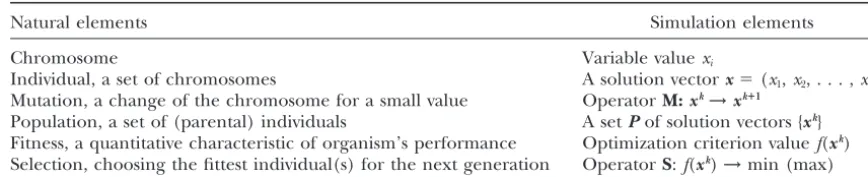
TABLE 1
Main components of ES algorithm as a simulation analogue of evolutionary models
Natural elements Simulation elements
Chromosome Variable valuexi
Individual, a set of chromosomes A solution vectorx⫽(x1,x2, . . . ,xn)
Mutation, a change of the chromosome for a small value OperatorM:xk→xkⴙ1
Population, a set of (parental) individuals A setPof solution vectors {xk}
Fitness, a quantitative characteristic of organism’s performance Optimization criterion valuef(xk) Selection, choosing the fittest individual(s) for the next generation OperatorS:f(xk)→min (max)
1. The heuristic also defines a set of removing rulesR rithm provides quality solutions and is faster than other adaptive algorithms (GLS, SA, and TS).
(to take out specific parts ofxkor the full vector). At
Multipoint marker ordering as a TSP problem:The this mutation stage, the solution vectorxkis divided into
proposed algorithm of multipoint ordering employs two subvectors: xk
remainder and xkreject. Another common
two-point linkage data (see alsoPresset al.1986;Weeks
heuristic,insert, defines a set of rulesIto insert,
conse-andLange1987;Falk1992;SchiexandGaspin1997).
quently one by one, allxi僆xkrejectintoxkremainder. This is
Although this approach is usually considered as “prelim-theconstruction phaseof the mutator, which builds some
inary ordering,” the good quality of the maps produced new solution vectorsxk⫹1using the variation of the
prob-by our version of the ES algorithm (see below) allows lem-specified criterion (Mole and Jameson 1976; Or
us to consider it not only as a complement to the more 1976;Osman1993;Mester1999).
sophisticated multilocus maximum-likelihood (ML) or-At themutation stage, mutatorM(R, I,,xk) produces
dering, but also, to some extent, as a competitor to ML an offspringxkⴙ1from the parentxk. If the first offspring
algorithms (especially for a large number of marker loci appears to surpass the parent, the mutator with the
and various complications like missing data, misclassifi-same parameters is applied again to the new parent,
cation, etc.). We considern markers enumerated arbi-and so on. If the offspring does not surpass the parent,
trarily by n coordinates xi 僆 x and, for each n ⫺ 1
then to generate the new offspring, the algorithm uses
marker pairs (xi,xj), a “distance”ij. Asij, either pairwise
the mutator with other parameters. After mutation, the
recombination fractionsrijor map distances dij(e.g., in
vectorxk⫹1“is improved” by standard combinatorial
pro-Haldane or Kosambi metrics) are employed. cedures of orderO(n2): (1) 2-Opt (LinandKernighan
Different criteria can be used to discriminate between 1973), (2) Or-Opt (Or 1976), and (3) 1-interchange
competitive orders, for example, total distance
mea-(Osman1993).
sured as a sum of distances between consecutive adja-This two-phase approach (mutation-improving)
re-cent markers or the total number of recombination flects the principles of solution diversification and
up-events. These criteria are founded on a biologically rea-grading (Rochat and Taillard 1995). We combine
sonable assumption that the true order of a set of linked the last three improving procedures into one composite
loci will be the one that minimizes the total length of procedure (Composite). At the initial solution phase,
the chromosomal map (Presset al. 1986; Weeks and Composite is applied five times. We refer to such an
Lange1987;Falk1992;SchiexandGaspin1997). In
algorithm (multiple application of the Composite
pro-our model, the minimum of sum of distances between cedure starting from random initial points) as the
Multi-adjacent markers was applied as optimization criterion Startprocedure. In Table 2 we compare the solutions
(OC), of standard TSP obtained by four different powerful
heuristics: guided local search (GLS), simulated
anneal-OC ⫽
兺
n
ij
ij␦ij, (1)
ing (SA), tabu search (TS; for the comparison of these three algorithms, seeVoudorisandTsang1999), and
the ES-MPM algorithm proposed by Mester (1999, where␦ij⫽0 or␦ij⫽1 represents in the criterion only
2000, and unpublished results). In addition, we present u ⱕ n ⫺ 1 distances out of all n(n ⫺ 1)/2 pairwise for comparison also three simple heuristics: 3-OPT of distances;ij␦ij ⬎0,i⫽1,n⫺1;j⫽2,n.
Lin and Kernighan (1973), the Composite, and the The program for simulations was written in Visual
Multi-Start (Table 2). ES-MPM is a two-phase algorithm Basic 6.0. Monte Carlo testing experiments were con-that first produces an initial solution using the simple ducted on a double-processor Pentium 3 (800 Mhz). Multi-Start procedure and then moves to a more power- To compare different situations, the following coeffi-ful, albeit less fast, ES-search (ES-phase). The presented cient ofrestoration quality[proximity between the “true”
algo-TABLE 2
Comparison of different heuristics and the ES-MPM algorithm on standard (51–318 points) TSP
Inaccuracya(I, %) and executing time (T, sec)
Best of the TSP solutions
GLS Problem published
N name solutions ES-MPM SA TS 3-Opt Multi-Start Composite
1 Ei1-51 426 I 0 0 0.73 0 5.9 2.0 3.4
T 1.3 0.1 6.3 1.1 0.2 0.04 0.01
2 Eil-101 629 I 0 0 1.76 0 4.8 5.0 5.0
T 5.0 1.3 33.3 61.4 0.2 0.2 0.04
3 Eil-76 538 I 0 0 1.21 0 3.5 4.3 4.7
T 2.3 1.1 18 5.2 0.1 0.08 0.01
4 KroA-100 21,282 I 0 0 0.42 0 0 0.2 6.5
T 0.7 0.6 37.4 21.4 0.12 0.3 0.06
5 KroA-150 26,524 I 0 0 1.86 0.03 8.4 5.2 4.8
T 24 103.3 413 0.8 0.35 0.27
6 KroA-200 29,368 I 0 0 1.04 0.72 4.6 4.8 6.6
T 187 34 229.4 776 4.3 0.3 0.9
7 KroC-100 20,749 I 0 0 0.8 0.25 4.5 4.3 7.7
T 1.8 1.5 36.6 4.8 0.3 0.2 0.07
8 Lin-318 42,029 I 0 0 1.34 1.31 4.0 4.2 5.6
T 335 245 829 2672 13.8 7.6 0.8
aInaccuracy is employed as a score of the quality of the solution; it is presented as a deviation (%) of the
obtained result (by the inspected method) from the best-known solution.
2. defined proportion of dominant vs. codominant Kr⫽ (n⫺ 1)/
兺
n⫺1
i⫽1
冨
xi⫺xi⫹1冨
, (2)markers;
3. chosen proportion of missing data; wherexiis the digit code of theith marker in the currently
4. chosen proportion of markers with erroneous classi-ordered marker sequence. Figure 1 illustrates a typical
fication and level of errors; and
dependence of Kr on executing time using different 5. chosen mode of recombination interference for adja-heuristics.
cent markers, Haldane, Kosambi, or arbitrary inter-ference. In the last case, we define a few ranges of coincidence values and the probabilities to sample
SIMULATED DATA SETS
the coincidence values from these ranges (with even The data for analysis were produced using a
pseudo-distribution of the coincidence values from the cho-random generator. The simulation algorithm
repeat-sen range). edly generated a single-chromosome mapping
popula-The following are the numerical values (ranges) of tion, F2, for a chosen number of markers with:
the main parameters in the majority of experiments: 1. Variation of recombination rates between adjacent
markers along the chromosome; 1. The number of markers per chromosome:m⫽ 80.
Figure 1.—Typical dependence of order quality (Kr) on executing time
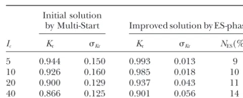
TABLE 3 2. Probability distributions for distances between
adja-cent markers: Effect of negative interference on the quality of P(3 ⬍ d (cM) ⬍ 5)⫽ 0.8, P(5 ⬍ d (cM) ⬍ 10) ⫽ multilocus ordering
0.15,P(10⬍d(cM)⬍20)⫽0.05, with even
distribu-tion within each of the three ranges. Initial solution
by Multi-Start Improved solution by ES-phase
3. Proportions of codominant and dominant markers (in coupling phase, unless noted otherwise): 0.5 and I
c Kr Kr Kr Kr NES(%)
0.5, respectively.
5 0.944 0.150 0.993 0.013 9
4. Three levels for missing data: 0, 10, and 20%.
10 0.926 0.160 0.985 0.018 10
5. Two levels for the proportion of loci with
classifica-20 0.900 0.129 0.937 0.043 11
tion errors, 0 and 40%, and in the last case, two levels 40 0.866 0.125 0.901 0.056 14 of misclassification, 10 and 20%.
Icis the maximum value of the coincidence coefficient for
6. In the case of arbitrary interference, the distributions
cases of negative interference; as noted in the description of
of coincidence coefficients:P(0⬍c⬍1)⫽0.6
(posi-the simulation procedure,P(2⬍ c ⬍ Ic) ⫽ 0.2
(moderate-tive interference), P(1 ⬍ c ⬍ 2) ⫽ 0.2 (slight- to-strong negative interference; in more detail, the analyzed to-moderate negative interference), andP(2 ⬍ c⬍ situations are described insimulated data sets). Note the Ic) ⫽ 0.2 (moderate-to-strong negative interference), increased stability of ordering owing to application of the
ES-phase of the ES-MPM algorithm (displayed in a substantial
whereIc⫽5, 10, 20, and 40.
reduction in the standard deviation,Kr, of the coefficient of
restoration quality,Kr. Here and in the following tables,NES Therefore, the efficiency of the preliminary multilocus
is the proportion of cases (Monte Carlo runs) where
applica-ordering was considered upon complications caused by
tion of the ES-phase after the Multi-Start procedure improved
negative interference, erroneous marker scoring, and
the solution.
incomplete mapping information due to dominant markers and missing data, known to affect the quality of
multipoint ordering. Motivation to consider such compli- repulsion phase, the lower the quality of multilocus cations derives from the simple fact that in real mapping ordering (Mester et al. 2003). The employing of the work no one can guarantee that the data are free of ES-phase of the ES-MPM algorithm (see above, Peculiari-such complications. Moreover, in numerous previous
ties of the combinatorial version of ES) after getting some attempts at building efficient multilocus ordering tools, initial solution through Multi-Start positively affected some of these problems were usually ignored. the quality of the final solution. It is noteworthy that
the application of ES-phase also stabilizes the ordering results (as displayed by the reduction ofKr, the standard
RESULTS
deviation ofKrbetween the Monte Carlo experiments). High precision of ordering in the coupling-phase data The considered types of disturbances (see the end of
simulated data sets) proved to affect the quality of and low precision in the repulsion-phase data justify
splitting the data into two sets, each with coupling-phase restoration of the true order of markers. These
distur-bances mainly caused local distortion of the order,e.g., markers only and generating two complementary maps for each linkage group (Knapp et al.1995; Penget al. interchanging of two to three neighboring markers
(re-ferred to as “local disturbances”). There could be several 2000;Mesteret al.2003). Clearly, the next step should be integration of the two maps. The last step may en-inverted islands per linkage group. As expected, the
number of these islands increases with the percentage counter difficulties caused by local and global map dis-turbances affecting codominant markers common for of missing data, classification errors, and the level of
negative interference. Less frequent were violations both maps, if the density of such codominant markers is relatively low (e.g., in cases when codominant markers caused by excision of a large segment and its
transposi-tion to another place with or without inversion within serve as anchors). In fact, the availability of shared co-dominant markers enables mutual control during multi-the segment (“global disturbances”). Clearly, such
viola-tions result in an appreciable reduction of the coeffi- locus ordering, which, together with computing-inten-sive jackknife and bootstrap techniques (Efron1979), cient of restoration quality (Equation 2).
Dominance:When all dominant markers were in cou- significantly improves the quality of the resulting map
(Mesteret al. 2003).
pling phase, the proportion of dominant and
codomi-nant markers had no effect on the quality of marker Negative interference:As expected, negative interfer-ence complicates the ordering problem that is mani-ordering. For three proportions of dominant markers
(50, 66, and 100%) with Kosambi, Haldane, and a slight fested in reduction ofKr(Table 3). However, the decline inKrwith an increase in the maximum valueIcof
coeffi-negative interference, nearly full recovery of marker
order was reached (Kr ⬇ 0.997 ⫼ 0.999). A different cient of coincidence c is unexpectedly slow, pointing to robustness of the employed ordering procedure. A result was obtained with dominant markers in repulsion
Figure2.—Local disturbances of the order due to negative interference.
deviations from the true order in such cases are due 20%) show the same tendencies as those found for com-mainly to interchanges of adjacent markers. The rela- plicating factors considered above. Thus, participation tively low effect of negative interference can be ex- of the ES-phase in the optimization procedure increased plained by a stabilizing role of the neighboring intervals. the precision of ordering (reducing the deviation ofKr This can be illustrated by the following example (Figure from unity) and stabilized the ordering among Monte 2), in which recombination rate between the flanking Carlo runs (as displayed in reduction ofKr).
markersM1andM3is smaller than that for the subinter- Comparison with multilocus algorithms:The forego-valM2–M3(see Figure 2a). ing results illustrate the advantages of the ordering pro-Without taking into account the information from cedure on the basis of minimization of the total length neighboring intervals, the criterion “minimum of total of the map (sum of recombination rates or distances distance between markers” will give the local orderM2– between consecutive pairs of markers). Combined with M1–M3(Figure 2b) that differs from the true one. The our novel, highly efficient method of discrete optimiza-stabilizing effect of the neighborM0allows us to obtain tion, a unique performance and rather high robustness the true order. Indeed, the optimization criterion value with respect to various disturbances (like classification for the true order (Figure 2c) is OC⫽0.048⫹0.024⫹ errors, negative interference, and missing data) are pro-0.059⫽0.131, whereas the order corresponding to the vided. It is noteworthy that ordering 100, 200, 400, and foregoing inversion between M1 and M2 (Figure 2d) 800 markers takes ⵑ1.3 sec, 14 sec, 2 min, and 9 min caused by negative interference results in OC⫽0.072⫹ on a Pentium-4 2.0-GHz computer in the most compli-0.024⫹0.052⫽0.148. Therefore, despite high negative cated of the aforementioned situations. Note that even interference on interval M1–M2–M3 (c ⫽ 15.8), which better performance was found in the first trials of our violates the rule that “the entire entity is supposed to new optimizer based on guided evolution strategies be larger than its parts,” the algorithm recovers the true (GES): on the same computer, map ordering for the order. foregoing variants proved fivefold (!) faster (Mester
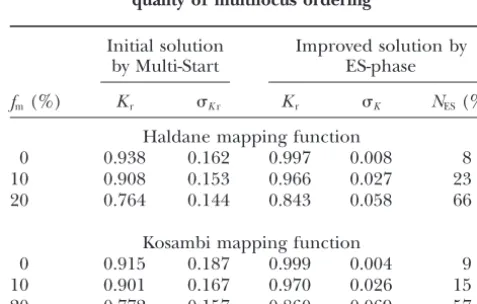
Misclassification:Errors in marker scoring inflate re- andBraysy2003). It would be of interest to compare combination distances and can also violate the
princi-ple, the entire entity is supposed to be larger than its
parts by imitating “negative interference.” This is why TABLE 4 some mapping packages allow for error filtration by
Effect of marker misclassification (fm) on the
selecting out double recombinants. Our simulations
quality of multilocus ordering showed that in the majority of such local violations the
true order could be recovered due to the stabilizing Initial solution Improved solution by effect of the neighboring markers (Table 4). by Multi-Start ES-phase
In a typical example (Table 5) with a maximum level
fm(%) Kr Kr Kr K NES(%)
of noise (20% of marker scoring errors were simulated
for 40% of marker loci), there were 14 pairs of adjacent Haldane mapping function
0 0.938 0.162 0.997 0.008 8
intervals (out of 49 possible pairs) in which eitherri,i⫹1
10 0.908 0.153 0.966 0.027 23
or ri⫹1,i⫹2 was larger than ri,i⫹2, but in only 4 of these
20 0.764 0.144 0.843 0.058 66
pairs the true order could not be recovered. We con-clude from the obtained results that despite the biases
Kosambi mapping function
in pairwise estimates of recombination rates and infla- 0 0.915 0.187 0.999 0.004 9 tion of the map length, the employed criteria of order- 10 0.901 0.167 0.970 0.026 15 ing are fairly robust to errors in marker scoring, unless 20 0.772 0.157 0.860 0.069 57
the errors occur on a catastrophic level (say, at half of
Note that the proportion of cases in which application of
the loci and with a rateⰇ20%). the ES-phase after the Multi-Start procedure improved the
Missing data: The results presented in Table 6 for solutions (NES) increased severalfold for the nonzero level of
misclassification.
TABLE 5
Effect of violations of the principle “entire is larger than its parts” caused by typing errors (20% at 40% of loci) and “self-correction” of the order owing to the stabilizing role of adjacent markers
True Resulting
order c or d r12 r23 r13 order Sign
3–4–5 c-c-c 0.125 0.197 0.123 3–4–5 ⫹
5–6–7 c-c-c 0.163 0.114 0.086 5–7–6 ⫺
12–13–15 c-c-d 0.127 0.291 0.247 12–13–15 ⫹
13–15–16 c-d-c 0.291 0.227 0.254 13–15–16 ⫹
17–18–19 c-c-c 0.174 0.148 0.092 17–18–19 ⫹
23–24–25 c-d-c 0.196 0.190 0.131 23–24–25 ⫹
25–26–28 c-c-c 0.145 0.157 0.078 25–26–28 ⫹
32–33–34 c-d-c 0.249 0.216 0.216 32–34–33 ⫺
35–36–37 c-c-d 0.270 0.196 0.166 35–37–36 ⫺
39–40–41 d-c-d 0.184 0.274 0.258 39–40–41 ⫹
40–41–42 c-d-c 0.274 0.240 0.265 40–41–42 ⫹
42–43–45 c-d-c 0.178 0.300 0.210 42–43–45 ⫹
43–45–46 d-c-d 0.300 0.119 0.231 43–45–46 ⫹
50–51–53 c-c-c 0.152 0.259 0.188 51–50–53 ⫺
c and d denote codominant and dominant markers, respectively;r12, r23, andr13are recombination rates
between markers within a triad 1, 2, and 3; recovering of the true order despite violation is denoted by “⫹,” whereas “⫺” denotes distorted order.
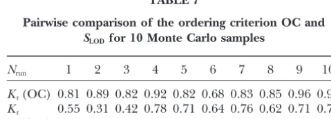
our algorithm with other procedures, like those ofOtt To compare the efficiency of the OC criterion (Equa-tion 1) with the multilocus-likelihood method, Map-(1991) and Lander and Green (1987). Ott (1991)
proposed a criterion on the basis of sliding summation Maker 3.0 software was employed in a simulated data set of 200 markers with high negative interference in of three-locus LODs along the chromosome. This
crite-rion was compared with the foregoing OC critecrite-rion (see several regions. First, we revealed on the simulated map all islands where for three consecutive markersi,i⫹1, Equation 1), using our optimization tools, on the basis
andi⫹2, eitherri,i⫹1orri⫹1,i⫹2was larger thanri,i⫹2. For
of 10 Monte Carlo samples. The simulated F2data were
each such island, three “windows” involving 5, 7, and 9 for a 100-marker map (total length 500–600 cM),
popu-markers, respectively, were analyzed using MapMaker. lation size n ⫽ 200 with a very high noise caused by
Simultaneously, the entire set of 200 markers was or-misclassification (40% of markers were simulated with
dered with our program. Despite the fact that a local 20% of typing errors!). The pairwise comparison shows
order that one could derive by comparing multilocus (Table 7) that OC does invariably better than SLOD
likelihoods for all possible candidate orders of such (higher values of the coefficient of restorationKrwere
local neighborhoods (of 5, 7, or 9 markers) cannot be obtained for OC).
considered as a final solution, it makes sense to compare the local properties of the MapMaker solutions and TABLE 6
those of the OC-based procedure (with OC defined by Effect of the missing data proportion (m) on the efficiency Equation 1). This is especially important for situations of multilocus ordering in which the natural conditionri,i⫹1andri⫹1,i⫹2⬍ri,i⫹2is
Initial solution Improved solution
by Multi-Start by ES-phase
TABLE 7
m(%) Kr Kr Kr Kr NES(%)
Pairwise comparison of the ordering criterion OC and
Haldane mapping function S
LODfor 10 Monte Carlo samples
0 0.938 0.162 0.997 0.008 8
10 0.953 0.143 0.992 0.013 16 N
run 1 2 3 4 5 6 7 8 9 10
20 0.917 0.158 0.974 0.023 17
Kr(OC) 0.81 0.89 0.82 0.92 0.82 0.68 0.83 0.85 0.96 0.95
Kosambi mapping function Kr 0.55 0.31 0.42 0.78 0.71 0.64 0.76 0.62 0.71 0.75
0 0.915 0.187 0.999 0.004 9 (SLOD)
10 0.927 0.172 0.996 0.009 14
Kr is the coefficient of restoration, whereas OC and SLOD
20 0.926 0.154 0.981 0.020 14
denote our criterion (Equation 1) and the criterion based on sliding summation of three-locus LODs.
violated, causing the highest instability of the result un-der sampling variation,e.g., by using jackknife or boot-strap procedures. It should be noted, however, that ap-plication of these last techniques seems impossible with MapMaker forⵑ100 and more markers because of CPU limitations. The following are the details of this compari-son. The simulated data of 200 markers included (a) for 95% of intervalsL⫽0.75 cM, for 2.5%L⫽30 cM, and for the remainder 2.5%L⫽60 cM; (b) 80% of the markers dominant in coupling phase, and 20% codomi-nant; (c) population sizeN⫽400; and (d) interference, with probabilityP ⫽ 0.6,c 僆(0, 1), with P⫽ 0.2,c 僆 (1, 2), withP⫽0.2, c僆(2, 20).
This example included 10 3-marker islands with viola-tion of the condiviola-tion {ri,i⫹1andri⫹1,i⫹2⬍ri,i⫹2}. In addition to negative interference or classification errors, such a violation may derive from sampling fluctuations, espe-cially when two adjacent intervals are of very different lengths. At 8 out of 10 such islands, our algorithm recov-ered the true order (the entire solution for 200 markers took⬍1 sec). MapMaker recovered the true order in 5 out of 10 islands on the basis of the 5-marker window; the remaining 5 islands were treated using the 7-marker window and recovered the true order in an additional 3 islands, and the last 2 were treated using the 9-marker window with a 50% success. The last two tasks took 6 hr.
Possibilities to validate the solution:Clearly, the fore-going comparisons using simulated data are only to illustrate the quality of the solution provided by the simple OC-based procedure. In dealing with real data,
Figure3.—Scheme of the algorithm for map verification.
one needs some tools to validate the obtained order, and it is hard to choose the solution from several (sometimes dozens) candidate solutions (like those provided by
MapMaker). To cope with this problem, some authors the putative causal factor of instability: (a) double re-proposed computing-intensive procedures based on var- combinants in adjacent intervals (resulting from nega-ious combinations of jackknifing and bootstrapping tive interference or misclassification) and (b) sampling
(Efron1979; Mottet al.1993;Wanget al. 1994;Liu variation of recombination in large intervals. The first
TABLE 8
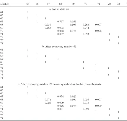
A fragment of the matrix of neighborhood frequencies based on the jackknife procedure
Marker 65 66 67 68 69 70 71 72 73 74
a. Initial data set
64 1
65 1
66 1 1
67 1 0.737 0.263
68 0.737 0.993 0.263 0.007
69 0.263 0.993 0.744
70 0.263 0.774 0.993
71 0.007 0.993 1
72 1 1
73 1 1
74 1
b. After removing marker 69
64 1
65 1
66 1 1
67 1 1
68 1 1
70 1
71 1 1
72 1 1
73 1 1
74 1
c. After removing marker 69; scores qualified as double recombinants
64 1
65 1
66 1 1
67 1 0.974 0.026
68 0.974 0.999 0.026 0.001
69 0.026 0.999 0.975
70 0.026 0.975 0.999
71 0.001 0.999 1
72 1 1
73 1 1
74 1
Multilocus ordering was conducted using the sum of recombination rates along consecutive pairs of adjacent markers.
easily seen from this fragment that two local orders are OC(s1), but it is clear that for another sample OC(s2)
may be selected as well, due to sampling variation of possible for this part of the map,s1⫽(67, 68, 69, 70) and
s2 ⫽ (67, 68, 69, 70), with probabilities P(OC(s1) ⬎ recombination rates. This is why it is important not only
to detect such questionable neighborhoods, but also to OC(s2))⫽0.737 andP(OC(s1)⬍OC(s2))⫽0.263. The
recombination rates for the two orders calculated on evaluate the probabilities of the local competitive or-ders. The same is true for any other ordering criterion, the initial data set are shown in Figure 4. Thus, the OC
values are OC(s1)⫽0.099⫹0.082⫹0.069⫽0.250 and e.g., maximum likelihood, because P(L(s1)⬎ L(s2)) is
alsoa prioriunknown. For our numerical example, the OC(s2)⫽0.143⫹0.082⫹0.029⫽0.254. Therefore, on
the basis of OC values, one will choose the true order probabilities of the compared alternative orders do not
differ significantly, so that further steps are needed to “natural” marker numbers as they are represented in the Excel data file (see alsoLee et al.2002) were used obtain a solution with higher confidence.
The simplest way to improve the quality of the solu- as a reference ordering. To address the foregoing ques-tions (a–e), we employed our ordering algorithms for tion is to remove the questionable marker (Mottet al.
1993; Liu 1998). In our example, the source of the map construction and jackknife resampling procedure to test the reliability of the resulting orders (using 100 difficulties in the island 67–70 was marker 69 that
in-flated fivefold the size of the spanning interval 68–70. jackknife runs with sampled proportion of 90% of geno-types at each run). Following are the obtained results. After removing marker 69, the jackknife procedure was
applied 1000 times again with results shown in Table First, marker 24 showed no close linkage with any of the remaining 230 markers; hence it was excluded from 8b. Thus, by deleting the problematic marker, one can
obtain an unequivocal local ordering. the map. The remaining marker groups were classified A more complex approach is based on temporal ex- with respect to the jackknife test of neighborhood sta-clusion of marker scores considered as double recombi- bility:
nants (without affecting other markers of the same
indi-1. Regions with stable (P⫽1) neighborhoods that fully viduals; see Figure 3). This increases the probability of
coincide with the published IBM map were: 1–14, recovering the true order by excluding (albeit
artifi-37–48 (without marker 39 that was linked closer to cially) the local violations of the condition ri,i⫹1 and
other markers of chromosome 1; see below), 52–60, ri⫹1,i⫹2 ⬍ri,i⫹2. After such editing of the data, we again
81–84, 89–91, 112–115, 120–125, 128–133, 140–153, applied the jackknife procedure. In the above example,
205–208, and 218–221. after 1000 runs we obtained the result shown in Table
2. Segments with neighborhood probability⬎P⫽0.90 8c. Thus, as expected, removing double recombinants
that coincide with the published map were: 18–25 resulted in an increased stability of the derived ordering:
(but without marker 24), 28–33, 63–75, 160–165, the weakest connection between the neighbors in the
168–174, and 221–231. locality 67–68–69–70 increased fromP⫽0.737 up toP⫽
3. Segments with neighborhood probability⬎P⫽ 0.9 0.974. Note that after removing double recombinants,
that did not coincide with the published map; the r68–69andr69–70decreased from 0.082 and 0.069 to 0.025
revised orders were: (1) 174–176–175–177; (2) 179– and 0.011, respectively, and r68–70 ⫽ 0.029. Therefore,
181–180, 184–185–186–188; (3) 204–202–201–205; the conditionri,i⫹1andri⫹1,i⫹2⬍ri,i⫹2is not violated
any-and (4) 214–216–215–217. more. The same procedure could be applied to test the
4. Islands with simple unresolved alternatives; for reso-second local order, namely 67–69–68–70.
lution (i.e., to reach the foregoing conditions b or
An example of application to real data:We employed
c) it is necessary to exclude 1–2 markers: the proposed approach to recently published mapping
i. 15–16–17–18 withP(15–16)⬇ 0.62vs. 15–17– data on the maizeIntermated B73⫻Mo17 (IBM)
popula-16–18 withP(15–17)⬇0.38: after marker 17 is tion(Leeet al.2002). For demonstration, the first
chro-excluded, we obtainP(15–16)⫽P(16–18)⫽1. mosome (with 231 markers) was chosen from the Map
ii. 25–27–26–39–28 with P(25–27)⬇ 0.72 vs. 25– database (www.maizemap.org/ibm_frameworkmaps.htm,
26–27–39–28 with P(25–26) ⬇ 0.28: after framework_302.xls file). In our treatment of this data
marker 27 is excluded, we obtain P(25–26)⫽ set, several questions that could be addressed during
p(26–39)⫽p(39–28)⫽1. Resolving this situa-the map construction and its validation based on
jack-tion has also improved the stability of the forego-knife were of interest: (a) to reveal the map segments
ing group 28⫼33 that can be moved now from with stable neighborhoods (P⫽1 for each pair of
adja-the set of groups withP⫽0.9 to the set of fully cent markers) that fully coincide with the published
stable ones withP⫽ 1. map (Leeet al.2002); (b) to reveal the map segments
iii. Stabilization of group 28⫼33, in its turn, caused with neighborhood probability higher than some
an improvement for group 33⫼36. Instead of threshold (e.g.,P⫽0.90 or 0.95) that coincide with the
the initial dichotomy, 33–34–35–36 withP(33– published map; (c) to reveal the map segments with
34)⬇0.78vs. 33–35–34–36 withp(33–35)⬇0.22, neighborhood probability higher than some threshold
we obtainedP(33–34)⫽0.96,P(34–35)⫽1, and (P⫽ 0.90 or 0.95) that do not coincide with the
pub-P(35–36)⫽ 0.96. lished map; (d) to demonstrate alternative
(competi-iv. 48–49–51–50–52 withP(48–49)⬇ 0.84 vs. 48– tive) orders of the same region with unreliable
neigh-50–51–49–52 withP(48–50)⬇0.16. By exclud-borhoods (i.e., with neighborhood probability lower
ing marker 51, we can get P(48–49) ⫽ 0.93, than the threshold) that could be resolved by excluding
P(49–50)⫽1, andP(50–52)⫽ 0.93. 1–2 markers to fit the conditions b or c; and (e)
reveal-v. 60–62–61–63 with P(60–62) ⬇ 0.62 vs. 60–61– ing the segments of the map for which an exclusion of
62–63 withP(60–61)⬇0.38. By excluding marker a larger group of markers (e.g.,ⱖ2) is needed to fit the
61, we obtainP(60–62)⫽P(62–63)⫽1. conditions b, c, or d for the remaining subgroups.
75–79–80–76–77–78–81 with P(75–79) ⬇ 0.4. 92–93, 96–97, 97–98, 98–100, 100–102, 102–103, 103–106, 106–105, 105–107, 107–108, 108–110, After excluding markers 76 and 77, we obtain
P(75–78)⫽0.95,P(78–79)⫽0.99,P(79–80)⫽ and 110–111, andP⫽ 0.99 for 93–96.
ii. In the second group, P(187–188) ⫽ 0.47, 1, and P(80–81)⫽0.95.
vii. 84–85–86–88–87–89 withP(84–85)⬇0.5vs. 84– P(188–189) ⫽0.61,P(189–190)⫽ 0.9,P(190– 191)⫽0.99,P(191–192)⫽0.41,P(192–193)⫽ 86–85–88–87–89 withP(84–86)⬇ 0.5.
Exclud-ing markers 86 and 87 results inP(84–85)⫽ 1,P(193–194)⫽0.66,P(194–195)⫽0.5,P(195– 196)⫽1,P(196–197)⫽0.75,P(197–198)⫽0.5, P(85–88)⫽ P(88–89)⫽1.
viii. 115–116–117–118–119 withP(115–116)⬇0.55 P(198–199) ⫽ 0.61, P(199–200) ⫽ 0.83. After excluding markers 187 and 198 we obtained vs. 115–117–118–116–119 with P(115–117) ⬇
0.45. After 116 is excluded, P(115–117) ⫽ P(188–189) ⫽ 1, P(189–190) ⫽ 0.97, P(190– 191) ⫽ 1, P(191–192) ⫽ 0.96, P(192–193) ⫽ P(117–118)⫽P(118–119)⫽ 1.
ix. 125–126–127–128 with P(125–126) ⬇ 0.56 vs. 0.98, P(193–194) ⫽ 0.97, P(194–195) ⫽ 0.96, andP⫽1 for pairs 195–196, 196–197, 197–199, 125–127–126–128 withP(125–127)⬇0.44;
ex-clusion of marker 126 gives P(125–127) ⫽ and 199–200. P(127–128)⫽ 1.
The results of these manipulations are presented in x. 133–134–135–136 with P(133–134)⬇ 0.69vs.
Figure 5. It is noteworthy that the obtained map differs 133–135–134–136 withP(133–135)⬇0.31;
ex-from the published one (see Lee et al. 2002). In the clusion of marker 134 gives P(133–135) ⫽
new version of the map, which was recently presented P(135–136)⫽1.
in www.maizemap.org/ibm_frameworkmaps.htm, the xi. 136–138–137–139 with P(136–138)⬇ 0.66vs.
authors have deleted 40 markers, whereas in our version 136–137–138–139 withP(136–137)⬇0.34;
ex-only 28 markers are deleted. The foregoing analysis clusion of marker 138 gives P(136–137) ⫽
allows us to suppose that our version is of a better quality P(137–139)⫽1.
compared to the revised map presented on the website. xii. 153–155–154–157–156–158–159–160 withP(153–
155)⬇0.55vs. 153–154–155–157–156–158–159– 160 withP(153–154)⬇0.45; exclusion of
mark-DISCUSSION
ers 154 and 155 gives P(153–157) ⫽ 0.94,
P(157–156)⫽0.97,P(156–158)⫽0.97,P(158– This study is devoted to the problem of marker order-ing in linkage groups with many dozens or hundreds 159)⫽ 0.97, andP(159–160)⫽1.
xiii. 165–167–166–168 withP(165–167)⬇0.55vs. of markers. We considered situations complicated by missing data, typing errors, high proportion of domi-165–166–167–168 withP(165–166)⬇0.45;
ex-clusion of marker 166 givesP(165–167)⫽ 1, nant markers, and high negative interference. The or-dering problem belongs to the field of discrete optimiza-P(167–168)⫽0.95.
xiv. 180–182–183–184 with P(180–182)⬇ 0.56vs. tion on a set of all possible orders (amounting ton!/2 fornloci). This formulation is quite similar to the well-180–183–182–184 withP(180–183)⬇0.44;
ex-clusion of marker 183 gives P(180–182) ⫽ known challenging TSP, and several authors attempted to employ the methods developed in the TSP for genetic P(182–184)⫽1.
xv. 208–210–211–209–212 withP(208–210)⬇0.65 mapping (Presset al. 1986; Weeks and Lange 1987;
Falk1992;SchiexandGaspin1997). New ES-optimiza-vs. 208–209–210–211–212 with P(208–209) ⬇
0.35; exclusion of marker 209 gives P (208– tion algorithms developed byMester(1999, 2000, and unpublished results) significantly improved the quality 210) ⫽ 1, P(210–211) ⫽ 0.99, and P(211–
212)⫽1. of solution in the TSP field (see Table 2). Our simula-tion experiments showed that a need in optimizasimula-tion 5. Segments of the map for which an exclusion of a larger
group of markers (ⱖ2 markers) is needed fit conditions power provided by these ES-algorithms usually begins from ordering problems with⬎20 markers; with smaller-b, c, or d for the remaining subgroups: (i) 91–112 and
(ii) 187–200. size problems the Composite algorithm seems to be sufficient. Composite is built from simple optimization i. In the first group,P(92–93)⫽0.7,P(94–95)⫽
0.54,P(95–96)⫽ 0.3, P(96–97)⫽ 0.72, P(97– procedures working faster than ES, but producing worse solutions. On all tested sizes of the ordering problem 98)⫽0.45,P(98–99)⫽0.39,P(99–100)⫽0.83,
P(100–101)⫽0.14,P(101–102)⫽0.38,P(102– (50 and more), the ES algorithm provided the best solution after one to six evolutionary cycles. These re-103)⫽0.99,P(103–104)⫽0.17,P(104–105)⫽
0.91, P(105–106) ⫽ 0.5, P(106–107) ⫽ 0.00, sults allowed us to define the threshold for the solution time (not more than six cycles) for the ES algorithm at P(107–108) ⫽ 1, P(108–109) ⫽ 0.43, P(109–
110) ⫽ 0.95, P(110–111) ⫽ 0.55, and P(111– different sizes of the problem. The advantage of ES over other selected algorithms of optimization, in particular 112)⫽ 0.88. By excluding markers 94, 95, 99,
Figure 5.—Improving the reliability of multilocus marker ordering on the basis of results of jackknifing (example of maize chromosome 1): (a) The new order of mark-ers after detecting and removing 26 markmark-ers that displayed unstable neighborhoods. The arcs represent stable ordered groups withP⫽1 (not marked) orP⬎0.9 (the estimatedPis indicated above the arc), with the beginning and the end of the group marked by the marker number (the broken arc with marker numbers separated by “. . .” is to show a con-tinuous series of markers withP⫽1 for each pair of adjacent markers within the series; the numbers under the arcs are for deleted markers). (b and c) Fragments of the map (before and after removing problematic markers) for the group of markers 91–112 (for additional detail see description of this example in the text).
problems, can be clearly seen from Table 2. Therefore, pecially simple if, instead of multilocus likelihood, a faster criterion based on minimization of the total map it was quite natural to apply this fast and efficient
es-us to treat the problem systematically with verification dependent studies than a related effort based on map position in centimorgans. This is especially clear when of the obtained multilocus order on the basis of
comput-ing-intensive bootstrap and jackknife approaches. the results of fine mapping serve as a starting point for map-based cloning. In such a case, what is really To analyze the properties of derived maps under
vari-ous complications (dominantvs.codominant markers, important is the information about close markers rather than precise map position.
marker misclassification, alternating negative and
posi-tive interference, and missing data), simulated data with There is also a technical advantage of using the marker orders rather than marker map positions
(centi-ⵑ50–400 markers were employed, and the quality of the
map was evaluated using a “coefficient of restoration” morgans) as final mapping results. Our verification pro-cedure based on jackknife and bootstrap techniques (based on comparison between the simulated and
recov-ered orders). It appeared that the employed optimiza- reveals neighborhoods of questionable local ordering and enables us to detect the “weak connections” in the tion criterion enabled us to achieve a very close
proxim-ity of the calculated orders to the simulated ones, marker chain. If such a local “weakness” was caused by low marker density, one can split the map into two despite missing data or misclassification. Two types of
deviations from the true order were revealed: (i) local linkage groups and/or attempt to add new markers to fill the gap. In the case of an excess of double recombi-“inversion” usually involving adjacent markers and (ii)
“excision” of a map fragment and its “insertion” (with nants, the detected questionable marker scores can be removed from the data (without having to delete the or without inversion) to another map region. The first
type of error is caused by violation of the conditionri,i⫹1 marker entirely) with a subsequent reanalysis of the map, as in similar options available in other mapping and ri⫹1,i⫹2 ⬍ ri,i⫹2 due to high negative interference
or marker misclassification. The second type of error tools (e.g., MapMaker). This purifying operation may be sufficient to stabilize the resulting map, and it is occurs mainly due to large gaps along the map (caused
by low density of markers in some chromosomal re- reasonable if the questionable score derives from typing error (that can be tested by a repeated typing). However, gions).
To detect unreliable segments of the map, bootstrap there is some evidence that an excess of double recombi-nants may result from negative interference (Peng et and jackknife techniques could be employed. Unless
the optimization procedure is highly efficient, the appli- al.2000; Boyko et al. 2002; Esch and Weber 2002). Even then, such a treatment is useful as a diagnostic cation of these approaches should be constrained to a
relatively small number of markers due to CPU limita- step, and after getting an idea of what factors caused the local problem, one may continue the analysis. For tions. This is not the case with our ES-optimization
algo-rithm: ordering of 100 markers takesⵑ0.2–1.5 sec on instance, it makes sense to deal with two versions of the defined region: one (purified) for mapping needs only a Pentium 2-GHz computer. A further severalfold
im-provement in performance is expected by using our new and the other one for further in-depth study of the putative negative interference. Unlike many other pro-optimizer based on guided evolution strategies (Mester
and Braysy 2003). The diagnostic approach for de- cedures that remove double recombinants and
con-clude the analysis by recalculating the orders, in our tecting unreliable map regions, proposed in this article,
differs in some aspects from other procedures [e.g., from case this step is complemented by reanalysis of the prob-abilitiesP(OC(s1)⬎OC(s2)) andP(OC(s1)⬍OC(s2)),
the bootstrap procedure described byLiu(1998)]. We
employ an invariant description of marker orders on thereby providing a direct tool for statistically justified decisions.
the basis of the notion of marker neighborhoods rather
than marker map positions. Actually, such a consider- We should recall another reason to deal with two map versions simultaneously, which is related to the linkage ation is closely related to our method of evaluation of
restoration quality in simulated experiments,i.e., prox- phase of dominant markers,i.e., coupling vs. repulsion. As shown above, higher precision of ordering coupling-imity between the “true” (simulated) and recovered
or-ders, which is independent of the specific coordinate phase dominant markers compared to repulsion-phase data justifies splitting the dominant marker data into system (e.g., recombination rates or map positions). We
believe that marker order is a much more objective two sets, each with the coupling phase only, and generat-ing two maps for each linkage group (Knappet al.1995; indicator for comparison multipoint maps than map
positions. Indeed, even with strict constancy of gene Penget al.2000). Clearly, such a procedure should be followed by integration of the two maps. The availability order within species, recombination rates (hence map
positions) may widely fluctuate from experiment to ex- of shared codominant markers enables mutual control during multilocus ordering (Mesteret al.2003), facili-periment due to sampling variation, dependence on
ecological conditions, sex, genotype, and age (Korolet tating the integration that can be conducted by a proper algorithm (e.g.,Lalouel 1977; Stam 1993;Mester et al.1994). Consequently, genetic mapping of any target
trait, either qualitative or quantitative, through de- al.2003). Parallel calculation technology can easily be adopted for further expedition of the proposed algo-termining the marker brackets, will be less dependent
Mester, D., andO. Braysy, 2003 Guided evolution strategies for The useful suggestions of G. Churchill and an anonymous reviewer
large scale vehicle routing problem with time windows. EURO/ are acknowledged with thanks. This study was supported by the Israeli
INFORMS, Join International Meeting, July 2003, Istanbul, Ministry of Absorption, the U.S. Agency for International
Develop-Turkey. ment Cooperative Development Research Program (grant
TA-MOU-Mester, D. I., Y. I. Ronin, Y. Hu, E. Nevoand A. B. Korol, 2003 97-CA17-001), and the German-Israeli Cooperation Project [Deutsch- Efficient multipoint mapping: making use of dominant repulsion-Israelische Projektkooperation project funded by the Bundesminister- phase markers. Theor. Appl. Genet.107:1102–1112.
ium fu¨ r Bildung und Forschung (BMBF) and supported by BMBF’s Mole, R., andS. Jameson, 1976 A sequential route-building algo-International Bureau at the Deutsch Zentrum Luft-und Raumfahrt]. rithm employing a generalized saving criterion. Oper. Res.27:
503–511.
Mott, R. F., A. V. Grigoriev, E. Maier, J. D. Hoheisel andH. Lehrach, 1993 Algorithm and software tools for ordering clone libraries: application to the mapping of the genome of
Schizosac-LITERATURE CITED
cromyces pombe.Nucleic Acids Res.21:1965–1974.
Muhlenbein, H., M. O. Gorges-Scheuter andO. Kramer, 1998
Boyko, E., R. Kalendar, V. Korzun, J. Fellers, A. Korolet al., 2002
Evolution algorithm in combinatorial optimization. Parallel Com-A high-density cytogenetic map of theAegilops tauschiigenome
put.7:65–85. incorporating retrotransposons and defense-related genes:
in-Newell, R. W., R. Mott, S. BeckandH. Lehrach, 1995 Construc-sights into cereal chromosome structure and function. Plant Mol.
tion of genetic maps using distance geometry. Genomics 30:
Biol.48:767–790.
59–70.
Buetow, K. N., andA. Chakravarti, 1987 Multipoint gene
map-Nissen, V., 1994 Evolutionare Algorithmen. Deutscher Universitats-ping using seriation. Am. J. Hum. Genet.41:189–201.
Verlag, Wiesbaden, Germany.
Curtis, D., andH. Gurling, 1993 A procedure for combining
two-Olson, J. M., andM. Boehnke, 1990 Monte Carlo comparison of point lod scores into a summary multipoint map. Hum. Hered.
preliminary methods of ordering multiple genetic loci. Am. J.
43:173–185.
Hum. Genet.47:470–482.
Efron, B., 1979 Bootstrap method: another look at the jackknife.
Or, I., 1976 Traveling salesman-type combinatorial problems and Ann. Stat.7:1–26.
their relations to the logistics of regional blood banking. Ph.D
Ellis, T., 1997 Neighbour mapping as a method for ordering
ge-Thesis, Department of Industrial Engineering and Management netic markers. Genet. Res.69:35–43.
Science, Northwestern University, Evanston, IL.
Esch, E., andW. E. Weber, 2002 Investigation of crossover
interfer-Osman, I., 1993 Metastrategy simulated annealing and tabu search ence in barley (Hordeum vulgareL.) using the coefficient of
coinci-algorithm for VRP. Ann. Oper. Res.41:421–451. dence. Theor. Appl. Genet.104:786–796.
Osman, I., 1995 An introduction of meta-heuristics, pp. 92–122 in
Falk, C. T., 1992 Preliminary ordering of multiple linked loci using
Operation Research Tutorial Papers,edited by M.Lawerenceand pairwise linkage data. Genet. Epidemiol.9:367–375.
Fogel, D., 1992 Evolving artificial intelligence. Ph.D. Thesis, Univer- C. Wilson. Operational Research Society Press, Birmingham,
sity of California, San Diego. UK.
Holland, J., 1975 Adaptation in Natural and Artificial Systems. MIT Ott, G., 1991 Analysis of Human Genetic Linkage. John Hopkins Uni-Press, Cambridge, MA. versity Press, Baltimore/London.
Homberger, J., andH. Gehring, 1999 Two evolutionary metaheu- Peng, J., A.Korol, T.Fahima, S.Roder, Y.Roninet al., 2000 Molec-ristics for vehicle routing problem with time windows. INFOR ular genetic maps in wild emmer wheat,Triticum dicoccoides:
ge-37:297–318. nome-wide coverage, massive negative interference, and putative
Jansen, J., A. C. de JongandJ. W. van Ooijen, 2001 Constructing quasi-linkage. Genome Res.10:1509–1531.
dense genetic linkage maps. Theor. Appl. Genet.102:1113–1122. Press, W. H., B. P.Flannery, S. A.Teucolskyand W. T.Vetterling,
Knapp, S. J., J. L. Holloway, W. C. BridgesandB. H. Liu, 1995 1986 Numerical Recipes: The Art of Scientific Computing. Cambridge Mapping dominant markers using F2 mating. Theor. Appl. Genet. University Press, London.
91:74–81. Rechenberg, I., 1973 Evolutionstrategie. Fromman-Holzboog,
Stutt-Korol, A. B., I. A. PreygelandS. I. Preygel, 1994 Recombination gart, Germany.
Variability and Evolution. Chapman & Hall, London. Rochat, Y., andE. Taillard, 1995 Probabilistic Diversification and
Lalouel, J. M., 1977 Linkage mapping from pair-wise recombina- Intensification in Local Search for Vehicle Routing Problem. Technical tion data. Heredity38:61–77. report CRT-95–13. Lausanne Federal Polytechnic School,
Lau-Lander, E. S., andP. Green, 1987 Construction of multilocus link- sanne, Switzerland.
age maps in human. Proc. Natl. Acad. Sci. USA84:2363–2367. Schiex, T., andC. Gaspin, 1997 Carthagene: constructing and
join-Lander, E. S., P. Green, J. Abrahamson, A. Barlow, M. J. Daly ing maximum likelihood genetic maps. ISMB5:258–267.
et al., 1987 MapMaker: an interactive computer package for Schwefel, H-P., 1977 Numeriche Optimierung von Computer-Modelen constructing genetic linkage maps of experimental and natural Mittels der Evolutions-Strategie. Birkauser, Basel, Switzerland. populations. Genomics1:174–181. Schwefel, H-P., 1987 Collective Phenomena in Evolutionary System.
In-Lathrop, G. M., J. M. Lalouel, C. JulierandJ. Ott, 1984 Strategies terne Berichte und⫹⫹Skripten, Fachbereich Informatic, Univer-for multilocus linkage analysis in human. Proc. Natl. Acad. Sci. sity of Dortmund, Dortmund, Germany.
USA81:3443–3446. Stam, P., 1993 Construction of integrated genetic linkage maps by
Lathrop, G. M., J. M. Lalouel, C. JulierandJ. Ott, 1985 Multilo- means of a new computer package: JoinMap. Plant J.3:739–744. cus linkage analysis in humans: detection of linkage and estima- Thompson, E. A., 1984 Information gain in joint linkage analysis. tion of recombination. Am. J. Hum. Genet.37:482–498. IMA J. Math. Appl. Med. Biol.1:31–49.
Lee, M., N. Sharopova, W. D. Beavis, D. Grant, M. Kattet al., 2002 Voudoris, C., andE. Tsang, 1999 Theory and methodology: guided Expanding the genetic map of maize with intermated B73⫻Mo17 local search and its application to the traveling salesman problem. (IBM) population. Plant Mol. Biol.48:453–461. Eur. J. Oper. Res.113:469–499.
Lin, S., andB. Kernighan, 1973 An effective heuristic algorithm Wang, Y., R. Prade, J. Griffith, W. TimberlakeandJ. Arnold, for the TSP. Oper. Res.21:498–516. 1994 ODS_BOOTSTRAP: assessing the statistical reliability of
Liu, B. H., 1998 Statistical Genomics: Linkage, Mapping, and QTL Analy- physical maps by bootstrap resampling. Comput. Appl. Biosci.
sis.CRC Press, New York. 10:625–634.
Mester, D., 1999 The Parallel Algorithm for Vehicle Routing Problem With Weeks, D., andK. Lange, 1987 Preliminary ranking procedures for Time Windows Restrictions. Scientific Report, Minerva Optimization multilocus ordering. Genomics1:236–242.
Center, Technion, Israel. Wilson, S., 1988 A major simplification in the preliminary ordering
Mester, D., 2000 A Fast Evolutionary Algorithm for Vehicle Routing of linked loci. Genet. Epidemiol.5:75–80. Problem.Technical Report SYS-1/2000. Information and System