Bou-Chung Lin
and
Arne A. Nilsson
Center for Communication and Signal Processing
Departtnent of Electrical and Computer Engineering
North Carolina State University
January 1989
ABSTRACT
A concurrent token bus protocol for a local area network is proposed inthis paper.
The main feature of the protocol is a reduction of the token passing time and the
improvement of the network throughput. The concurrence is achieved by using a
sub-channel to carry the control token. The token is released one slot after the start of a
transmission which is in contrast to the IEEE Token Ring protocol typeI and IT in which
the tokenis released at the end of the transmission. The simulation comparisons, between
the C-token protocol and the type IT Token Ring protocol, show that the mean response
time is significantly reduced and a better throughput is obtained. The theoretical
expres-sions for the throughput and delay are presented.
1. INTRODUCTION
A local area network [5] consists of a number of stations which share one high
bandwidth transmission medium. The stations are located in a small geographical area
(e.g., in the same building, campus etc.). The performance of the network depends highly
upon the management of users' accesses to the channel.
This subject, Medium Access Control, has been studied and a number of protocols
have been proposed in the past decade. In general, we can classify the control
pro-cedures into two main categories: contention schemes and conflict-free schemes. The
contention schemes, for example CSMA/CD [2], have attractive performance under light
traffic loads but the collision problem cannot be avoided completely. Users may suffer a
potentially unlimited response time in heavy load conditions. In a conflict-free control
scheme, the channel access iscontrolled by passing a permit token to the stations of the
only one token in the network, collisions will never occur. The response time at any
sta-tion isbounded since the token will come back to a station within a predictable period of
time. However, the token searching time, which is the time needed to find an active
sta-tion, is anunavoidable overhead.
As the capacity of the transmission medium increases the transmission time for a
message or packet decreases significantly; however, the overhead of token searching time
does not change at all since the token searching time depends on propagation time in the
network. The ratio, denoted by "a", of the propagation delay to the transmission time of
a packet represents the relationship between the fraction of time that the channel is used
by the data transmission and by the scheduling process. For, "a"
«
1, today's mediumaccess control protocols work properly. In the environment of "a"
>
1,some of them donot perform well; for example, CSMA/CD can only achieve throughput of
lie
ifa=O.5.Therefore, some alternatives have proposed modifying the existing protocols in order to
survive athigh speed operations.
To divide a high speed channel into several lower speed channels, see [9], isa
pos-sible way to adopt CSMA/CD in a high speed environment. However, in order to fully
utilize a group of available subchannels will require the fragmentation and reassembly
procedures at the sending and receiving sites. A certain degree of complexity will be
increased for the control procedures at the transport layer. For conflict-free control
pro-tocols, the protocols are designed to train all the waiting packets at different stations in
order to increase the transmission times on the channel at the same time, see [10]. The
training concept similar to slotted ring will employ small packet size in order to give a
layers. Another disadvantageisthat the logical order of transmissioniscorresponding to
the physical location of stations. The system gives the preference to the stations close to
the stations which generate cycles. Based upon the facts of extremely high transmission
speed and the arguments for the reduction of scheduling time, we propose a concurrent
token protocol.
In thispaper, we are interested in a token controlled local area network which uses a
control token to schedule the accesses to the shared channel. We would like to eliminate
the search time such that the throughput of the system and response time of a packet can
be improved. A typical token bus control procedure consists of a sequence of events. An
active station waits for the control token and starts transmitting as soon as it receives the
token. Once the station finishes the transmission, it releases the token to the next station.
The token will be passed around the network to grant right of access to the channel to an
active station. During this period the channel is idle and a portion of channel capacity is
lost. IT the token can be released at the beginning of a transmission, the search time can
beoverlapped with the transmission period. We also allow increasing the amount of data
that a station can transmit at one time in order to reduce the number of times of token
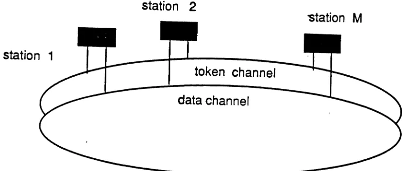
passing. In order to achieve this concurrence we have to move the control signals, the
control token, from the datachannel and permit another medium to carry it. Therefore,
we propose a dual-bus network which consists of one datachannel and one token
chan-nel. The data channel is a high transmission capacity medium used by data information
and the token channel isa lower bandwidth channel used to accommodate the system
sig-nalings in order not to interfere with the data information. This isthe basic idea behind
accesses to the data channel by the control token in the token channel.
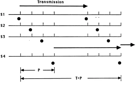
With C-token protocol, we can obtain a fairer scheduling and reduce the logical
dis-tance between two consecutive stations. Refer to Figure 1;S1and S4 are the two active
stations at the concurrent slot. S4 needs to wait a transmission time and a propagation
delay to start its transmission according to the type II token ring protocol. However, it
only takes a transmission time, assuming that transmission time isgreater than the
propa-gation delay between S1and S4, ifC-token protocol is used. Therefore, a smaller
possi-bility isachieved in C-token protocol for S2 and S3to generate packets and use the token
before S4. Furthermore, application of clear channel technique simplifies the operations
needed at the nodes since we separate the control signals and data information in two
Figure 1. Comparisons of token passing for tow different protocols.
2. THE MODEL AND PROTOCOL OF THE C-TOKEN BUS
A dual-bus networkwith M stations has amainchannel to carry data packets and a
token subchannel. Both channels are assumed to be time slottedwithslot size, t,equal to
the average propagation delay between any two consecutive nodes in the passing list.
This is distinct with the common assumption made in conventional slotted system in
which 't is equal to a round trip propagation delay. The stations are synchronized and
enforced to start transmission at the beginning of a time slot. As in the IEEE token bus
access to the data channel; only one user can access the data channel at any time. This
assumption conserves the conflict-free character of the protocol.
We study the model under the typical assumption [6] that each station will generate
8 new packet with a constant probability, 0, during a time slot. Once it generates a
packet, the packet will be stored in the station buffer until it is successfully transmitted.
While in this waiting state, the station is considered to be a backlogged station and no
longer generates packets. The channels are assumed to be error-free. The protocol is
described as follows:
[a] The backlogged stations have to wait for the token and listen to the data channel
when the token is received. If the data channel is sensed busy, the station will
keep the token and persists until the data channel becomes idle.
[b] Once the station which possesses the token finds the data channel idle it starts the
transmitting on the data channel.
[c] One time slot after the beginning of the transmission, the station releases the
token to the next station on the token channel. This ensures that the rest of
sta-tions are aware of the activity on the data channel.
[d] An idle station which receives the token simply passes it to the next station.
For a network as described above each station may be viewed as in Figure 3.2.
Bach station has two taps, a writing tap on the data channel and a token-receiving tap on
the token channel. Here, we assume that any delay caused by software or hardwarein the
another station.
station
2
station
1
data channel
statlon M
Figure 2. Configuration of a C-token ring local area network
3. ANALYSIS
The behavior of the system can bedescribedby a cycle period which consists of an
idle period and a busy period, Figure 2. An idle periodisdefined when no station in the
system is transmitting; there may be some backlogged stations but none of them are
allowed to send messages. A busy period means that the data channel isbeing used. Due
to the protocol we proposed and the evolution of the number of the backlogged stations
in the system, we can determine the stationary probability of the number of backlogged
BP
IP
BP
IP-.J_ _
--a...--_~
_ _ ' _ __ _Figure 3. Periodic behavior of the data channel
We assume that total number of stations in the networkisless or equal to the packet
size in term of slots in 3.1 and 3.2. According to the protocol, the transmitting station
releases the token one time slot after the beginning of the transmission, therefore, there
are surely no backlogged stations in the system when the last transmission station in a
busy period releases the control token. On the other hand, if there is any station in an
active state when the token isreleased, one of them will receive the token before the
ter-mination of the current transmission and starts another transmission. In this case the busy
period will continue, and the current transmitting station is not the last station that sends
packet in..the busy period. Based uponthis argument we derive an expression for the
dis-tribution of backlogged stations at the beginning of an idle period.
A similar technique is used to derive the distribution of backlogged stations at the
'e :
beginning of the firstslot of an idle period.I :length ofan idle period measured inslots.
N' : number of backlogged stationsinthe system at the beginning ofr,h slot.
T : fixed packet size measuredin slots.
M : number of stationsinthe system.
(J : probability for an idle station to generate a packet in a time slot.
Xi: probability of i backlogged stations in the system at time t,
•
Xi: probability of i backlogged stations in the system at one time slot after the
begin-ning ofabusy period.
The assumption, T ~M, may not be valid if the transmission speed of the data
channel increases on the number of station goes up. Therefore, weprovide the analysis
for T
<
M in 3.2. In this section the calculations for the distribution of the number ofbacklogged stations at the beginning of a busy period and an idle period are obtained.
The average length of a busy period and an idle period are given in section 3.3 such that
we can compute the system throughput. In section 3.4 the average backlogged station in
the system is analyzed such that we canuse Little's result to obtain the average waiting
time fora packetina node.
3.1. THE DISTRIBUTION OF BACKLOGGED STATIONS AT
t, FOR T
~MWithout loss of generality, the stations are named 1 to M according to the token
passing sequence. Thus station 1 passes the token to station 2 and station 2 passes to
sta-tion 3, and so on. Finally, stasta-tion M passes the token to station 1 and the passing
a particular busy period, then, at the moment when station 1 releases the token the other
M-1 stations must be in the idle state; there are no backlogged stations in the system.
For the given condition that station 1isthe one to end the busy period the number of time
slots in which the rest of the stations, stations 2 to M, can generate new packets is
(T+l-j) mod M according to their number respectively, j=2,..,M. Due to the
assump-tion ofT ~M ,we develop two expressions for the computation of the distribution of the
number of backlogged stations at the beginning ofan idle period.
CASE I :T isa multiple ofM
M-l
no
=
n
(I--<:J)(T-j)mod M j=l7t/:AFLfll1-(l-<J)(T-i.>mod
MMit
(l-<J)(T-i/J>modM)
E, 0=1 b=1+1
iQ , ib
e
(1,2, ...,M -1)(I)
(2)
E, is any combination ofI stations chosen from stations 2 to M. Inthis case,
it isnot possible for station 1 to be a backlogged station at t,
CASE
n :
T isnot a multiple ofMM-l
no
=
(1-<1)n
(l-a)(T-j)modM j-Ift,..o=<l-<J){ 'ltl E
case
I }+o{ 1t'-le
case
11 }(3)
(4)
In this case, station 1, which is
assumed
to initiate the busy period, returns to an idle stateThe proof of the derivation ofttl is straightforward but the numerical computation
requires some precaution (an explicit calculation seems to be hopeless). To overcome
this nwnerical difficulty, we present a convolution type algoritlun [7] in Appendix A for
the computation ofttl'so The proposed algoritlun has a complexity ofO(M2). The proof
of
'to
isbased upon the argument that given a busy period will be terminated by station I,the nwnber of slots during which station j, j=2, 3,...,M,may generate a new packet and
become an active station is (T
+
1-j )mod M. Therefore the probability that station jdoes not generate a new packetin this period is (l~)(T+l-j)modM, i.e.(1-a)(T-j) mod M,
for j=1,2,...
,M
-1. The expression for 1t/ l~, can be obtained by a similar argumentthat probability for stations 2 to M to become an backlogged station at the end of a busy
period, the beginning of an idle period, is 1-(1~)(T - j )mod M. Therefore, the probability
ofI stations become backlogged during this periodisexpressed by(2).
For case I,.T is a multiple of M , the beginning of the last slot of a busy period,
sta-tion M sends the token back to stasta-tion 1 which is the station initiates the busy period.
Station 1 does not have any possibility to become a backlogged station under the
assump-tion thatthis busy period will beterminated. In case Il,T isnot a multiple ofM ,station 1
returns to an idle state at the beginning of the last slot such that itcan be one of the
possi-ble candidates to be a backlogged station in a time slot. That is the reason 1-0 and
a
shown in(4) to represent the probability that station 1 does or does not generate a new
packet in one time slot.
3.1.1. THE BACKLOG DISTRIBUTION,ft/·,ATte+/
Consider a particular cycle, see Figure 4, which consists with an idle period starting
beginning of a busy period depends on the number of backlogged stations at the
begin-ning of the previous idle period and new arrivals at those stations which are in idle states
during this period. The token isreleased at t, and starts an idle period; from this point,
the token is passed station by station until an active station is found and a new busy
period starts. The computation of the distribution isbased upon the transition probability
of these two special time instants. The active station who will initiate a new busy period
can be either an old backlogged station or a newly generated backlogged station. An old
backlogged station means that it already had a packet waiting for transmission at time fe .
A newly backlogged station is a station that was idle atte and a new packet is generated
at the station during the idle period. Thus, the number of backlogged stations at t~+/ ,the
beginning of a busy period, must be greater than or equal to one less than the number of
backlogged stations at te depending upon whether the station which starts the busy
period is a newly backlogged station or an old backlogged station.
busy period
t
e
idle period
)(
t*
busy period
The notation that isusedinthe derivationisas follows;
P
I.s+1,n : probability of havings
backlogged stationsinthe system at t~ ands
+/back-logged stations at t~+/ given that a newly generated backlogged station
starts the busy period, whereI ~
o.
ps,s+1,0 : similar to the above except that an old backlogged station starts the busy
II:
newly backlogged stations who have been visited by the token during the idleperiod.
12: newly backlogged stations which have never been visited by the token during
the idle period.
where
{
/1+/ 2=1 I~1
/ 1=12=0 1=-lor 0
For the case ofS¢O,we easilyobtain
M-i-l
M-s-I ( )
s
. .
i-I ,, .,
+1Ps,s+I.n= I: M- (l-(l~)')n(1~Y I: I:n[l-(l~)· ]
; =1 ( 1) j=1 1=1\+12 E, •.;a=1
S
n
(l~);,,+I(M -~-;-1)[1_(l~i+I]'2(1~)(;+I)(M-s-i-12-1)
b=l1+1 2
where I: represents any possible combination of (/1,/ 2 ) with11+/z=1
'-1
1+12(5)
(6)
E'I; represents any possible set of
11
new backlogged stations from those i stations. Eachstation isindexed by a numberfrom 1 to i and station j , j
=
1...i ,can generate a packet inI
1:
n
[1-(1-<J);·+I]n
(1-<J);b+1 E,,,,a=l b=ll+1For the case ofs=O,we need one more step to compute the transition probabilities,
P,=0,1 ," andP,=lJJ,0· Consider an idle period that starts with no backlogged stations in
the system. We release the token and observe the number of backlogged stations in the
system at the beginning of each slot. Once the number of backlogged stations is no
longer zero then, we mark the time instant as
t;.
Dearly there are no backlogged stations in the system at the beginning of slot (;-1,
N,;-l=o. We definepj= P{ N':=j IN,;-I=o , j=l.M). Obviously, those j backlogged
stations mustbegenerated during the (t;_l)th slot. The probability of generating j
back-logged stations in one slot canbeexpressed as:
Therefore,
p
j. can be expressed as:We have
~
__ (M.~j
(l-ofl-
j , • 1 MP
J ) IV1-(1-0'1'
}
=..
·
(7)
The transition probabilities, P{N': =s I Nt.+I=s+l}, which are denoted by
P1,,1+1,11• andp.1,8,D+I for a new and an old backlogged station respectively can be obtained
n
(l--<J);h+1(M-~-i
-I )[I_(l--<J);+1]'2(l--<J)(i+l)(M-s-i-lrl)b-l1+1 2
n
(l--<J);6 +l(Mis-i)[I-(l--<Ji+1]1 2(l-(J)U+l)(M-s-;-I2)b=ll+l 2
(8)
(9)
Therefore the distribution of the number of backlogged stations at the beginning of a
busyperiod, denoted by1t;.,canbeobtained from;
• ;+1 • • ;+1
Xi
=
~ 7toPj Pj,;+~ 1tk Pic,; ,OSis
M -1 ·j=1 k=1
where
• •
•
P
j,i=P
j ,i,n+
P
j ,i,03.2. FOR THE CASE OF T
<M
(10)
In3.1 we analyze the system that the packet transmission timein slotsisbigger than
the number of stationsin the system such that the token can search allthe stations in the
network in a transmission time. Therefore we have a determinable point which has been
used to calculate the distribution of the backlogged station at the beginning of an idle
We have exact information of the system at this point; all the stations in the network
must be in idle states, otherwise, the busy period will not stop.
The assumption above will not be validifthe transmission speed of the data channel
increases to a certain degree such that token can not visit all the stations within a
transmission time. In this case, T<M , no such time instant we can use to analyze the
system. If we investigate a system of a busy period, the time instants that a transmitting
station releases the token, one time slot after its transmission, can be recognized as the
regeneration points in the busy period. The probability distribution of the backlogged
stations at those points are identical from which onward to the future of the evolution of
the number of backlogged stations is a probabilistic replica of the previous one. Such
characteristic canbeused to obtain the distribution of backlogged stations at those
regen-eration points. The distribution of backlogged stations at one time slot after the beginning
of a busy period,
1tt,
isconsidered tobeidentical to the distributions at any other point inthe same busy period.
We will analyze the behavior of the system in the busy period such that all
con-siderations of the analysis is based upon the given condition that all events are in the
same busyperiod. The conditional transition probabilitiesqij's are defined asthe
proba-bility that a transmitting station releases the token with i backlogged stations in the
sys-tem and j backlogged stations in the system when the next transmitting station releases
the token which isT
+
1 slots after the previous event. Obviously, the given condition isthat token must find an active station within T time slots in order to be able to continue
We obtain the qij as follows;
n
(1-(1);" +1(M-~
-i-I )[l-(I-(1i+1]\1-(1)(; +lXM-s-i-lr 1)b=11+1 2
1
n
(l-(1);,,+I(M-~
-i-I )[I-(l-(1i+1)'2(1-(1)0+IXM-s-i-lr 1)b=ll+1 2
M-i-l
T ( s 1 ) · ; - 1 .
'I
·
+1+
~-
[l-(l-a)'In
(l-a)' ~ ~n
[l-(l-a)'·l
"1 M -1 " 1 " "_. +I E 1
II: ( ) J= J-f=C1 2
'.J
Q=S
(12)
where ~ represents any possible combination of('1 ,/2 ) with 11+/2
=
j -i ,however,j-i=l1+/2
The definition of
E,,,i
isthe same as in 3.1.The first term in (12) represents the condition that the next transmission station is a new
backlogged station and the condition of a old backlogged station transmitting next is
represented in the second term. The consideration ofqij is similar to the derivation of
(5)(6).
Now, the balance equations for the regeneration points in the busy period can be
expressed as follows;
Inmatrix fonn we have
then,
n'
canbe obtain."+1 'It:= ~'It;.qe
i=O
M-l
•
•
1tM-l= ~ 'It;qi M-l
i:()
(13)
(14)
Based upon the
xt
obtained in (14) we are able to calculate Xi; the distribution ofthe backlogged stations at the beginning of an idle period. Again, the transition
probabil-ity is calculated given that the transition will change the state of the system from busy
From now on we change the definition ofqij to the conditional probability that the
last transmitting stations releases the token with i backlogged stations in the system and
afterT slots of time no active stationisfound while j backlogged stations in the system.
Clearly, if i
>
M -T, the transition probability iszero since token will find an active sta-tion inT time slots with probability one.for i
<
M - T andi Sj .Then,
x"
can be obtained as follows;"
.
1t" = ~Xi qi"
;=0
(16)
The principle behind the derivation in this section is that the distributions of the
backlogged station at the regeneration points are identical. The first transmission in a
busy period is considered to be exactly the same as the rest of the regeneration points,
even though, the transitions into the states at this point are from an idle period. The same
consideration isused for the last transmission in the busy period even though the
transi-tions out from the statesat this point are notinthe busy period any more.
3.3. THROUGHPUT ANALYSIS
LetS be the stationary throughput of the channel, i.e.,S isdefined as the fraction of
channel time occupied by successful transmissions. A standard result from renewal
theory [8] tells us that S can be obtained as the ratio of time the channel iscarrying
Therefore, we have
M-l T ~ 7t~~
, ,
R·;=0
S M-l
1:
7t; I;+(T+l)7t;*R;;::()
(17)
where I; is the expected length of an idle period, given Nt,=; and R; is the expected
be f tran - - - b -00· , +1
num r 0 srrussions m a usy pen givenN' =;. These values are derived inthe
next section.
3.3.1. THE EXPECTED IDLE LENGTHt,
According to the number of backlogged stations at the beginning of an idle period,
we have two different sets of expressions forIk .
CASE I: k;eO
(18)
Since the number of the backlogged stations, k ,at
'e
isnot zero, the token will findan active station in at most M -k slots. This equation can be interpreted as follows; the
first part in the bracket represents an old backlogged station that terminates the idle
period while the second part represents the event that a new busyperiod is started by a
new backlogged station.
In this case, we need to add another period in which the number of backlogged
sta-lions in the system changes from zero to non-zero. This event follows the geometric
dis-tribution with parameter A=1-(I-a)M, the probability of at least one new packet has
been generated in the system during one time slot. The expected length ofthis period
1 can be expressed as M
-1-(1-0)
The expected length to reach the beginning of the next busy period, which is
denoted by
I;,
canbe obtained byM-i-l M-i-I
M-Ic ( k 1 )i-I ( k ) ; - 1 .
1;=
~.
-
n(1-ai+
[l-(l-ailn(1-a)l (19);=0
<kf)
j=l<kf)
j=lTherefore, the expected idle period given that there are zero backlogged stations at the
beginning of the idle period,IIc=O'canbe obtained as
1 M-I • •
Ik=o
= l-(l-att Ik~/kPk
3.3.2. C()MPUTATI()N OFR;
(20)
In order to calculate the number of successful transmissions,R;,in a busy period we
introduce a state descriptor
U
,m
,I) [7] which describes the system at the instant thetoken is released. The state descriptor can be interpreted as follows; stationj ,the station
which starts the
busy
period is named 1, releases the token in the mrh slot inthe currenttransmission and I backlogged stations existinthe system at this moment. We define the
variable
YU,m
,/)'s as the expected number of successful transmissions in the periodsystem at the moment that stationj releases the token such that I
e
{O,I,...,M-I} for j=Iand
e
(O,1,2...,M-2) forj~l. The variables Y's satisfy the following linear equationsY(j,m;tl,l)=
1:
Y(j+l,m',r'> P (j,m ,l)-+(j+l,m',r')I
m')'
Y(j,m=I,I)
=
1+1:
Y(j+l,m ',r') P ( j,1,l)-+(j+l,m',r'>J
m')'
(21)
(22)
where P( j,m.l)-+(j+1,m',1'») represents the transition probabilities between two
con-secutive observed points at which the system is in states (j,m ,I) and
U
+
I,m',I')respec-tively. We need Y(1, 1,1 )' s, for 1=0, 1,...,M-I. For stationary consideration Y's must be
independent of j. We write the linear equations inmatrix form as follows:
where
Y(l,O) Y(I,I)
10
Y(I,M-l) II
Y(2,O)
12Y = Y(2,M-2) D =
1M -I
(23)
°
Y(T ,0)
T(T ,1)
°
Y(T ,M-2)
The transition
(U
,m,I)->U
,1,I')} indicates that the token is released when the stateof the system is
U
,m,I) and the next station which will receive the token happens to bean active station. Therefore, the token will bereleased in the next transmissionby station
j
+1; one time slot after the transmission. The components of the matrix B represent the
, ,
transition probability from state (m ,I) to state (m ,I ) associated with two consecutive
token releasing events. The sequence of the B matrix is the same as the Y matrix along
the row and the column dimension. The expressions for these elements are explicitly
given in Appendix B. Then, the Y matrix can be obtained from
(24)
Obviously, the information we want,
R;
's, are equal to Y(l,i)'s since we assume3.4. DELAY ANALYSIS
LetN bethe average channel backlog, obtained as the ratio of the expected sum of
backlogged stations over all slots in a cycle (average all cycles), to the average cycle
length. Therefore we have
where
M-l
1 • B
~
n·
B·+n·
B·~
"
"
N = ;=0
M-l[
1
;;.
n,
1; +7tt
R; (T+l)J(25)
B
f:
expected sum of backlogged stations over all slots in an idle period givenN '• ·=1.
B
f:
expected sum of backlogged stations over all the slots in a busy period givens':" ·
=1.The notation used in the following sectionissummarized as follows;
BKs+1•
$,0 • total number of backlogged stations over all the slots in an idle period, given
N'·=s, N'·-+!=s+l
andanold backlogged station starts the new busy period.BK:;/:
same definition as above except that a new backlogged station starts the busyperiod.
BK:;':
total number of bacldogged station over all the slots in the period between ,;isnot one of the backlogged stationsinthe system at
t;.
3.4.1. COMPUTATION OF
Bf
Consider an idle period with N"=s and
s':"
=s+l. The total number ofback-logged stations over all slotsinthis idle period can be categorized into two cases. Firstly,
it is an old backlogged stations that terminates the idle period. This implies 1+1
back-logged stations are newly generated in this idle period, then
n
(1~);,,+I(b;J
1+/2
b; )(M1:-i)[l_(l~);+I]\I~)(;+IX.M-S-i-12y.
b=ll+1
(26)
where
b
j is the expected number of slots that a new backlogged station isbacklogged inthe interval of length j slots given that the station becomes a new backlogged station in
this interval.
Or secondly, a newly backlogged station stops the idle period, in which case
we have,
n
(1~);.+l(6;J
1+/26;
)(M-~;i-l)[1-(1-<1);+1l'2(l-<1)(;+IX.M-.s-i-lrl)
For cases in which there are no backlogged stations in the system at time t~ we start counting the backlogged stations from
t;,
the time instant that the number of backloggedstations in the systemisnot zero. The equations are similar except that the lower limit of
the
first
summation starts ati
=
0 since the system may start a busy period immediately. Therefore the Bf
can be expressed asM-l
[M-l
M-l
~
B1
o
= ~ 1t. ~ BKs+1+
~ BKs+1~ I ~ 1,0 ~ S,"
3=1 1=-1 1=0
3.4.2. COMPUTATION OF
B{J
(28)
(29)
Let Z
U
,m,I) represent the expected number of backlogged stations in the system over all the slots in the period between the instant that the system is in the stateU
,m,I ) to the end of the busy period. Then, we also have a set of linear equations for the Z 's,ZU,m,I)
=
1+~
[K~)'+ZU+l,l/)]
P{(m,IH(1/)}(.:mtJX{I-ItO}
, ,
+
~ ZU+l,m+l,1 )P{(m ,l)--+(m+l,l )}(wruu{I-I,O)
(30)
The Z '8 are defined at the moment when the token is released such that the number of
time slots between two consecutive events will be either one or (T-1+m );the latter case
impliesthat the next stationisactive and it will holdthe token until one time slot after its
owntransmission.
K~1'represents the sum of backlogged stations over all the slots in the period we
at
the currentmth slot.
K Il 1(/-l)(T+1-m)
[(M,
-1-1)[I-(I-<J)T+2-m {+I-I (l-<J)(T+2-m)(M -(-2) (31)m,1 ~ /-/+1
[l_(I-<J)2][(l'-I)6'T+I-m +6'2]J
+
(~-l)
(1I (T+l-m) [(M-;1-2)[l_(l-<Jl+2-m{-I
(l-<J)(T+2-m)(M-t'-2)~ I-I
{
M - l if m=l '
where ~= M-2 if m~l ' (M-l)~1 ~max{l-l,O)
Theequation in matrix form is
Z=A
+
ZBThen
Z
=
A (I -B )-1where Bisthe transition matrix developedin3.3.2,
and
a(1,0) a(I,I)
a(M-I)
a(2,0)
where
A =
a(2,M-2)
a(T ,0)
a(T,M-l)
M-l
a(i,j)
=
I+
1:
K;~!P{(i,j)-+(l,k)}k=max(j-l,O}
(33)
(34)
Therefore we can obtainB! as Z(1,i).Finally, from Little's formula, the average packet
delay DELAY isgiven by
DELAY
=
N
S
4. NUMERICAL RESULTS AND DISCUSSION
From (24) (32) we know that the calculation of the analytical solution involves a
matrix with dimension T (M-1) x T (M-1) such that a small network is chosen as an
example to show the accuracyof the analytical solution in oder to avoid the computation
difficulties. The analytical solutionisverified bythe simulation resultsinFigure
S
and 6.The arrival rate in Figure S represents the probability thatan idle station will generate a
packet in a slot of time. According to the assumption that a backlogged station will not
maximum access delay can be calculated byDmax=(M -1)(T
+
1) andDmax is 60 slotsinthis case. We can see that
D
=60is the asymptote in Figure 5, at this moment all thesta-tions inthenetwork are busy at all time.
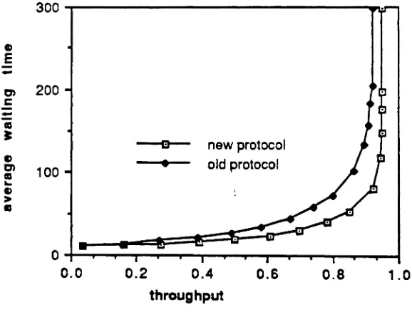
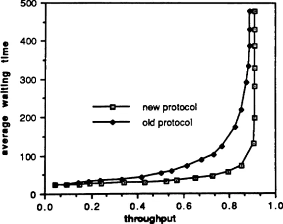
Figure 7 compares the performances of the new protocol with the conventional
token bus protocol by anetwork with20stations and T=20. We can see that the new
pro-tocol performs better thanthe old one does in any case. The relative improvement which
IDo -D" I
is calculated by % isshown in Figure 8. From Figure 8 we can see that the
Do
optimal operating point is at 0=0.015, at this point we can achieve 35% improvement
and the system throughput is about0.6.
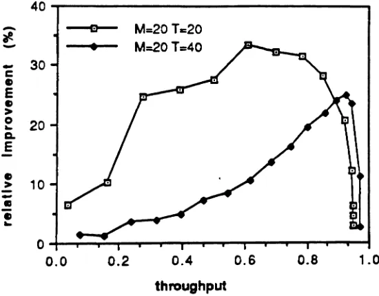
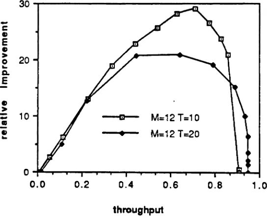
An important notice from Figure 9 is that a smaller packet size network is more
suitable thana system with larger packet size to implement the new protocol.InFigure 9,
for aM =20 network, T =20 obtains better improvement than the improvement that T =40
can obtain. This result canbe translated to that the new protocol will be agoodchoice for
the system which use higher transmission speed medium because the transmission time
of a packet will be shorter if a higher transmission speed medium is used. Figure 10
shows that a networkwill obtain better improvementifthe number of stations in the
net-work increases. This can be explained by the token passing time since at the same
throughput afewer population network has fewer number of token passing between two
active stations such that the relative improvement is not significant as a network with
larger number of stations.
By investigatingFigure 8, 9, 10 we can see that the new protocol obtain the optimal
a's
are different for different systems. And the throughput can be calculated roughly bythroughput
=
CJXMxT such that we can decide the optimal operating point for the newprotocol by controlling the
a's
for each station. The new double bus protocol is provedto perform better than the conventional single bus network, especially, for a high speed
local area network with larger number of stations.
Insection 3,we assume that the transmission time of a packet in slotsisbigger than
the number of stations in the network. This assumption simplifies the analysis
significantly, however, ifthe transmission capacity increases the transmission time of a
packet decreases then, this assumption is no longer valid. The results, refer to Figure 11
12 13, show that the conclusions made above is still hold. In such environment, type I
token ring protocol can only obtain throughput of 0.2 for a network M=49 T=10 based
upon the simple model developed in [11]. A remarkable improvement isachieved by the
1 .0 0.8 0.6 m analytical • simulation 0.2
O-l-...~...--r...,~r--....-~..,..-..,..--r-...,...,..~
0.0
new C-token protocol.
60 50 e E
...
40 en c=
II 30•
•
D) 20•
~ I) >•
1060 50 I) E 40
..
tn C 30..
CD ~ 20 I) tn CD a- 10 CD >•
0 0.0 0.2 m analytical • simulation 0.4 0.6 throughput 0.8 1.0Figure 6. Analytical and simulation comparison for M=6 T=lO.
300 I> E 0) 200 c :: CD ~ m new protocol I)
•
old protocoltn 100 CD a-Il > II 0
0.0 0.2 0.4 0.6 0.8 , .0
throughput
40
...
ae.~
..
c 30I) E I) > 0 20 ~ Q. E
•
> 100.001 0.002 0.003 0.004 0.005
throughput
Figure 8. Relative improvement on average waiting time forM=20 T=20.
40
... m M=20 TE:20
oe.
~
•
M=20 T=40...
30 c I) E•
> 0 20 ~ G. E e 10 >..
..
e ~ 00.0 0.2 0.4 0.6 0.8 , .0
throughput
40
.--... m M=20 T=40
-;ft
~
•
M=40 T=40..
c.,
30E I) > 0 20 a-Q. E
.,
> 10....
CD.,
a-00.0 0.2 0.4 0.6 0.8 , .0
throughput
Figure 10. Relative improvement on average waiting time for different number of stations.
m M=12 T=10 • M=12 T=20
30
....
c G) E I) > 20 0 a-Q. E.,
>-
10..
CD I) a-00.0 0.2 0.4 0.6 0.8 1.0
throughput
50 .-e 40 I) E t» > 0 30 ~ e, E
•
20 > .-.! I) EJ M=49T=10 ~ 10•
M=12T=10 00.0 0.2 0.4 0.6 0.8 1 .0
throughput
Figure 12. Relative improvement on average waiting time for different number of stations, a<
500
•
400 E..
at 300 c=
•
•
II new protocol•
200•
old protocolat
•
~•
>•
100 00.0 0.2 0.4 0.6 0.8 1.0
throughput
APPENDIX A
Computational algorithm forn1-eland Pj·(k)
n1=Lrl[(1_(l-es)(T-i&>modM]
i-Y
(1-es)(T-it ')modME,k=1 k'=I+l
"'-1
1 ~ (T-it')mod M
=Ln
[l_(l-es)(T-it )modM](1-est=l+lE,k=}
M(M-l) 1
=(1-es) 2
LO
[(1-es)-{T-it )modM-I] E,k=1Since,
M-l
L
(T-ik ,)mod M k'=1+1M-l 1
=L
(T-ik )mod M -L
(T-ik ,)mode Mk'=1 1'=1
And,
m
[(l-es)-{T-it)modM-I]E,k=!
M-I . M-l+l
=
L
[(I-<J)-{T-fl)modM-1].L
[(l-<J)-{T-iz)mod M-1]ifCl i~1+1
M-l
L
[(l-<J)-{T-iJ) mod M-I]iJ-=iJ-1+ 1
(A.I)
(A.2)
Define:
M-l
1:
[(l-<J)-{T-iJ )modM-I]iJ=fJ- 1+1
Forfixedj, j S M-l, we can design the recursive relation to obtainPj(k)'s:
Po(k)=l, forl Sk gf-l,
Pj(l)=[(l-<J)-{T-M+j)mod M-1]Pj-1(l),
Pj(k)=[(l-<J)-{T-M+j+A:-l)mod M-1]Pj_1(k }+Pj(k-I), for2 S;k S;M-j.
From the III can beobtained by
M(M-l)
III
=
(1-0) 2 P1(M-l), forl SISM-I.(A.4)
(A.5)
Asimilaralgorithm isdeveloped forthecomputation of
r,
n
[1-(1-0);1+1]n
(1-0);1+1E,.,;k=1 1=11+1
where
i
~ (;,+1) 11 •
=
r,
(1-o)b/,+\n
[1-(1-0)'1+1] E",;
1=1
; (; +3)
=
(1-0) 2r,
n
[(1-o)--{i1+l)_I]E",lk=1
Again we rewrite as follows;
;-11-1 ;-11 + 2 ;
= r,
[(l-o)--{i\+I)_I].r, .. , r,
[(l-o)--{;I,+I)-I]i1=1 iri1+1 ;',:;'r-l+1
Define:
(A.7)
(A.8)
;-1+1
P/*(k)= ~
i1'; -I -k +2
(A.9)
The following recursive relations can be used to obtainP,~(i -II) with a complexity of 0(;2).
P~(k)=l
P,~ (1)=[(l~)--{;-l\+2)-l]P'~_1(1)
P,~(k)=[(I~)--{i-l\~+3)_l]P/~_1(k )+p,~(k-I)
APPENDIX 8
Computation of the elements of the transition matrix B; P ((11,k )-.(/
2,m ) ) .
Define,
JM-I 11=1
1
M-2 If~1 and,~1
==
1-(I-o)T+2-m~2
==
(l-o)T+2-mPROPosmON B .1. -For the case, /2=/1+1.
P{(/I,k)--+(/1+l ,m )}
=(6-k)
e:
-I)0'"-.t (1-(Jt-m
~ m-k
B.I gives all the transitions for a station passing the token to an idle station.
PROPosmON B.2. -For the case, 12
=
1.P {(/I,k )-+(I,m)}
=(
1{
(1~~I)Pf-.t+lpt-'-1(1-(J)2-+{ ~=:)Pf-.tP~[l-(1-(J)2]}
(B.l)
(B.2)
PROOF. We assume that station 1is currently occupying the data channel such that the
station releases the token at IIdt slot is numbered by (/1modM). For simplicity we call
them stations
11
and /2·B.l represents the case that station 11 releases the token to the next station, 12 ,which is
M-k-I
of the remaining M -I-k idle stations ( probability ). m-k stations out of M-l
M -2-k idle stations will generate new packets during this time slot given station 12 is
still idle (probabilityisshowninthe remaining part of B.l ).
If station 11 is not the station that istransmitting , station 12 may be one of the idle
sta-M-2-k · al · · th h fir
tions with probability . The remamder of the an YSIS IS e same as t e s t M-2
case.
B.2 represents the cases that station/2iswaitingfor permission to transmit. Therefore
sta-tion /2 will hold the token until one time slot after its own transmission which is T +2-m slots
later.
There are two possibilities for station12needing tobeexamined; The firstpartin B.2 shows that
station 12has already backlogged atthe moment when station /1 is releasing the token; this
pro-bability is given by (.!). Then in order to satisfy the given transition I
+
I-k stations out ofl:1
fi-k stations in the system have to become backlogged in this period; this probability can be
obtained as
(/~k~I)~f+l-k~-l.
Since thestation who is cmrently occupying the datachan-Del will become idle T-m slots after the current slot, the probability for this station becoming a
backlogged station at the next token releasing time, T-m+2 slots after the current slot, is
(1-<1)2, 00 the other hand, the probability of the station not becoming a backlogged station is
1-(1-0)2.
Thesecond
pan
in B.2 showsthatstation12isDOtoneof the backlogged stations at the finttoken observed point suchthat it bastogenerate a new packetin this slot;the probability of satisfyingabove.
REFERENCES
[1] Werner Box, "Local-area subnetworks: A Performance Comparison," IEEE Trans. Com-mun., Vol. com-29, No. 10, Oct. 1981
[2] L. Kleinrock and F. A. Tobagi, "Packet Switching in Radio Channel: Part I - Carrier Sense Multiple Access Modes and their Throughput - Delay Characteristics," IEEE Trans. comm. Vol. com-23, No. 12, Dec. 1975
[3] A. G. Konbein and B. Meister, 'Waiting Line and Times in a System with Polling," J. of the Association for Computing Machinery, Vol. 21, No.3,pp470-490,July1974
[4] ANSI/IEEE standard Draft International Standard 802.4 - 1985 "Token Passing Bus Access Method"
[S] A.S.Taaenbaun. "Computer Network:' Prentice-Hall, Inc., 1981
[6] F. A. Tobagi and V. B. Hunt, " Performance Analysis of Carrier Sense Multiple Access with Collision Detection," Computer Networks4, No.5, 245-259
[7] P. Nain, N. D. Georganas,and W.
J.
Stewart, "Analysis ofaHybrid Multiple Access Pro-tocol with Free Access of New Arrivals During Conflict Resolution," IEEE Trans. Com-mun., vol. COM-36, No.7, July 1988.[8] Erbaneinlar,"lnttoduction to Stochastic Processes," Prentice-Hall, Inc., 1975
[9] L Cblamtac and A. Ganz, "Design and Analysis of Very High-Speed Network Architec-ture," IEEE Trans. comm., Vol. 36, No.3, March 1988.
[10] F. A. Tobagi and M. Fine, "Performance of unidirectional broadcast local areanetworks: ExptellnetandFunet," IEEE Trans. Select Areas Commun., Vol. SAC-I, pp 91-926, Nov. 1983.