Likelihood-Free Inference of Population Structure and Local Adaptation in a Bayesian Hierarchical Model

DOI: 10.1534/genetics.109.112391

Likelihood-Free Inference of Population Structure and Local Adaptation

in a Bayesian Hierarchical Model

Eric Bazin,*

,1

_{Kevin J. Dawson}

†

_{and Mark A. Beaumont*}

,2

*School of Biological Sciences, University of Reading, Whiteknights, Reading RG6 6BX, United Kingdom and†Rothamsted Research, Harpenden, Hertfordshire AL5 2JQ , United Kingdom

Manuscript received November 24, 2009 Accepted for publication March 29, 2010

ABSTRACT

We address the problem of finding evidence of natural selection from genetic data, accounting for the confounding effects of demographic history. In the absence of natural selection, gene genealogies should all be sampled from the same underlying distribution, often approximated by a coalescent model. Selection at a particular locus will lead to a modified genealogy, and this motivates a number of recent approaches for detecting the effects of natural selection in the genome as ‘‘outliers’’ under some models. The demographic history of a population affects the sampling distribution of genealogies, and therefore the observed genotypes and the classification of outliers. Since we cannot see genealogies directly, we have to infer them from the observed data under some model of mutation and demography. Thus the accuracy of an outlier-based approach depends to a greater or a lesser extent on the uncertainty about the demographic and mutational model. A natural modeling framework for this type of problem is provided by Bayesian hierarchical models, in which parameters, such as mutation rates and selection coefficients, are allowed to vary across loci. It has proved quite difficult computationally to implement fully probabilistic genealogical models with complex demographies, and this has motivated the development of approximations such as approximate Bayesian computation (ABC). In ABC the data are compressed into summary statistics, and computation of the likelihood function is replaced by simulation of data under the model. In a hierarchical setting one may be interested both in hyperparameters and parameters, and there may be very many of the latter—for example, in a genetic model, these may be parameters describing each of many loci or populations. This poses a problem for ABC in that one then requires summary statistics for each locus, which, if used naively, leads to a consequent difficulty in conditional density estimation. We develop a general method for applying ABC to Bayesian hierarchical models, and we apply it to detect microsatellite loci influenced by local selection. We demonstrate using receiver operating characteristic (ROC) analysis that this approach has comparable performance to a full-likelihood method and outperforms it when mutation rates are variable across loci.

T

HE study of the effects of natural selection at the genomic level has the potential to uncover hidden aspects of the causal pathways that relate genotype to phenotype and the environment (Sabetiet al. 2007). A challenge for any such research program is to dis-tinguish signals of selection from those of a myriad other processes (McVean and Spencer 2006), partic-ularly those related to the demographic history of the population. The study of individual candidate loci or regions of the genome, in isolation, and without regard to the (generally unknown) demographic history of the population is unlikely to be fruitful because selection can generally be mimicked by demographic processes

(Teshimaet al. 2006), and, indeed, this forms the basis of many methods of simulating loci under selection (Spencer and Coop 2004). As a consequence most recent studies concentrate on large-scale surveys of genomic regions, looking for genes that are discrepant (Teshimaet al. 2006). Within this framework there are two broad strands. One set of approaches is based around the idea of a ‘‘selective sweep’’ in which an allele increases in frequency, as a result of either a single novel mutation or a change in environment, leading to reduced diversity at linked sites (Kaplan et al. 1989). Another modeling framework is centered around the idea of ‘‘local selection’’ (Charlesworthet al.1997) in which alternative alleles are favored in different en-vironments. Unlike the selective-sweep scenario where the time of onset of the sweep is an important parameter, the local selection framework is essentially ahistorical: the allele frequencies within a deme are typically modeled by assuming migration–selection– drift balance (Wright1931; Petry1983).

Supporting information is available online athttp://www.genetics.org/

cgi/content/full/genetics.109.112391/DC1.

1_{Present address: Centre de Biologie et de Gestion des Populations} (CBGP), Campus International de Baillarguet, CS 30 016, 34988 Montferrier/Lez Cedex, France.

2_{Corresponding author: School of Biological Sciences, University of} Reading, Whiteknights, PO Box 68, Reading RG6 6BX, United

King-dom. E-mail: [email protected]

It is unclear at this stage which of the two forms of selection are most common. Certainly, the selective sweep scenario is commonly studied and this is unsur-prising because the two most intensely surveyed species, humans and Drosophila melanogaster, both have demo-graphic histories, the invasion of novel environments, that are conducive to selective sweeps. The model of local selection envisions a rather static view of the world, whereas the commonly held perception is of constantly changing environments and population restructuring. As always, probably the truth lies in between these two extremes, and the aim of this study is to continue the development of methods for detecting local selection, while recognizing the utility of the selective sweep par-adigm under many evolutionary scenarios.

Current methods of detecting local selection from gene-frequency information tend to be based around

FST, which has a variety of interpretations (Weir and

Hill2002; Balding2003). Here, it is defined to be the probability that two gene copies share a common an-cestor within the deme in which they are sampled without either of their lineages migrating (Crowand Kimura 1970, p. 105; Vitalis et al. 2001). Methods based onFSThave a long history (Cavalli-Sforza1966;

Lewontin and Krakauer 1973). The early methods were based on moment estimators ofFST, as in the above

two studies and also, for example, in Beaumont and Nichols(1996), Vitaliset al. (2001), and Weiret al. (2005). More recently, likelihood-based approaches

have been developed (Beaumontand Balding 2004;

Riebler et al. 2008; Foll and Gaggiotti 2008; Guo

et al. 2009). These latter approaches are based on a theory for the sampling distribution of genes in the infinite-island or continent-island model of structured populations. The same distribution, multinomial Di-richlet in form (a.k.a. Po´lya distribution or DiDi-richlet compound multinomial), can be derived either from the diffusion theory of Sewall Wright (Wright 1931; Rannala and Hartigan 1996) or from coalescent theory (Balding and Nichols 1994). The key insight that lies behind the use the multinomial-Dirichlet distribution in the detection of local selection is the following result. Marker loci, linked with recombination raterto loci in which locally deleterious alleles segregate with selection coefficients, have an effectively reduced migration rate,m, approximated in Petry(1983) asm9¼

m3r/(s1r) (Bartonand Bengtsson1986; C harles-worthet al. 1997). Under the structured coalescent with constant deme size and migration rates,FST ¼1/(11

2Nm), and hence under local selection there is expected to be heterogeneity in the estimates ofFSTamong loci.

The multinomial-Dirichlet framework has the advan-tage of having a simple likelihood function that is rapidly computed. If the mutation rate is low enough and the number of demes high enough, then we can justify this approach by the ‘‘many demes’’

approxima-tion of Wakeley (1998). Often this may not be an

adequate approximation, and the method then has the disadvantage that it assumes a simplified demographic history and cannot easily take into account recombina-tion and mutarecombina-tional processes. Given that likelihoods in more general frameworks are computationally in-tractable for large numbers of loci and recombination, it is tempting to consider using a likelihood-free approach (Pritchard et al. 1999; Beaumont et al. 2002; Marjoramet al. 2003; Becquetand Przeworski 2007). Typically these methods require that summary statistics are computed in a large number of Monte Carlo simulations and some match is made between simulated and observed summary statistics. A problem arises in that information on whether there is selec-tion comes from considering all the loci jointly, but to decide whether a specific locus is under selection we also need information on that particular locus. Thus a naive approach, given Lloci, would be to have Lsets of summary statistics. This could lead to thousands of summary statistics for an analysis. The probability of getting a close match for all L simulated loci will be vanishingly small, and consequently such an approach is unlikely to succeed.

In this article we develop a general method for efficiently computing solutions in hierarchical Bayesian models using a likelihood-free approach. We formulate a hierarchical Bayesian model for identifying loci that are subject to local selection and apply our technique, which is relatively efficient and easy to parallelize on a computing cluster. We demonstrate through the use of extensive comparisons that the method approaches the accuracy of the likelihood-based method of Beaumont and Balding (2004) in situations where the assump-tions of the latter hold and exceeds it when there is variability in mutation rate among genetic markers. We then apply the method to microsatellite data from chimpanzees.

A HIERARCHICAL APPROACH TO LIKELIHOOD-FREE INFERENCE

2009) and improved conditional density estimation (Blumand Francxois2009).

Briefly, we assume that we have measured a d

-dimensional vector of summary statistics S(x) from a data set. Here we make the distinction between the

observed data set x and the random variable, X,

generated by simulation. We haveNrandom draws of a (scalar) parameterFi(i¼1,. . .,N) and corresponding summary statisticsS(Xi) (i¼1,. . .,N) simulated from the joint distribution of parameters and summary statisticsP(S(X),F). (The model may have any number of parameters, which can be considered jointly, but the regression adjustment described here is applied to one parameter at a time.) We scaleS(x) andS(X) so that each summary statistic inS() has unit variance. We assume a linear model in which

Fi¼a1bTðSðXiÞ SðxÞÞ1ei;i¼1;. . .;N;

where theeiare drawn from a distribution common to all Xi, with a mean of zero. We use least squares to minimize

XN

i¼1

fF_iabT_ðSðX

iÞ SðxÞÞg2KeðkSðXiÞ SðxÞ kÞ; ð1Þ

where, assuming the model above,

a¼EðFjSðXÞ ¼SðxÞÞ;

kyk ¼

ffiffiffiffiffiffiffiffiffiffiffiffi Xd

i¼1 y_i2 v u u

t ;

with Epanechnikov kernel

KeðtÞ ¼ ce

1_{ð1 ðt=eÞ}2_{Þ t#e}

0 t.e:

ð2Þ

Given the estimates ˆa and ˆb, we can approximate posterior densities by using the assumption (above) that the distribution of errors is constant in the region whereKe(kS(Xi) –S(x)k) is positive and hence adjust the parameter values as

F*

i ¼FibˆTðSðXiÞ SðxÞÞ ð3Þ

(Beaumont et al. 2002). The posterior density for F can be approximated using some density estimation method, and in this article the local-likelihood method of Loader(1996) is used, implemented in Locfit under R, weighting the points withKe(kS(Xi) –S(x)k) as above. It should be noted that the ‘‘tolerance’’ of the method, as discussed in this article, is not measured directly in terms of the Epanechnikov bandwidthe, but in terms ofPe, the proportion of simulated points wherekS(Xi) –S(x)k#e. In the context of the ABC algorithm above the choice of summary statistics and the choice of metric (implicitly

Euclidean, in the example above through the use of the Epanechnikov kernel) are intertwined. Ideally one would choose summary statistics that are of low

di-mension and are also Bayes sufficient (Kolmogorov

1942). That is, we want the summary statistics S(x) to satisfy the condition

PðvjxÞ ¼PðvjSðxÞÞ ð4Þ

at all pointsvin the parameter space, for all priorsP(v) (so that we are free to choose whatever prior we want). In practice, such statistics are rarely available. Many approaches to ABC (Pritchardet al. 1999; Marjoram

et al. 2003; Sissonet al. 2007) are based on the idea of ‘‘rejection’’ (of observations falling outside a small ac-ceptance region centered on the observed data), giving

P(Fjr(S(X),S(x)),¼e) for some metricr(). Thus, particularly for high-dimensional S(), consideration should be given as much to the metric as to the summary statistics. Methods that place more emphasis on condi-tional density estimation (Beaumontet al. 2002; Blum and Francxois2009) aim to estimateP(FjS(X)¼S(x)) more precisely. A goal of such methods is to estimate the density using a larger proportion, possibly all, of the simulated points (Blumand Francxois2009).

Application of the ABC method to the situation addressed in the present study has a number of dif-ficulties. We wish to make inferences on the demo-graphic history and also on individual loci. This is a problem that is suited to a hierarchical Bayesian ap-proach, and the main contribution of this study is to devise a method for performing hierarchical Bayesian analysis in the likelihood-free framework. In simple models the parameters for each locus are assumed to be identical, and if a likelihood function is available, it is simply multiplied across loci. By contrast, taking muta-tion rate as an example, in a hierarchical model theL

loci each have their own parameter. At one extreme, identical to the simple case above, if the variability in mutation rate among loci is zero, then, in the terminol-ogy of hierarchical models, strength is ‘‘borrowed’’ completely between the loci, and each locus has an identical posterior distribution for mutation rate, and this is the same as the posterior distribution for the hyperparameter specifying the mean of the prior for each locus (the prior for each locus, having, in this case, zero variance). This verbal description is made clearer in the examples below. At the other extreme, the mutation rates at each locus are inferred independently—they have independent posterior distributions, and their prior has a high variance. More typically, the situation is intermediate.

and so forth. We refer to these as symmetric summary statistics. This is a typical use of the ABC method for data with many loci (e.g., Pritchard et al. 1999 and sub-sequent likelihood-free articles). The use of means and variances of summary statistics among loci for the ABC

analysis allows straightforward inference of the

hyperparameters.

By contrast, the focus of the present study is to make inferences on locus-specific parameters, as well as inferring the hyperparameters. This leads to difficulty because one needs summary statistics for each locus. The problem of a plethora of summary statistics has been noted in the Introduction. More fundamental is that, in the absence of missing data, the loci simulated under the model are exchangeable (their ordering or labeling is irrelevant to the likelihood). Thus there is no preferred ordering of the sample loci when compared with those generated by simulation. This problem is intrinsic to any hierarchically structured model and has been encountered before in an ABC setting by Hickerson et al. (2006) and Hickerson and Meyer (2008), in which the exchangeable units were taxa (rather than loci, as here). Since the ordering is arbitrary, a naive scheme would simply be to match the summary statistics of the first simulated locus with the those in the first data locus (given an arbitrarily chosen order) and so forth. Although correct in principle, such an approach would be hopelessly inefficient in practice in situations with many loci. Since the ordering is arbitrary, one might find a permutation of the simulated loci that gives the closest match. However, again, with many loci such a procedure is likely to be highly computer intensive, and, without exhaustive searching, not guaranteed to find the optimal match. The method proposed by Hickerson et al. (2006) was to rank the taxa by one of the key summary statistics, which makes the problem computationally tractable. However, there is then the problem of which summary statistic to use, and if the statistics are not strongly correlated it may not be very efficient. Similar issues have also been encoun-tered in Sousaet al. (2009).

Here our approach is to make use of locus-specific summary statistics together with symmetric summary statistics (those that are invariant to locus ordering) in a computationally efficient way, which we now describe. Suppose that we have a hierarchical model in which there areLloci. For the sake of example we concentrate on loci, but the argument can apply to populations or other repeated units. Each locus has a vector of observations (Xi) and (unobserved) parameter vectors kiandli(i¼1,. . .,L). Here, we treatlias a parameter of interest andkias a nuisance parameter. We make this distinction for ease of exposition: it is not fundamental to the treatment below. We assume the vectorli is of

relatively low dimension, while k_i may be of high

dimension. Letk¼(k1,. . .,kL) andl¼(l1,. . .,lL).

The likelihood function for our model is

PðXjk;lÞ ¼ Y L

i¼1

PðXijki;liÞ

" #

; ð5Þ

whereX¼(X1,. . .,XL). We assume that, conditional on the hyperparameter a, the priors for each locus are independent, and so

Pðk;ljaÞ ¼Y L

i¼1

Pðk_i;l_ijaÞ: ð6Þ

Thus the joint prior densityP(a,k,l) is

Pða;k;lÞ ¼ Y L

i¼1

Pðki;lijaÞ

" #

PðaÞ; ð7Þ

with a prior (hyperprior)P(a). Because of conditional independence, it is straightforward to show (appendix) that the joint posterior density can be factorized as

Pða;k;ljXÞ ¼ Y L

i¼1

Pðk_i;l_ijXi;aÞ

" #

PðajXÞ; ð8Þ

or, marginal to the nuisance parameterk,

Pða;ljXÞ ¼ Y L

i¼1

Pðl_ijXi;aÞ

" #

PðajXÞ: ð9Þ

Focusing out attention on a single locus i, the hyper-parametera and the locus-specific parameter li have the joint density

Pða;lijXÞ ¼PðlijXi;aÞPðajXÞ: ð10Þ

This factorization suggests that we need to use two distinct types of summary statistics in our approximate Bayesian computation: symmetric summary statistics, which are functions of all the loci together (e.g., means, higher moments,. . .), S(X) ¼ S(X1,. . ., XL);

and unit-specific summary statistics, U(Xi). Rather than insisting that the complete set of summary statis-tics is Bayes sufficient (see Equation 4), we can now make do with the weaker requirement that S(X) and

U(Xi) satisfy

Pða;lijXÞ ¼PðlijUðXiÞ;aÞPðajSðXÞÞ; ð11Þ

at all points (a,li) for the chosen prior (or family of priors). We want this to hold exactly or at least as an

adequate approximation. In the terminology of

Algorithm 1:

1. Fork¼1 tok¼Niterations:

i. Sample (Ak, Kk, Lk) from the prior P(k, l j

a)P(a).

ii. Simulate dataXk(atLloci) fromP(XkjKk,Lk). iii. For locusi¼1 toi¼LcomputeU(Xk, i).

iv. ComputeS(Xk).

2. Use ABC to condition on S(X) ¼ S(x) (approxi-mately) to obtain a sample of observations A* from

P(ajS(x)) (marginal tok,l). 3. For locusi¼1 toi¼L:

Use ABC to condition on S(X)¼S(x) and U(Xi)¼

U(xi) (approximately) to obtain a sample of observa-tionsL* fromi P(li,jS(x),U(xi)) (marginal toa,k).

Providing the summary statistics are sufficient, and in the limit that the ABC tolerance e/0, this algorithm should sample from the posterior distribution (9) above without additional approximation. There is, however, a practical problem of computer storage associated with this algorithm. If there areusummary statistics inU(Xi), we would need to storeNLuitems. For example, with 103_loci,

10 summary statistics per locus, 106_{iterations, and 8 bytes}

per number, we would have 80 Gb of storage as a binary file or in computer memory—much larger, if stored as text files. Thus, although the algorithm may work well with smaller problems there is a generic problem in scaling up. The second algorithm is similar to sequential ABC algorithms (Sissonet al. 2007; Beaumontet al. 2009) in which the problem is attacked in two bites.

Algorithm 2:

Step 1. Fork¼1 tok¼Niterations:

i. Sample (Ak, Kk, Lk) from the prior P(k, l j

a)P(a).

ii. Simulate dataXk(atLloci) fromP(XkjKk,Lk). iii. ComputeS(Xk).

Condition on S(X) ¼ S(x) using ABC, to obtain a sample of observationsA* from

PðajSðxÞÞ PðajxÞ:

Step 2. For locusi¼1 toi¼L: Fork¼1 tok¼Niterations:

i. SampleAk** fromP(ajS(x))P(ajx) by resam-pling from the observationsA* generated in step 1. ii. Sample ðKk;i**;Lk;i**Þ from the conditional

priorP(ki,lijAk**).

iii. Simulate data Xk,i (at locus i only) from P(Xk,i

jKk;i**;Lk;i**). iv. ComputeU(Xk,i).

Condition onU(Xi)¼U(xi) using ABC, to obtain a sample of observations (A***, Li***) from an approxi-mationtoP(l_ijxi,a)P(ajx).

Note that in step 2 above, if sample sizes are identical at each locus (no missing data), then it is necessary to iterate only for one locus, rather than for locusi¼1 to

i¼L, because the distribution is the same. The advan-tage of Algorithm 2 over Algorithm 1 is that it scales easily with increasing numbers of loci. The amount of storage is 1/L less than Algorithm 1. The time cost of Algorithm 2 is potentially twice as high, but for, e.g., simulated data or data with equal sample size at each locus it is of the same order as that of Algorithm 1. With a computing cluster of many nodes, the overall execu-tion time may be quite low because step 2 in Algorithm 2 can be performed independently for each locus. An additional advantage is that in the second round of

simulation the hyperparameter a is already sampled

from an approximation to the posterior distribution, and therefore, as with sequential methods (Sissonet al. 2007; Beaumontet al. 2009; Toniet al. 2009), there is a potential for increased precision in our approximation to the posterior distribution of li, ameliorating that apparent inefficiency of having a second round of simulation. However, a key point to note is that Algorithm 2, in contrast to Algorithm 1, involves an approximation that is in addition to that arising from the use of summary statistics that do not satisfy the marginal sufficiency conditions in (11) and nonzero tolerancee.

To simplify the explanation of this additional approx-imation, we assume that we are performing ABC on complete data and that, by whatever means, we can sampleafrom the true posterior distribution. Then in the two-step algorithm, after step 1, we have a sample from

Pðl_ijaÞPðajX ¼xÞ

(marginal to ki), where X9_i is the random variable corresponding to the data simulated in the second round. Using ABC we then condition onX_i9¼xi. This gives us a sample of observations (A***,Li***) from

PðXi9¼xi;lijaÞPðajX ¼xÞ PðX9_i¼xijX ¼xÞ

;

which is not the same as the desired posterior density

P(li,ajX¼x).

By contrast, consider a modification of the two-step algorithm, where we sample fromP(ajX–i¼x–i) at step

1 [instead ofP(ajX¼x)]. (The subscript –iindicates all the data except that from locusi.) Now we have a sample from

PðXi;lijaÞPðajXi ¼xiÞ:

PðXi¼xi;lijaÞPðajXi¼xiÞ PðXi¼xijXi¼xiÞ ¼Pð

l_i;ajX ¼xÞ

because

Pðxi;lijaÞPðajxiÞ PðxijxiÞ

¼Pðxi;lijaÞ PðxijaÞ

PðxijaÞPðajxiÞ PðxijxiÞ

¼Pðxi;lijaÞ PðxijaÞ

Pðxi;ajxiÞ PðxijxiÞ ¼Pðl_ijxi;aÞPðajxi;xiÞ ¼Pðl_ijx;aÞPðajxÞ ¼Pðli;ajxÞ:

When the number of lociLis large, we then expect that any one locusi will make an almost negligible contri-bution to the information about the hyperparametera, so that

PðajxiÞ Pðajxi;xiÞ ¼PðajxÞ:

Therefore, in this case our two-step algorithm should differ very little from the modified algorithm that can be demonstrated to provide samples from the correct posterior distribution (with ABC error).

APPLICATION TO GENE FREQUENCY DATA

The model: The primary aim of this study was to model local selection and compare the results of the ABC algorithm with the Bayesian method of Beaumont and Balding(2004), which uses an explicit multinomial-Dirichlet function for the likelihood. We wished to investigate the relative efficiency of both methods, using receiver operating characteristic (ROC) analysis. In one case microsatellite data are simulated with low variation in mutation rate among loci, and in the other it is high. It is expected that the multinomial-Dirichlet likelihood will behave poorly in the latter case because it assumes that all genetic variation is ancestral (i.e., it arises in the ‘‘collecting phase’’ of Wakeley1998). To keep the mod-els similar, we assume an island model. The multinomial

Dirichlet arises under an infinite-island or continent-island case (Baldingand Nichols1994; Rannalaand Hartigan 1996), but it is pragmatically easier for the ABC analysis to assume a finite number of demes equal

to the number of samples. Unlike Beaumont and

Balding (2004) we consider only a model in which positive local selection is modeled.

Variation in mutation rate and migration rate is modeled in a hierarchical Bayesian framework,

simi-lar in conception to that described in Storz and

Beaumont(2002). We assume that there areDdemes. The scaled mutation rate at theith locus isu_i¼2Nm_i, whereNis the haploid effective size of the deme andm_i is the mutation rate at theith locus. The scaled mutation rate, ui, has a prior that is a log10-normal distribution

with (on a log10scale) meanmuand standard deviation su. We use a Gaussian hyperprior formuand a truncated

Gaussian forsu(Table 1). Note that we do not use an

inverse gamma for thesu, following the

recommenda-tion of Gelman (2006). Variation among loci in

migration rate is modeled in a somewhat different way. The principal idea is that there is an indicatorZi that takes the value 0 if theith locus is ‘neutral’ and 1 if it is subject to local selection. The prior for this is Bernoulli with probabilityr_Zthat the locus is under selection—i.e., the prior expected number of loci under selection is

LrZ. The hyperprior forr_Zis beta with parameters given in Table 1. Using the approximation of Petry(1983) that local selection acts to reduce the apparent migra-tion rate, we assume that theith locus and thejth deme have scaled migration rateMij¼2Nmij, where

Mij¼

Nj ifZi¼0

Sij ifZi¼1:

The neutral migration rate varies among demes with a log10-normal prior having (on a log10scale) meanmM

and standard deviation sM, with Gaussian hyperprior

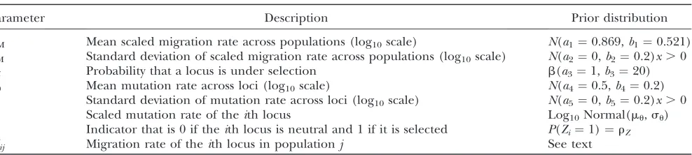
(Table 1). Note that since we have a constantuacross demes, we implicitly assume that variation inMnacross demes is through m and N is constant. For local dir-ectional selection we assume thatSijhas a prior given by TABLE 1

Model parameters and their prior specification

Parameter Description Prior distribution

mM Mean scaled migration rate across populations (log10scale) N(a1¼0.869,b1¼0.521)

s_M Standard deviation of scaled migration rate across populations (log10scale) N(a2¼0,b2¼0.2)x.0

rZ Probability that a locus is under selection b(a3¼1,b3¼20)

mu Mean mutation rate across loci (log10scale) N(a4¼0.5,b4¼0.2)

su Standard deviation of mutation rate across loci (log10scale) N(a5¼0,b5¼0.2)x.0

ui Scaled mutation rate of theith locus Log10Normal(mu,su)

Zi Indicator that is 0 if theith locus is neutral and 1 if it is selected P(Zi¼1)¼rZ

Mij Migration rate of theith locus in populationj See text

a scaled beta distribution with density bðx=Nj;1; 15Þ=Nj. Thus, for a locus under local directional selection the prior migration rate has a maximum equal to the neutral migration rate, but is more heavily weighted toward lower values. The directed acyclic graph (DAG) for this model is given in Figure 1.

In all our examples below, the point values chosen for the parameters of the hyperpriors,a1,. . .,a6,b1,. . .,b6,

are given in Table 1.

The likelihood function for our model has the form

PðXjl;aÞ ¼Y L

i¼1

PðXijli;aÞ; ð12Þ

where here we implicitly marginalize over the nuisance parameter,k. HereX¼(X1,. . .,XL) withXi¼(Xi1,. . .,

XiD), and a¼ ðN1;. . .;ND;rZ;mM;sM;mu;suÞ. The

locus-specific parameters areli¼(ui,Mi1,. . .,MiD,Zi).

The joint priorP(l,a) factorizes as in (7). The factor

P(a) (the hyperprior) is now of the form

PðaÞ ¼ Y j

PðNjjmM;sMÞ

" #

Pðm_M;a1;b1ÞPðsM;a2;b2Þ Pðr_Z;a3;b3ÞPðm_u;a4;b4ÞPðsu;a5;b5Þ;

ð13Þ

and each factorP(lija), of the prior density, is of the form

Pðl_ijaÞ ¼ Y j

PðMijjZi;Nj;a6;b6Þ

" #

PðZijrZÞ

Pðu_ijm_u;suÞ: ð14Þ

Each factorP(Xijli) of the likelihood function is of the form

PðXijliÞ ¼ Y

j

PðXijjui;MijÞ: ð15Þ

For a model of this form, with this choice of prior, the marginal posterior densityP(a,ljX) has a factorization of the form (9), in whichaandl_iare replaced by the pa-rameters of our genetic model, as specified above. Hence our model is amenable to the use of Algorithms 1 and 2. Summary statistics:The main aim of the model is to characterize the level of genetic differentiation between populations and differences among loci in their levels of differentiation and genetic variability. The choice of summary statistics has then been based on earlier work relating the expected value of summary statistics to demographic parameters and also to work that has used summary statistics of differentiation to identify loci that are potentially under selection (Beaumont and Nichols1996; Vitaliset al. 2001; Excoffieret al. 2009). The strategy has been to compute a set of locus-specific summary statistics U(Xi), and then, for the symmetric

summary statisticsS(X), the means and other moments of these statistics over loci have been computed.

Locus-specific summary statistics:For each locus we computed the following:

1. The observed probability of nonidentity in state of gene copies between populations,HB, computed as

in Beaumont and Nichols (1996), based on the estimator of Weirand Cockerham(1984).

2. The Weirand Cockerham(1984) estimator ofF_ST, computed as in Beaumontand Nichols(1996). 3. The logarithm of the variance in microsatellite length

between populations. The variance in microsatellite length between populations isSˆ3in Rousset(1996).

4. The statistic ˆr_ST of Rousset(1996), modified from Slatkin(1995), computed asðSˆ₃Sˆ₂Þ=Sˆ₃, whereSˆ₂ is the within-population variance in length, averaged over populations, without weighting for differences in sample size.

5. The variance in the Weirand Cockerham (1984)

estimator of FST estimated for individual alleles

(microsatellite lengths). In this case, a locus withKi alleles was converted intoKibiallelic loci with allele frequencies comprising those of the target allele and all the others combined.

6. In a K 3 Dtable of presence/absence of an allele (microsatellite length) in a population, the propor-tion of pairwise comparisons between populapropor-tions in which an allele is observed in at least one of the populations, averaged over alleles. This summary statistic has no previous theoretical basis, but was observed to reduce the mean square error of param-eter estimates in simulation tests.

7. The variance of the within-population Weir and Cockerham estimator ofFST(Weirand Hill2002), computed as in Vitaliset al. (2001).

8. The variance of within-population ˆr_ST computed analogously [i.e., as ðSˆ3Sˆ2jÞ=Sˆ3, whereSˆ2j is com-puted for each population rather than averaged].

Symmetric summary statistics: To infer hyperpara-meters we computed 60 symmetric summary statistics

S(X), invariant to locus ordering. These included the mean, variance, skew, and kurtosis over loci of the 8

summary statistics above, giving 4 8 ¼ 32 summary

statistics, and then the covariance over loci of all 28 pairs of summary statistics.

Transformation of symmetric summary statistics: Previous studies have suggested the use in ABC of transformations, including rotations of the summary statistics (Fagundeset al. 2007; Wegmannet al. 2009). Because a large number of summary statistics were used, we considered the use of orthogonal transformations of the data to reduce dimensionality. There appear to be two main issues. First, with a large number of summary statistics, many of which are uninformative, a large amount of ‘‘noise’’ is introduced into the computation of distance of simulated data from the observations. Essentially, summary statistics that are unaffected by the parameter values should be weighted out of the distance calculation (Hamiltonet al. 2005) or not chosen at all (Joyceand Marjoram2008). Second, there may be a problem of collinearity and resulting instability of the regression once many summary statistics are introduced. The use of partial least squares (PLS) in an ABC context has been suggested by Wegmannet al. (2009). With PLS the orthogonal axes are ordered by decreasing covariance with the independent variable, and it is often used in calibration problems (Gemperline 2007). In our two-step procedure, we need to sample parameters

from the joint posterior distribution of hyperpara-meters, which creates a difficulty because standard PLS assumes a univariate independent variable. A modifica-tion of the PLS algorithm exists (PLS-2) for use with a multivariate independent variable. However, we have chosen to use principal component analysis (PCA), also commonly used in calibration and typically producing

similar results (Mevik and Wehrens 2007), which

orders the axes by decreasing variance. A potential disadvantage of PCA is that axes with small eigenvalues may still have high correlation with the independent variable (here the parameter of interest). To take into account possible correlations between eigenvalues and independent variables, at least marginally, we have defined the following procedure:

The summary statistics sampled from the prior pre-dictive distribution were scaled to have unit variance and rotated (using the R packagePrcomp).

A Box–Cox transformation was then applied to the resulting eigenvectors.

These were then standardized once more to have unit variance and centered to have zero mean.

The Euclidean distance between these points and the target was computed.

On the basis of the 5% closest points, for the ith

component and jth parameter value, the squared

correlation coefficient r2

ij was computed. The

compo-nents were ranked by the proportion Rij¼rij2=

P

ir

2

ij. The set of ranked components in whichP_iRij$0:8 was retained, for each parameterj.

The union was formed over all parameters of the above sets.

The 30 components with the highest eigenvalue were then retained.

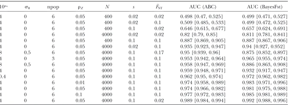
TABLE 2

AUC with 95% C.I. for ABC and BayesFst methods under different scenarios

10mu s

u npop rZ N s FST AUC (ABC) AUC (BayesFst)

4 0 6 0.05 400 0.02 0.02 0.498 [0.47, 0.525] 0.499 [0.471, 0.527]

4 0 6 0.05 400 0.02 0.1 0.509 [0.485, 0.533] 0.499 [0.472, 0.525]

4 0 6 0.05 400 0.1 0.02 0.646 [0.615, 0.677] 0.657 [0.624, 0.691]

4 0 6 0.05 4000 0.02 0.02 0.82 [0.79, 0.85] 0.811 [0.781, 0.841]

4 0 6 0.05 400 0.1 0.1 0.887 [0.869, 0.905] 0.887 [0.867, 0.906]

4 0 6 0.05 4000 0.02 0.1 0.935 [0.923, 0.947] 0.94 [0.927, 0.952]

8 0.5 6 0.05 4000 0.1 0.17 0.95 [0.939, 0.96] 0.875 [0.852, 0.897]

4 0 3 0.05 4000 0.1 0.1 0.953 [0.942, 0.964] 0.965 [0.955, 0.974]

8 0.5 6 0.05 4000 0.1 0.1 0.958 [0.947, 0.969] 0.886 [0.863, 0.908]

4 0 6 0.05 4000 0.1 0.1 0.959 [0.948, 0.971] 0.932 [0.917, 0.947]

0.4 0 6 0.05 4000 0.1 0.1 0.962 [0.95, 0.974] 0.972 [0.962, 0.982]

4 0 6 0.01 4000 0.1 0.1 0.974 [0.958, 0.989] 0.983 [0.971, 0.996]

4 0 6 0.05 4000 0.1 0.1 0.974 [0.966, 0.982] 0.981 [0.975, 0.988]

4 0 6 0.1 4000 0.1 0.1 0.977 [0.972, 0.983] 0.985 [0.981, 0.989]

4 0 6 0.05 4000 0.1 0.02 0.989 [0.984, 0.994] 0.992 [0.988, 0.996]

Nm, scaled mutation rate;sm, standard deviation of mutation rate across loci (on log10scale); npop, number of populations;rZ,

proportion of loci under selection;N, subpopulation size; s, selection coefficient. As noted in the text,FSTj for populationjis drawn

from a beta distribution with parameters (a¼_{FST =0:02,b¼ ð1FST Þ=0:02). The immigration rate,N}

jin the terminology of our

The regression-based ABC method was then applied (as outlined in Equations 1–3) withPe¼0.02.

No claim is made that the above procedure is optimal, and it was obtained through trial and error, on the basis of simulated data with known parameter values. A parti-cular feature of the approach is that there appears to be reduced sensitivity to the addition or removal of summary statistics. The locus-specific summary statistics were used in ABC regression without rotation or further transformation.

The algorithm: Our inference procedure is divided into two steps. We initially approximate the posterior distribution of the higher-level parameters usingS(X), and we then approximate the posterior distribution for locus-specific parameters usingU(X), as outlined in the following ABC algorithm, based on algorithm 2 above:

1. Compute symmetric summary statistics from the data.

2. Sample the following: a. rZ,mM,sM,mu,su;

b. ui,Zi,Nj; c. Mij.

3. Run a coalescent simulation of an island model (de-scribed in Beaumontand Nichols1996; Beaumont and Balding2004) to obtain data setsXij.

4. From the simulated data sets, compute the symmetric summary statistics from theXijin the same way as for step 1 above.

5. Return to step 2 untilnsets of summary statistics are obtained.

6. Perform regression ABC (as outlined in the pre-ceding section) to obtain Pen samples from the posterior distribution, wherePeis the proportion of points accepted.

7. For each locusi:

a. Compute locus-specific summary statistics from the data for this locus.

b. In the following order:

i. Sample with replacement from thePen sam-ples generated at step 6,rZ,mM,sM,mu,su.

ii. Sampleui,Zi.

iii. SampleNjforj¼1,. . .,D. iv. SampleMijforj¼1,. . .,D.

v. SampleXijforj¼1,. . .,D.

vi. Compute the locus-specific summary statistics as for step 7a above.

vii. Return to step 7b until n sets of summary statistics are obtained.

c. Perform ABC one locus at a time (this time measuring locus-specific summary statistics).

PERFORMANCE

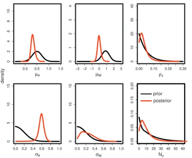
To examine the performance of the ABC approach we simulated groups of 100 data sets for 15 different combinations of parameters (scenarios), chosen to vary widely under the assumed prior (Table 1). An archive (suitable only for running on a cluster) containing source code, scripts, and input files for repeating and Figure2.—Posterior distribution of genome-wide parameters. The data set contains 100 loci and a sample of 100 gene copies

checking the results presented here is available at

http://www.rubic.reading.ac.uk/mab/stuff/ABCsims.

zip. These scenarios included selection coefficients of 0.02 and 0.1. We used ROC analysis, implemented in the ROCR package (Sing et al. 2005), as in Riebleret al. (2008), to compare the ABC method with BayesFst (Beaumontand Balding2004). In the case of the ABC method the classifying variable is the posterior proba-bility of locusibeing under selection,P(Zi¼1jU(Xi),

S(X)), while in the case of BayesFst it is a BayesianP -value (Beaumontand Balding2004). Specifically, for the case here, the P-value we use is the posterior probability that the locus effect,a, is less than or equal to zero and hence is a one-tailedP-value, for consistency with the ABC model, rather than two tailed as in Beaumont and Balding (2004). We then compute 1 –P-value so that values close to 1 indicate selection. In the ROC analysis (see,e.g., Fawcett 2006 for further information) we determine the proportion of false positives and true positives for each value of the threshold that is used to determine whether the classifying variable indicates a locus under selection. This yields a monotonic curve with no positives (true or false) at one end and all positives at the other. If a method has no classification power, the curve should be linear with slope 1, and the area under the ROC curve (AUC) should be 0.5. If a method has perfect classifi-cation power, the AUC should be 1.

We simulated data sets using the program that was used to simulate data sets under selection in Beaumont and Balding (2004). This simulates an island model and allows a certain proportion of loci to have alleles that are under selection: either locally positively se-lected or under balancing selection. We simulated sce-narios with six demes (as in Beaumont and Balding 2004) and 100 independent loci and with 100 gene

copies taken from each deme. In all simulations the migration rate varied among demes with individual population FST’s drawn from a beta distribution (see

Table 2 legend). This leads to an approximately Gauss-ian distribution of log₁₀Nj, as assumed in the model. We Figure3.—Estimates of the posterior probability for a

mi-crosatellite locus to be under selection,P(Zi¼1jU(Xi),S(X)). The first five loci in red are effectively simulated under selec-tion. The other loci in green are neutral. The data are simu-lated under the last scenario listed in Table 2.

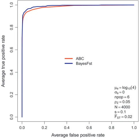
Figure 4.—A comparison of ROC curves for the ABC

method (red) and BayesFst (blue). The curves are based on av-erage true positive and false positive rates measured on 100 sim-ulated data sets. The data are simsim-ulated under the last scenario listed in Table 2 (parameter values are also shown in legend).

Figure 5.—A comparison of ROC curves for the ABC

tested 15 scenarios (Table 2). Each scenario consisted of 100 replicates (i.e., the total number of simulated loci in Table 2 is 150,000). The data sets were analyzed with the ABC algorithm described above and compared with BayesFst. In the ABC analysis 500,000 iterations were used for both the genome-wide parameter estimation

P(ajS(X)) and the locus-specific parameter estimation

P(l_ijU(Xi),S(X)). For the rejection step, we used the 2% nearest points.

An illustration of the application of the method is given in Figures 2 and 3, which are based on one of the data sets generated for the ROC analysis (scenario 15 in Table 2). Figure 2 shows the posterior distribution of genome-wide parameters and Figure 3 shows the posterior probability P(Zi ¼ 1j U(Xi), S(X)) for each locus. In this example it can be seen that the loci that were simulated to be under selection generally have a higher posterior probability to be under selection, and the posterior mode of the number of loci inferred to be under selection,PZi, is close to the true number of 5,

and unsurprisingly rZ has a mode of 0.05. The

demographic parameters are inferred somewhat less well in this example and reflect the influence of the chosen prior. The scaled mutation rate is well estimated, but the inferred value of the scaled migration rate is generally rather too low and weighted toward the prior. The posterior distribution for the variance in mutation rate is broad and tends to follow the prior. The estimated variance among demes in migration rate is rather low and strongly influenced by the prior. The goodness of fit of the model can be examined by seeing how well the symmetric summary statistics S(X) com-puted from the data fit within the prior predictive distribution (see also Ratmann et al. 2009). Since a principal components rotation is used it is relatively straightforward to visualize the fit of the model by plotting the distribution along each axis. An example,

using x–y plots of a selection of axes, is given in

supporting information, Figure S1. Unsurprisingly,

since the data are simulated from the same model used in the analysis, there is a very good fit.

Overall, in the ROC analysis of the 15 scenarios (Table 2), the performance of the ABC method is quite competitive with BayesFst for both s ¼ 0.02 and s ¼

0.1. Although the ABC method often has a slightly lower AUC, the difference is marginal and of the order of the confidence interval. However, in the two scenarios in which there is variability in mutation rate there is superior performance of the ABC method, well beyond the confidence limits of the AUC estimates. Representative numbers, corresponding to rows of Table 2, are given in Figures 4 and 5. The confidence limits are not plotted because they lie close to the estimates. The difference in performance for variable mutation rate arises because the multinomial-Dirichlet model of BayesFst assumes the mutation rate to have a negligible effect on variance in gene frequencies between demes. Thus, when the muta-tion rate is variable, it contributes to addimuta-tional variance in gene frequencies between demes, which in BayesFst is attributed to local selection.

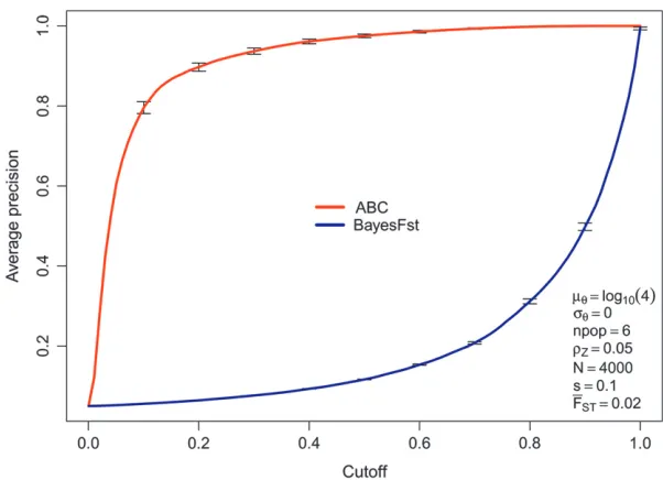
Figure 6 shows that, at least for this scenario for the ABC method, the precision, which is 1 – (false discovery rate), initially increases rapidly with the posterior probability that the locus is under selection (the ‘‘cutoff’’) and then smooths off with a false discovery rate of ,20% after a posterior probability of 0.2. By contrast, the BayesFst classifier shows the inverse behavior—it is most sensitive to change in the classification threshold nearer 1. This difference is not surprising, given the different nature of the methods, but suggests that, with the ABC model, posterior probabilities.0.2 are potentially ‘‘interesting.’’ It should be noted that unlike, for example, Riebleret al. (2008), who used a uniform prior, we have explicitly chosen a prior that gives most weight toP(Zi¼0).

Figure6.—The precision (1false discovery

AN EXAMPLE APPLICATION

We analyzed microsatellite data obtained from a survey of chimpanzee populations from western and central Africa, published by Becquet et al. (2007). These data consist of frequencies sampled in 84 chimpanzees that have been genotyped at 309 micro-satellite loci. The study by Becquetet al. used clustering methods and identified ‘‘western,’’ ‘‘central,’’ and ‘‘east-ern’’ groups. Of these, we used 64 individuals that had precise designations of location (rather than inferred genetically), giving sample sizes, respectively, of 41, 16, and 7. The gene frequencies were then analyzed using BayesFst and our ABC method (Figures 7 and 8).

The goodness of fit of the ABC simulation can be analyzed by comparing the observed summary statistics to the prior predictive distribution (Figure S2). In this case the data are often on the outer edges of the prior predictive distribution in some projections, but are not markedly outlying. The marginal posterior distributions obtained for the hyperparameters (Figure 7) indicate that gene flow is very low, in line with the conclusions of Becquetet al. (2007). This is a scenario in which it is expected that differences in mutation rate among microsatellites will have a major impact on estimates of FST. This is indeed observed: the BayesFst analysis

yields a large number of positives (Figure 8), which, on the basis of the ROC analysis and theoretical expect-ations, are likely to be mainly erroneous. By contrast, the

ABC analysis suggests that there are possibly two in-teresting loci, with posterior probabilities .0.2. This conclusion is based on the results from the simulated data sets above (see Figure 6 and related text for rationale). The estimates of posterior probabilities in the ABC analysis shown in Figure 8 have generally low standard errors (on the logit scale), which indicates a reasonable goodness of fit. If the real data are outliers under the model, then the regression step in ABC is an extrapolation, and estimates tend to have very large standard errors. The microsatellites identified by the ABC analysis are GATA81B01 and ATA28C05. The former has not been mapped inPan troglodytes, but is located on the sixth chromosome in H. sapiens. The

latter has been mapped on the X chromosome of P.

troglodytes and its nearest ORF is LOC739998 of un-known function.

DISCUSSION

The main contribution of this article has been to demonstrate how one can apply ABC-based models to complex scenarios where the number of summary statistics necessarily scales with the number of parame-ters in the model. By treating these cases within the hierarchical Bayesian framework, we show how it is possible to deal with quite complicated problems in a computationally feasible way.

Figure 7.—Marginal

We have introduced two algorithms. Both are based on the idea that two types of summary statistics are computed from the data: symmetric summary statistics

S(X) used to infer the hyperparameters and those that are unit specific, U(Xi), used to infer parameters. Al-though, in our treatment, theS(X) are simple functions of theU(Xi), it should be noted that there is no necessity for consistency in, or any formal relationship between, the summary statistics that are used for inferring the hyperparameters and those for inferring the parame-ters. This distinction is essentially irrelevant providing that the posterior distribution of a is sufficiently accurately approximated. Algorithm 1 is simpler and has the theoretical advantage of sampling from the correct posterior distribution in the limit of zero tol-erance and sufficient statistics. However, it suffers from quite significant problems of storage. This may not be an issue in the longer term as computing resources become more extensive. At the present time, storage is certainly an issue to consider when the number of units (loci, individuals, etc.) is.100. Algorithm 2 avoids this storage problem. However, this algorithm involves an approximation (additional to the use of summary statistics in place of the complete data). In Algorithm 2, the second round of simulation will improve the precision in estimates ofPðlijUðXiÞ;SðXÞÞ ¼

Ð

aPðlijU

ðXiÞ;aÞPðajSðXÞÞda because it samples a from

P(ajS(X)) rather than from P(a). Therefore it may be possible to accept a high proportion of simulated observations, while using a relatively small tolerance. Looking at the problem from the perspective of importance sampling (as in Beaumontet al. 2009; Toni

et al. 2009), it is inviting to consider the weight necessary to correct the error in Algorithm 2. It is straightforward to show that the weight is inversely proportional to

PðXijaÞ ¼ ð

li

PðXijliÞPðlijaÞdli:

That is, if each observationkin step 2 (v) of Algorithm 2 is given a weight that is inversely proportional to the marginal likelihood P(Xi jAk), the resulting weighted sample will be drawn from the correct distribution. Unfortunately the quantity P(Xij a) is not in general easy to compute (otherwise there would be no need to recourse to ABC!). Our main argument in favor of Algorithm 2 is that the approximation will be very slight when the number of units (loci) is large, and scenarios when the number of units is low can be handled by Algorithm 2. The modification, 2a, to Algorithm 2, which is exact, would also be infeasible, requiring separate simulations of step 1 for each locus. Experi-ments (not shown) with toy simulations based on a beta-binomial model suggest that even with 2 units the approximation in Algorithm 2 is good. With the beta-binomial the ABC can be simulated exactly, the weight above can be computed, and Algorithms 1, 2, and 2a can be easily performed and compared.

One potential criticism of the comparison between our ABC approach and that of Beaumontand Balding (2004) is that one uses a model-choice framework and the other is based on BayesianP-values. Thus it might be argued that we have confounded an intrinsic advantage of the model-choice framework with good performance of ABC. However, with low, nonvariable mutation rates there appears to be relatively little difference in perfor-mance of the various approaches to detecting selection that are based on differences in gene frequency. For

example, Beaumontand Balding(2004) showed that

the difference in performance of the moment-based

method of Beaumont and Nichols (1996) was

rela-Figure8.—The posterior probability

tively slight. Riebleret al. (2008), who reformulated the

model of Beaumont and Balding (2004) into an

ex-plicit model-choice framework, demonstrated by means of ROC analysis only a small improvement. Small improvements are also found in Foll and Gaggiotti (2008) and Guoet al. (2009). Therefore we argue that the similar performance of BayesFst and the ABC approach with low, nonvariable mutation rates and the better performance of the ABC method with high and variable mutation rates are not biased by an intrinsic superiority of the model-choice framework.

An additional criticism of our model is that we have not included the ability to detect balancing selection,

which is present in the methods of Beaumont and

Balding (2004), Foll and Gaggiotti (2008), and Riebleret al. (2008). Although it would be straightfor-ward to implement, it was not an aim of this study. It is unlikely that by failing to implement a balancing selection component, we have thereby artificially in-creased the power of the ABC approach in comparison with the multinomial-Dirichlet model. Since the signal of local selection is increased variance in allele frequen-cies among demes, these would not be placed in a balancing selection category anyway. We note that the attempt to use lowFSTas a signal of balancing selection is

logically somewhat problematic. If a locus is truly under balancing selection, it is unlikely that the selection coefficients will be identical in each population. Thus we might typically expect the selection coefficients to vary among populations so the equilibria should vary among populations. For populations with relatively high migration rates it is conceivable that loci under balancing selection may have elevated FST relative to

neutral expectation.

By assuming that the scaled mutation rate u is the same in all demes (while allowing for varying scaled migration rate,Nj), we tacitly assumed constant effective sizeNin each deme. This may be considered somewhat unrealistic, and a future improvement to the model would allow for variation in deme size. This would be preferable to variableubecause then one could include covariance betweenN and u through shared N. Vari-ability in effective size over time could also be consid-ered. Such improvements may reduce the discrepancies observed in the fit of the model to the chimpanzee data

(Figure S2). An advantage of the explicit model-based

approach advocated here is that it is relatively easy to examine model discrepancy (see Ratmann et al. 2009 for detailed discussion).

In addition to the modeling of potential candidates of balancing selection, further improvements to our de-mographic model could include, within the island model framework, the number of demes as a parameter to be inferred. This is potentially important when considering the effects of mutation on gene frequencies. For example, in the case of an infinite-allele, finite-island model with

FSTdefined as in Rousset(1996) we have

FST 1

11ðD=ðD1ÞÞ4Nm14Nm

(for smallmandm). A locus with a higher mutation rate

is therefore expected to have reduced FST but the

strength of the effect depends on the deme size, N. Information about the mutation rate is provided by the metapopulation heterozygosity,HT, which dependsboth

on the deme sizeandon the number of demes because

HT¼ uM

11uM

;

where

uM4DNm 11

1

ðD=ðD1Þ4NmÞ

:

Therefore we expect that very highly heterozygous loci will have reduced FST, potentially leading to false

positives for balancing selection (Beaumont 2008;

Excoffier et al. 2009), but the amount that F_ST is reduced for a given level of heterozygosity depends on the number of demes in the metapopulation. If the number of demes is large, but they have small size, then an elevated mutation rate may have little effect onFST.

Further extensions of the model may include more general migration matrices, and range expansion, to allow for isolation-by-distance effects [necessary to

model human demography (Prugnolle et al. 2005)].

It would also be necessary to consider more general mutation models to allow analysis of sequence data. Much of this could be achieved by the use of

general-purpose packages (Rambaut and Grassly 1997;

Hudson2002; Lavaland Excoffier2004). To demon-strate the utility of the approach we have applied it to the problem of detecting loci under selection. It is impor-tant, however, to emphasize that not all problems can be handled as straightforwardly by a Bayesian hierarchical model, for example, when conditional independence cannot be assumed. There are other areas of application of our ABC method, including population assignment in a more realistic genealogical setting. Its use in fields outside population genetics can also be envisaged.

We are grateful for the constructive critique of two anonymous referees. This work was supported by Biotechnology and Biological Sciences Research Council (BBSRC) grant BBS/B/12776 to M.B. and K.D. and Engineering and Physical Sciences Research Council grant EP/C533550/1 to M.B. E.B. acknowledges grant ANR 07-BDIV-003 (Emerfundis project) for further support. Rothamsted Research receives grant-aided support from the BBSRC.

LITERATURE CITED

Balding, D. J., 2003 Likelihood-based inference for genetic corre-lation coefficients. Theor. Popul. Biol.63:221–230.

Balding, D. J., and R. A. Nichols, 1994 DNA profile match prob-ability calculations: how to allow for population stratification, re-latedness, database selection and single bands. Forensic Sci. Int.

Barton, N., and B. Bengtsson, 1986 The barrier to genetic ex-change between hybridising populations. Heredity56:357–376. Basu, D., 1977 On the elimination of nuisance parameters. J. Am.

Stat. Assoc.72:355–366.

Beaumont_{, M., 2008 Selection and sticklebacks. Mol. Ecol. 17:} 3425–3427.

Beaumont_{, M. A., and D. J. B}alding_{, 2004 Identifying adaptive} ge-netic divergence among populations from genome scans. Mol. Ecol.13:969–980.

Beaumont_{, M. A., and R. A. N}ichols_{, 1996 Evaluating loci for use} in the genetic analysis of population structure. Proc. R. Soc. Lond. Ser. B Biol. Sci.263:1619–1626.

Beaumont, M. A., W. Zhangand D. J. Balding, 2002 Approximate

Bayesian computation in population genetics. Genetics 162:

2025–2035.

Beaumont, M. A., J.-M. Cornuet, J.-M. Marinand C. P. Robert,

2009 Adaptive approximate Bayesian computation. Biometrika

96:983–990.

Becquet, C., and M. Przeworski, 2007 A new approach to estimate parameters of speciation models with application to apes.

Genome Res.17:1505–1519.

Becquet_{, C., N. P}atterson_{, A. C. S}tone_{, M. P}rzeworski_{and D.}

Reich, 2007 Genetic structure of chimpanzee populations.

PLoS Genet.3:10.

Blum_{, M., and O. F}rancxois_{, 2010 Non-linear regression models for} approximate Bayesian computation. Stat. Comput.20:63–73. Cavalli_-Sforza_{, L., 1966 Population structure and human}

evolu-tion. Proc. R. Soc. Lond. Ser. B164:362–379.

Charlesworth, B., M. Nordborg and D. Charlesworth,

1997 The effects of local selection, balanced polymorphism

and background selection on equilibrium patterns of genetic di-versity in subdivided populations. Genet. Res.70:155–174. Crow, J. F., and M. Kimura, 1970 _{An Introduction to Population}

Genet-ics Theory.Harper & Row, New York.

Excoffier_{, L., T. H}ofer_{and M. F}oll_{, 2009 Detecting loci under} selection in a hierarchically structured population. Heredity

103:285–298.

Fagundes, N. J. R., N. Ray, M. Beaumont, S. Neuenschwander, F. M. Salzanoet al., 2007 Statistical evaluation of alternative models of human evolution. Proc. Natl. Acad. Sci. USA104:17614–17619. Fawcett, T., 2006 An introduction to roc analysis. Pattern

Recog-nit. Lett.27:882–891.

Foll, M., and O. Gaggiotti, 2008 A genome-scan method to iden-tify selected loci appropriate for both dominant and codominant markers: a Bayesian perspective. Genetics180:977–993. Gelman, A., 2006 Prior distributions for variance parameters in

hi-erarchical models. Bayesian Anal.1:515–533.

Gemperline, P. (Editor), 2007 Practical Guide to Chemometrics, Ed. 2. Springer, Berlin/Heidelberg, Germany.

Guo, F., D. K. Deyand K. E. Holsinger, 2009 A Bayesian hierarchi-cal model for analysis of single-nucleotide polymorphisms diver-sity in multilocus, multipopulation samples. J. Am. Stat. Assoc.

104:142–154.

Hamilton, G., M. Currat, N. Ray, G. Heckel, M. Beaumontet al., 2005 Bayesian estimation of recent migration rates after a spa-tial expansion. Genetics170:409–417.

Hickerson_{, M. J., and C. P. M}eyer_{, 2008 Testing comparative} phy-logeographic models of marine vicariance and dispersal using a hierarchical Bayesian approach. BMC Evol. Biol.8:322. Hickerson_{, M. J., G. D}olman_{and C. M}oritz_{, 2006 Comparative}

phylogeographic summary statistics for testing simultaneous vi-cariance. Mol. Ecol.15:209–223.

Hudson, R. R., 2002 Generating samples under a Wright-Fisher neutral model of genetic variation. Bioinformatics18:337–338. Joyce_{, P., and P. M}arjoram_{, 2008 Approximately sufficient statistics and} Bayesian computation. Stat. Appl. Genet. Mol. Biol.7:Article 26. Kaplan_{, N. L., R. R. H}udson_{and C. H. L}angley_{, 1989 The}

‘‘hitch-hiking effect’’ revisited. Genetics123:887–899.

Kolmogorov_{, A. N., 1942 Determination of the centre of} disper-sion and degree of accuracy for a limited number of observation. Izv. Akad. Nauk. USSR Ser. Mat.6:3–32.

Laval_{, G., and L. E}xcoffier_{, 2004 Simcoal 2.0: a program to} sim-ulate genomic diversity over large recombining regions in a sub-divided population with a complex history. Bioinformatics20:

2485–2487.

Lewontin, R., and J. Krakauer, 1973 Distribution of gene fre-quency as a test of the theory of the selective neutrality of poly-morphisms. Genetics74:175–195.

Loader, C. R., 1996 Local likelihood density estimation. Ann. Stat. 24:1602–1618.

Marjoram, P., J. Molitor, V. Plagnoland S. Tavare´, 2003 Markov chain Monte Carlo without likelihoods. Proc. Natl. Acad. Sci.

USA100:15324–15328.

McVean, G., and C. C. A. Spencer, 2006 Scanning the human ge-nome for signals of selection. Curr. Opin. Genet. Dev.16:624– 629.

Mevik_{, B. H., and R. W}ehrens_{, 2007 The pls package: principal} com-ponent and partial least squares regression in R. J. Stat. Softw.18:

1–24.

Petry_{, D., 1983 The effect on neutral gene flow of selection at a} linked locus. Theor. Popul. Biol.23:300–313.

Pritchard_{, J. K., M. T. S}eielstad_{, A. P}erez_-Lezaun _{and M. W.} Feldman, 1999 Population growth of human Y chromosomes: a study of Y chromosome microsatellites. Mol. Biol. Evol. 16:

1791–1798.

Prugnolle, F., A. Manicaand F. Balloux, 2005 Geography pre-dicts neutral genetic diversity of human populations. Curr. Biol.

15:R159–R160.

Raiffa, H., and R. Schlaifer, 1961 Applied Statistical Decision Theory. Harvard University Press, Cambridge, MA.

Raiffa, H., and R. Schlaifer, 2000 Applied Statistical Decision Theory. Wiley Classics Library. John Wiley & Sons, New York.

Rambaut, A., and N. Grassly, 1997 Seq-gen: an application for the Monte Carlo simulation of DNA sequence evolution along phy-logenetic trees. Comput. Appl. Biosci.13:235–238.

Rannala, B., and J. A. Hartigan, 1996 Estimating gene flow in is-land populations. Genet. Res.67:147–158.

Ratmann, O., C. Andrieu, C. Wiuf and S. Richardson, 2009 Model criticism based on likelihood-free inference, with an application to protein network evolution. Proc. Natl. Acad. Sci. USA106:10576–10581.

Riebler_{, A., L. H}eld_{and W. S}tephan_{, 2008 Bayesian variable} selec-tion for detecting adaptive genomic differences among popula-tions. Genetics178:1817–1829.

Rousset_{, F., 1996 Equilibrium values of measures of population}

subdivision for stepwise mutation processes. Genetics 142:

1357–1362.

Sabeti, P. C., P. Varilly, B. Fry, J. Lohmueller, E. Hostetteret al.,

2007 Genome-wide detection and characterization of positive

selection in human populations. Nature449:913–918. Sing, T., O. Sander, N. Beerenwinkeland T. Lengauer, 2005 ROCR:

visualizing classifier performance in R. Bioinformatics21:3940– 3941.

Sisson_{, S. A., Y. F}an_{and M. M. T}anaka_{, 2007 Sequential Monte} Carlo without likelihoods. Proc. Natl. Acad. Sci. USA104:1760– 1765.

Slatkin_{, M., 1995 A measure of population subdivision based on} microsatellite allele frequencies. Genetics139:457–462.

Sousa_{, V. C., M. F}ritz_{, M. A. B}eaumont _{and L. C}hikhi_,

2009 Approximate Bayesian computation without summary

sta-tistics: the case of admixture. Genetics181:1507–1519. Spencer_{, C. C. A., and G. C}oop_{, 2004 Selsim: a program to simulate}

population genetic data with natural selection and recombina-tion. Bioinformatics20:3673–3675.

Storz, J. F., and M. A. Beaumont, 2002 Testing for genetic evidence of population expansion and contraction: an empirical analysis of microsatellite DNA variation using a hierarchical Bayesian model. Evolution56:154–166.

Teshima, K. M., G. Coopand M. Przeworski, 2006 How reliable are empirical genomic scans for selective sweeps? Genome Res.

16:702–712.

Toni_{, T., D. W}elch_{, N. S}trelkova_{, A. I}psen _{and M. S}tumpf_,

2009 Approximate Bayesian computation scheme for

parame-ter inference and model selection in dynamical systems. J. R. Soc. Interface6:187–202.

Vitalis, R., K. Dawsonand P. Boursot, 2001 Interpretation of var-iation across marker loci as evidence of selection. Genetics158:

1811–1823.

Wegmann, D., C. Leuenbergerand L. Excoffier, 2009 Efficient approximate Bayesian computation coupled with Markov chain Monte Carlo without likelihood. Genetics182:1207–1218. Weir_{, B. S., and C. C}ockerham_{, 1984 Estimating f-statistics for the}

analysis of population structure. Evolution38:1358–1370. Weir_{, B. S., and W. G. H}ill_{, 2002 Estimating f-statistics. Annu. Rev.}

Genet.36:721–750.

Weir, B. S., L. R. Cardon, A. D. Anderson, D. M. Nielsenand W. G. Hill_{, 2005 Measures of human population structure show}

het-erogeneity among genomic regions. Genome Res. 15: 1468–

1476.

Wright, S., 1931 Evolution in Mendelian populations. Genetics16: 97–159.

Communicating editor: R. Nielsen

APPENDIX: FACTORIZATION OF THE POSTERIOR DENSITY

In thisappendix, we derive the factorization (8), and hence (9), under assumptions that are slightly more general than those set out in (6) and hence (5). In fact we continue to assume that the joint priorP(k, l,a) factorizes as in (6), but we assume that the likelihood functionP(Xjk,l,a) for our model has the factoriza-tion (12). Note that here,ais also a parameter of the model. This formulation covers the special case where the parameterliis simply a function ofkianda.

From the factorization (12) of the likelihood func-tion, and the factorization (6) of the prior density, it follows that the joint density P(a, k, l, X) has the factorization

Pða;k;l;XÞ ¼ Y L

i¼1

PðXijki;li;aÞPðki;lijaÞ

" #

PðaÞ:

ðA1Þ

The marginal densityP(a,X) is therefore

Pða;XÞ ¼ Y L

i¼1

PðXijaÞ " #

PðaÞ; ðA2Þ

where

PðXijaÞ ¼ ð

k ð

l

PðXijki;li;aÞPðki;lijaÞdkdl: ðA3Þ

Dividing (A1) by (A2) we have

Pðk;lja;XÞ ¼Pða;k;l;XÞ Pða;XÞ

¼Y

L

i¼1

PðXijki;li;aÞPðki;lijaÞ PðXijaÞ

¼Y

L

i¼1

Pðki;lija;XiÞ: ðA4Þ

Substituting the right-hand side of (A4) into the factorization

Pða;k;ljXÞ ¼Pðk;lja;XÞPðajXÞ; ðA5Þ

we obtain the factorizations (8) of the posterior density