The Total Branch Length of Sample Genealogies in Populations of Variable Size

DOI: 10.1534/genetics.110.117135

The Total Branch Length of Sample Genealogies in Populations

of Variable Size

A. Eriksson,*

,†

_{B. Mehlig,*}

,1

_{M. Rafajlovic* and S. Sagitov}

‡

*Department of Physics, University of Gothenburg, SE-41296 Gothenburg, Sweden,†Department of Zoology, University of Cambridge, Cambridge CB2 3EJ, United Kingdom and‡Mathematical Sciences, Chalmers University of Technology and

University of Gothenburg, SE-41296 Gothenburg, Sweden Manuscript received March 29, 2010 Accepted for publication June 17, 2010

ABSTRACT

We consider neutral evolution of a large population subject to changes in its population size. For a population with a time-variable carrying capacity we study the distribution of the total branch lengths of its sample genealogies. Within the coalescent approximation we have obtained a general expression— Equation 20—for the moments of this distribution with a given arbitrary dependence of the population size on time. We investigate how the frequency of population-size variations alters the total branch length.

M

ODELS for gene genealogies of biological popula-tions often assume a constant, time-independent population sizeN. This is the case for the Wright–Fisher model (Fisher 1930; Wright 1931), for the Moran model (Moran 1958), and for their representation in terms of the coalescent (Kingman 1982). In real bio-logical populations, by contrast, the population size changes over time. Such fluctuations may be due to catastrophic events (bottlenecks) and subsequent pop-ulation expansions or just reflect the randomness in the factors determining the population dynamics. Many au-thors have argued that genetic variation in a population subject to size fluctuations may nevertheless be described by the Wright–Fisher model, if one replaces the constant population size in this model by an effective population size of the form

Neff ¼ lim L/‘

1 L

XL1 l¼0

1 Nl

!1

; ð1Þ

whereNlstands for the population size in generationl. The harmonic average in Equation 1 is argued to capture the significant effect of catastrophic events on patterns of genetic variation in a population: if, for example, a population went through a recent bottle-neck, a large fraction of individuals in a given sample would originate from few parents. This in turn would lead to significantly reduced genetic variation, param-eterized by a small value ofNeff. (See,e.g., Ewens1982

for a review of different measures of the effective population size and Sjo¨ din et al. 2005 and Wakeley

and Sargsyan 2009 for recent developments of this concept.)

The concept of an effective population size has been frequently used in the literature, implicitly assuming that the distribution of neutral mutations in a large population of fluctuating size is identical to the distri-bution in a Wright–Fisher model with the correspond-ing constant effective population size given by Equation 1. However, recently it was shown that this is true only under certain circumstances (Kaj and Krone 2003;

Nordborg and Krone 2003; Jagers and Sagitov

2004). It is argued by Sjo¨ din et al. (2005) that the concept of an effective population size is appropriate when the timescale of fluctuations ofNlis either much smaller or much larger than the typical time between coalescent events in the sample genealogy. In these limits it can be proved that the distribution of the sample genealogies is exactly given by that of the coalescent with a constant, effective population size.

More importantly, it follows from these results that, in populations with variable size, the coalescent with a constant effective population size is not always a valid approximation for the sample genealogies. Deviations between the predictions of the standard coalescent model and empirical data are frequently observed, and there are a number of different statistical tests quantifying the corresponding discrepancies (see, for example, Tajima1989, Fuand Li1993, and Zenget al. 2006). The analysis of such deviations is of crucial importance in understanding, for example, human genetic history (Garrigan and Hammer 2006). But while there is a substantial amount of work numerically quantifying deviations, often in terms of a single number, little is known about their qualitative origins and their effect upon summary statistics in the popula-tion in quespopula-tion.

1_{Corresponding author:Chalmers University of Technology and} Univer-sity of Gothenburg, SE-41296 Gothenburg, Sweden.

E-mail: [email protected]

The question is thus to understand the effect of population-size fluctuations on the patterns of genetic variation, in particular for the case where the scale of the population-size fluctuations is comparable to the time between coalescent events in the ancestral tree. As is well known, many empirical measures of genetic variation can be computed from the total branch length of the sample genealogy (the expected number of single-nucleotide polymorphisms, for example, is propor-tional to the average total branch length).

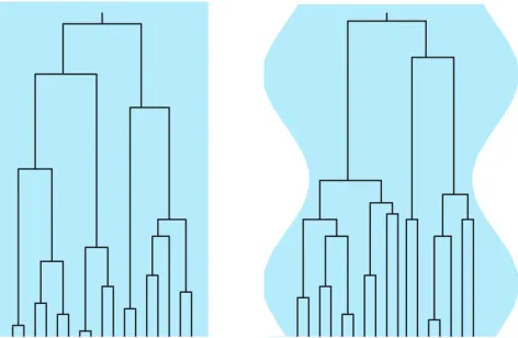
The aim of this article is to analyze the distribution of the scaled total branch lengthTnfor a sample genealogy in a population of fluctuating size, as illustrated in Figure 1. For the genealogy ofn$2 lineages sampled at the present time, the expressionºNTn Ø gives the total branch length in terms of generations. HereºNt Ø is the largest integer#Nt, and the scaling factorNis a suitable measure of the number of genes in the population and serves as a counterpart of the constant generation size of the standard Wright–Fisher model.

A motivating example is given in Figure 2, which shows numerically computed distributionsr(Tn) of the total branch lengths Tn for a particular population model with a time-dependent carrying capacity. The model is described briefly in the Figure 2 legend and in detail in a model for a population with time -dependent carrying capacity. As Figure 2 shows, the

distributions depend in a complex manner on the form of the size changes. We observe that when the frequency of the population-size fluctuations is very small (Figure 2a), the distribution is well described by the standard coalescent result

PðTn#tÞ ¼ ð1et=2Þn1; t$0 ð2Þ

(Hein et al. 2005). When the frequency is very large (Figure 2e), Equation 2 also applies, but with a different time scaling reflecting an effective population size:ton the right-hand side (rhs) in Equation 2 is replaced byt/c withc¼N/Neff. Apart from these special limits, however,

the form of the distributions appears to depend in a com-plicated manner upon the frequency of the population-size variation. The observed behavior is caused by the fact that coalescence proceeds faster for smaller popula-tion sizes and more slowly for larger populapopula-tion sizes, as illustrated in Figure 1. But the question is how to quan-titatively account for the changes shown in Figure 2.

We show in this article that the results of the simulations displayed in Figure 2 are explained by a general expression—Equation 20—for the moments of the distributions shown in Figure 2. Our general result is obtained within the coalescent approximation valid in the limit of large population size. But we find that in most cases, the coalescent approximation works very well down to small population sizes (a few hundred individuals). Our result enables us to understand and quantitatively describe how the distributions shown in

Figure 2 depend upon the frequency of the population-size oscillations. It makes possible to determine, for example, how the variance, skewness, and the kurtosis of these distributions depend upon the frequency of de-mographic fluctuations. This in turn allows us to com-pute the population homozygosity and to characterize genetic variation in populations with size fluctuations.

The remainder of this article is organized as follows. The next section summarizes our analytical results for the moments of the total branch length. Following that, we describe the model employed in the computer simulations. Then, corresponding numerical results are compared to the analytical predictions. And finally, we summarize how population-size fluctuations influence the distribution of total branch lengths and conclude with an outlook.

COALESCENT APPROXIMATION FORMULAS FOR THE MOMENTS Tk

n

For the purpose of coalescent approximation it is convenient to introduce a ‘‘scaled time’’tand a ‘‘scaled population size’’x(t) by writing

Nl¼Nx

lsl

N

[NxðtÞ: ð3Þ

Here N is a suitable counterpart of the constant generation size of the standard Wright–Fisher model assumed to be large. The population is sampled in generationlscorresponding tot¼0, and the timetis

now counted backward in units ofNgenerations, as is common in the coalescent picture. Note that Equation 1 translates into

Figure1.—The effect of population-size oscillations on the

Neff ¼N lim T/‘

1 T

ðT

0

dt xðtÞ

1

: ð4Þ

In this section we show how to calculate the moments Tk

n

for the total (scaled) branch lengthTnfor a given

realization of the curve x(t), making use of results obtained by Tavare´ (1984).

The starting point is the obvious expression for the total time:

Tn¼

Xn

j¼2

jt_j: ð5Þ

Here tjdenotes the time during which the genealogy has jancestral lines. For the population with variable size the timestn,. . .,t2all depend upon the sample size

n; however, this dependence is not made explicit, either here or in the following. As shown by Griffithsand Tavare´ (1994) and Tavare´ (2004), the joint distribu-tion of the times t_j can be written in terms of the variablessj ¼Pn

k¼jtkforj#n(sj¼0 forj.n):

fðt₂;. . .;t_nÞ ¼Y

n

j¼2

bjxðsjÞ1ebj½LðsjÞLðsj11Þ: ð6Þ

Here bj ¼ j(j 1)/2 and LðtÞ ¼Ð₀tdt9xðt9Þ1

is the ‘‘population-size intensity function’’ defined by Griffiths and Tavare´ (1994). In a population of constant size, the variables tjare mutually independent. In general this is not the case: Zivkovic and Wiehe (2008), for example, calculated titj

for a time-varying popu-lation (Equations 2 and 3 in their article), using Equation 6.

Given Equation 5, thekth moment of the distribution ofTnis simply

hTk_ni ¼ X

n21n311nn¼k n2;n3;...;nn

k! n₂!n₃! n_n!n

nn ₂n2_htnn n . . . t

n2

2i;

ð7Þ

where the variablesn_jcan assume values between 0 andk (subject to the constraintn21n31 1nn¼k). In the following we show how the correlation functions of arbitrary order appearing in (7) can be calculated in a very simple manner. Consider first the casek¼1. We have

t_j ¼

ð‘

0

dt1f‘ðtÞ¼jg: ð8Þ

Here‘(t) denotes the number of lines for a particular realization of the coalescent process at timetin a sample of sizen¼‘(0). The indicator function in Equation 8 is unity when‘(t)¼jand zero otherwise. Averaging over realizations gives

ht_ji ¼

ð‘

0

dth1f‘ðtÞ¼jgi ¼

ð‘

0

dt fnjð0;tÞ: ð9Þ

Here fnm(t1, t2) is the conditional probability that n

ancestral lines att1coalesce tomlines at timet2.t1.

Figure2.—Numerically computed distributions rð_T

nÞ of

the scaled total branch lengthsTnin genealogies of samples

of sizen¼10. The model employed in the simulations is out-lined ina model for a population with time-dependent

carrying capacity. It describes a population subject to a

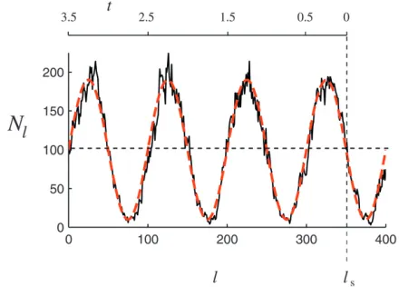
time-varying carrying capacity, Kl ¼ K0(1 1 e sin(2pnl)). The frequency of the time changes is determined byn, and l ¼ 1, 2, 3, . . . labels discrete generations forward in time. The parameterN¼K0describes the typical population size, which is taken here to be equal to the time-averaged carrying capacity. a–e show rðTnÞ for populations with increasingly

rapidly oscillating carrying capacity. The dashed red line in a shows that in the limit of low frequencies the standard co-alescent result, Equation 2, is obtained. The dashed red line in e shows that also in the limit of large frequencies the stan-dard coalescent result is obtained, but now with an effective population size. The dashed red line in d is a two-parameter distribution, Equation 41, derived incomparison between

numerical simulations and coalescent predictions.

Fur-ther numerical and analytical results on the frequency depen-dence of the moments of these distributions are shown in Figure 4. Parameter values used:K0 ¼10,000,e¼ 0.9, and r¼1 (seea model for a population with time-dependent

carrying capacityfor the exact meaning of the intrinsic

growth rater) and (a)nN¼ 0.001, (b)nN¼ 0.1, (c)nN¼

For a constant population size, the coalescent is invariant under time translations,fnm(t1,t2)¼gnm(t2

t1)H(t2t1). HereH(t)¼1 ift.0 and zero otherwise.

The conditional probability gnm(t) was derived by Tavare´ (1984). Form$2 the result is

gnmðtÞ ¼ Xn j¼m

cnmjebjt ð10Þ

cnmj¼ ð1Þjm

2j1

m!ðjmÞ!

Gðm1j1Þ GðmÞ

GðnÞ Gðn1jÞ

Gðn11Þ Gðnj11Þ:

ð11Þ

In the general case of a variable population size, as shown by Griffiths and Tavare´ (1994), the condi-tional probability depends only on the intensityL(t2)

L(t1) during the time interval [t1,t2]:

fnmðt1;t2Þ ¼gnmðLðt2Þ Lðt1ÞÞ: ð12Þ

Now consider the casek¼2. Fori.jwe have simply

titj ¼

ð‘

0

dt11f‘ðt1Þ¼ig

ð‘

0

dt21f‘ðt2Þ¼jg

¼

ð‘

0

dt11f‘ðt1Þ¼ig

ð‘

t1

dt21f‘ðt2Þ¼jg; ð13Þ

because the second indicator function vanishes when t2,t1. Averaging over realizations we find

ht_it_ji ¼

ð‘

0

dt1fnið0;t1Þ

ð‘

t1

dt2fijðt1;t2Þ: ð14Þ

In deriving this result we used the multiplicative rule

h1f‘ðt1Þ¼ig1f‘ðt2Þ¼jgi ¼fnið0;t1Þfijðt1;t2Þ: ð15Þ

Fori¼j, by contrast, we find

t2_j ¼

ð‘

0

dt11f‘ðt1Þ¼jg

ð‘

0

dt21f‘ðt2Þ¼jg

¼2

ð‘

0

dt11f‘ðt1Þ¼jg

ð‘

t1

dt21f‘ðt2Þ¼jg; ð16Þ

which upon averaging yields

ht2 ji ¼2

ð‘

0

dt1fnjð0;t1Þ

ð‘

t1

dt2fjjðt1;t2Þ: ð17Þ

More general correlation functions are readily obtained in terms of multiple integrals over the functions fnm. Inserting into (7) we see that the combinatorial factors (n2!)1 (nn!)1cancel to obtain

hTk_ni ¼k!X

n

m1¼2

Xm1

m2¼2

X

mk1

mk¼2

m1 mk

ð‘

0

dt1fnm1ð0;t1Þ

ð‘

tk1

dtkfmk1mkðtk1;tkÞ:

ð18Þ

Equation 18 provides an explicit expression for the moments of the total branch lengthsTnin populations with population-size variations. The results can be written in a recursive form, particularly convenient for numerical computations,

hTk_nðtÞi ¼kX

n

m¼2

m

ð‘

t

dt9fnmðt;t9ÞhTkm1ðt9Þi; ð19Þ

with initial conditions T0

mðtÞ

¼1 for m $ 2 and

Tk

1ðtÞ

¼0 for k $ 1. Here Tn(t) is the total time corresponding to the genealogy ofnsequences sampled at timetin the past given a population-size curvex(t). Note thatt¼0 corresponds to the present time, so that Tn(0)[ Tn. In a population of constant size, Tn(t) is independent oft.

Equation 18 or 19 expresses thekth moment ofTnin terms of a 2k-fold sum [according to (10) each factor of fnimi contains a sum overji]. Equation 18 can be further

simplified by explicitly performing the sums over m1,. . .,mk. This results in

hTkni ¼k!

Xn

j1¼2

X

jk1

jk¼2 dn;j1;...;jk

ð‘

0

dt1ebj1Lðt1Þ ð‘

t1

dt2ebj2½Lðt2ÞLðt1Þ

ð‘

tk1

dtkebjk½LðtkÞLðtk1Þ: ð20Þ

The coefficients are determined by recursion:

dn;j¼ Xj m¼2

m cnmj¼ ð2j1Þð11ð1ÞjÞ

2n1

nj

2n1

n

;

ð21Þ

dn;j1;...;jk ¼

Xj1

m¼j2

m cnmj1dm;j2;...;jk: ð22Þ

For the particular casek¼1 our result corresponds to an expression derived by Austerlitz et al. (1997) and

Slatkin (1996) and also to the result obtained by

summing Equation 1 in Zivkovic and Wiehe(2008). Fork¼2, the coefficientsdn;;j1;j2are tabulated in Figure A1 in theappendixfor small values ofn. In general, the nested integrals in Equation 20 cannot be simplified further; their form expresses the correlations of the timest_jdue to population-size variations.

hTk 2i ¼k!2k

ð‘

0

dt1f22ð0;t1Þ ð‘

t1

dt2f22ðt1;t2Þ ð‘

tk1

dtkf22ðtk1;tkÞ ¼k!2k

ð‘

0

dt1 ð‘

t1 dt2

ð‘

tk1

dtkf22ð0;tkÞ ¼2kk ð‘

0

dt tk1eLðtÞ:

ð23Þ This representation demonstrates how the expression (18) simplifies whenk.n.

We conclude this section by briefly describing three different scenarios where our main result (Equation 18) is applicable. First, Sjo¨ din et al. (2005) discussed a model where the scaled population sizex(t) defined by Equation 3 may assume two values, 1 andx. The pop-ulation size randomly jumps from 1 toxat ratel and back at ratelx. Initially the population size isx(0)¼1. Our result (Equation 18) is directly applicable to a given realization of the random processx(t). We denote the ensemble average over realizations of x(t) byhTk

ni. By averaging Equation 18 over the corresponding distribu-tion ofLwe find

hTni ¼

Xn

j¼1

dn;j

l1l_x1bj=x

bjðl=x1lx1bj=xÞ

: ð24Þ

Higher moments can be obtained in a similar fashion. This provides explicit expressions for the fluctuations of Tnin the case of slow, fast, and intermediate population-size changes. This model is particularly suited to examine the limit of fast population-size fluctuations l¼l_x/‘. As expected, the standard Kingman co-alescent, Equation 2, is recovered but now with an effective population sizeNeff¼N/cwithc¼(11x1)/2.

Second, intermediate population-size variations over many generations give rise to deviations from the standard Kingman behavior. The deviations are ex-pected to be most significant when the timescale of the size variations is comparable to the times between coalescent events. Such intermediate population-size variations are commonly interpreted as due to a changing environment. In this case it is inappropriate to average over an ensemble of random population size curvesx(t). The task is instead to describe the fluctua-tions of Tn conditional on a particular, externally imposed form of x(t). An example is the question: How does a recent bottleneck influence the distribution of Tn? To compute the kth moment of Tn, a k-fold integration is required. In general this must be per-formed numerically. However, in the case of piecewise constant functions x(t) the multiple integrals are straightforward to evaluate. If, on the other hand, the function x(t) is sufficiently ‘‘smooth,’’ the multiple integrals can be evaluated in closed form in the limits of slowly and rapidly varying population sizes as dem-onstrated below.

Third, in general stochastic population dynamics subject to a slowly changing environment may exhibit both slow changes due to an externally imposed change of the environment (in the form of a time-changing

carrying capacity, for example) and ‘‘fast’’ (generation-to-generation) changes due to the random population dynamics. In the next two sections such a model is introduced and analyzed by means of Equation 18. The analysis is simplified by the observation that the fast size variations are irrelevant when their amplitude remains small. In this case Equation 18 may be evaluated using a deterministic population-size curve that is averaged over the fast changes. In the model discussed in the next two sections this curve is given by the deterministic time dependence of the carrying capacity.

A MODEL FOR A POPULATION WITH TIME-DEPENDENT CARRYING CAPACITY

The purpose of this section is to describe a modified Wright–Fisher model with a fluctuating carrying capac-ity. This model is used in the numerical simulations of sample genealogies described in the next section. Recall the three key assumptions of the Wright–Fisher model: (a) constant population size, (b) discrete, nonoverlap-ping generations, and (c) a symmetric multinomial distribution of family sizes. We have adopted the fol-lowing approach: in our simulations, assumptions b and c are still satisfied, but assumption a is relaxed.

We study a large but finite population of fluctuating size Nl, where l ¼ 1, 2,. . . labels the discrete, non-overlapping generations forward in time. The model we have adopted is the following: consider a generationl consisting ofNlindividuals. The number of individuals in generationl11 is then given by

Nl11¼

XNl

j¼1

jj; ð25Þ

where the random family sizesjjare independent and identically distributed random variables having a Pois-son distribution with parameter ll (specified below). Consequently the number Nl11 is Poisson distributed

with meanNll_l.

This model exhibits a fluctuating population sizeNl, rapidly changing from generation to generation. As pointed out in the Introduction, in large populations such fluctuations are averaged over by the ancestral coalescent process and can be captured in terms of an effective population size. The resulting genealogies are simply described by Kingman’s coalescent for a constant effective population size of the form (1) or (4).

l_l¼ 11r 11rNl=Kl11

ð26Þ

for a certain parameter valuer . 0. Here Kl11is the

carrying capacity in generation l 1 1. If the environ-mental changes affected the population through fertil-ity variations,Kl11would be replaced byKlin Equation

26. Equation 26 is chosen so that the population ceases to grow on average when the carrying capacity is reached (l_l¼1 for Nl ¼Kl11). When the population

size is small andr>1, the population growth follows the logistic law, ll ¼ 1 1 r(1 Nl/Kl11), where r is the

intrinsic growth rate. The particular form of Equation 26 ensures thatll.0.

Note that fluctuations ofNlin this model are due to two different sources: rapid fluctuations are caused by the randomness of the family sizes, and slow fluctuations are caused by the time dependence of the carrying capacity. Our choice for the time dependence ofKl is dictated by the following considerations. The aim is to describe the influence of a fluctuating population size upon the statistics of genetic variation. To this end we need to consider the functional form of Kl. A simple choice forKlis a periodically varying function, such as

Kl ¼K0½11esinð2pnlÞ;e2 ð0;1Þ;n2 ð0;‘Þ: ð27Þ

Note that a more complex dependence ofKluponlcan be obtained from superpositions of such functions with different amplitudeseand frequenciesn. Here we use simply (27) and investigate how the statistics of genetic variation in a sample depend upon frequency of the fluctuations inKl.

Figure 3 shows a realization of a curveNlobtained in this manner (the choice of parameters is given in the Figure 3 legend). Figure 3 clearly exhibits fluctuations in Nl on two timescales, fast and slow. As explained above, the fast fluctuations are irrelevant provided their amplitude is sufficiently small. In this case we expect that the distribution of Tn can be described by a population-size curve that is averaged over the fast fluctuations. In the present model, averaging over the fast fluctuations results in a deterministic population-size curve determined by the carrying capacity (27). This curve is shown in Figure 3 as a dashed line.

Note that conditional on the sequence of population sizes, the genealogy of a set of individuals sampled in generationlcan be determined recursively by randomly choosing ancestors in the preceding generations. This is ensured by the assumption that, conditioned on the values ofNlandNl11, the family sizes follow a symmetric

multinomial distribution MnðNl11;1=Nl; . . . ;1=NlÞ. The resulting correspondence with the Wright–Fisher rule of reproduction ensures that the genealogies can be determined recursively in the way suggested above.

In the next section we analyze results of three sets of 10,000 computer simulations for this population model

with parametersr ¼1 ande¼0.9 and for a range of values for n. The three sets differ in the values for the average carrying capacity that are chosen to beK0¼100,

K0¼1000, andK0¼10,000. The population is sampled

in generationls(see Figure 3), which is chosen so that

2nlsbecomes an odd natural number. This implies that

Kls¼K0 and that the population size was declining towardKls in the most recent past.

COMPARISON BETWEEN NUMERICAL SIMULATIONS AND COALESCENT PREDICTIONS

In this section we discuss the numerically computed distributions shown in Figure 2 in terms of Equation 18. The shapes observed in Figure 2 are conveniently characterized in terms of their mean hTni, variance, skewness, and kurtosis:

varðTnÞ ¼ hT2ni hTni2;

skewðTnÞ ¼

hðTn hTniÞ3i

var3=2ðTnÞ

; ð28Þ

kurtðTnÞ ¼

hðTn hTniÞ4i

var2ðTnÞ

: ð29Þ

Recall that for a normal distribution the skewness van-ishes, and the kurtosis equals three. We can write the skewness and kurtosis in terms of the moments Tk

n

using

ðTnhTniÞ3

¼ T3n

3T2n

Tn

h i12hTni3and ðTnhTniÞ4

¼ T4 n

4T3 n

Tn h i16T2

n

Tn h i2_3T

n h i4_:

The moments Tk

n

are evaluated by means of Equations 18 and 19 as functionals of the scaled

Figure3.—One realization of the curve_N

lobtained from

simulations of the model described ina model for a

popu-lation with time-dependent carrying capacity (black

population size x(t) followed backward in time. With stochastically fluctuating sizes the scaled population size x(t) also becomes a random process. As Figure 3 in-dicates, the random fluctuations around the determin-istic carrying capacity function are relatively small and we expect that such generation-to-generation fluctua-tions are irrelevant for the distribution of Tn. We therefore disregard the fast (random) fluctuations of the population sizes and define functionx(t) determin-istically by

xðtÞ ¼11esinðvtÞ: ð30Þ

This is obtained from an analog of Equation 3 when the population is sampled in generationls(as indicated in

Figure 3):

Kl ¼Nx

lsl

N

: ð31Þ

Here (27) was used withv¼2pnN, and N¼K0. Note

that the particular form (30) ofx(t) depends upon when the population is sampled. Had the population been sampled at a different time, a different curvex(t) could have resulted, leading in turn to a different distribution r(Tn) ofTn, since the distribution depends, for exam-ple, upon whether most recently the population was expanding or declining.

Our results are summarized in Figure 4. It shows how the mean, variance, skewness, and kurtosis of the distribution of Tn depend on the scaled frequency v of the population size variation, Equation 30. Shown are results of numerical simulations of the model described in the previous section (symbols) and results obtained within the coalescent approximation using Equation 19. We observe that the coalescent approximation describes the results of the numerical simulations well, even for small population sizes.

In the numerical simulations we have found that, for very small population sizes, random fluctuations ofNl around the time-dependent carrying capacity Kl be-come increasingly important. Since we suspected that the small deviations observed in Figure 4a forK0¼100

were due to such fluctuations, we performed slightly modified simulations imposing a deterministic law uponNlby forcingNl¼Klin every generation [where Klis given by (27)]. Comparison of the corresponding results (not shown) with Figure 4a indicates that the deviations forK0¼100 at large frequencies are indeed

caused by the stochastic fluctuations in the population dynamics underlying Figure 4a. A different interpreta-tion of this effect is the following: when the populainterpreta-tion size is very small, and when e is close to unity, the population may exhibit a nonnegligible probability of becoming extinct during the expected time to the most recent common ancestor for a sample of sizen. In this

case we have conditioned on the existence of the population during 100K0 generations using rejection

sampling. In practice this avoids extinction, but it leads to a biased size distribution.

Consider now the frequency dependence of the moments shown in Figure 4. It can be qualitatively and quantitatively understood using Equation 20 together with the following expression forL(t):

LðtÞ ¼ ðt

0 ds

11esinðvsÞ

¼Øvt=2p11=2ø ð1=pÞarctanðe= ffiffiffiffiffiffiffiffiffiffiffiffiffi

1e2 p

Þ1ð1=pÞarctanððtanðvt=2Þ1eÞ=pffiffiffiffiffiffiffiffiffiffiffiffiffi1e2_Þ

ðv=2pÞpffiffiffiffiffiffiffiffiffiffiffi1e2 :

ð32Þ

Here Øzøis the smallest integer larger than z. Next we discuss the asymptotical formulas for small and large frequenciesv.

In the limit of v/0, Equation 32 simplifies to LðtÞ t 1

2evt

2_{. Inserting this into (20) we find}

approximately

hTni ¼2hn14ðgnhn=nÞev1oðvÞ; v/0: ð33Þ

Herehn¼Pn1

j¼1 j

1_{andgn ¼}Pn1

j¼1 j

2_{. Equation 33 is}

shown in Figure 4a as a dashed-dotted line. For the variance we find the approximate expression

varðTnÞ ¼4gn116 fngn1 hngn

n

ev1oðvÞ; v/0;

ð34Þ

withfn ¼Pnm¼11ðm

3_1m2_hm

11Þ. The limiting value for

zero frequency is that of the standard coalescent with constant population size. Equation 34 is shown in Figure 4b as a dashed-dotted line. Similarly the standard results for the constant-size coalescent are obtained for the skewness and for the kurtosis in the limit ofv/0. This limiting behavior is illustrated in Figure 2a, which shows that the distribution of Tn approaches that for King-man’s coalescent for a constant population size in the limit of small frequencies. We note that for v>1, the population-size dependence is essentially that of a declining population, because the time to the most recent common ancestor is reached before the first maximum inx(t) going backward in time (see Figure 3 and Equation 30).

LðtÞ ¼ ffiffiffiffiffiffiffiffiffiffiffiffiffit 1e2

p arctanðe=

ffiffiffiffiffiffiffiffiffiffiffiffiffi 1e2 p

Þ vpffiffiffiffiffiffiffiffiffiffiffiffiffi1e2 1oðv

1_{Þ; v/‘: ð35Þ}

For large frequencies, the functionL(t) is well approx-imated by a shifted linear function

LðtÞ tc1L0: ð36Þ

Herecdetermines the effective population size accord-ing to Equation 4:Neff¼N/cwith

c ¼ lim

T/‘ 1 T

ðT

0

dt

11esinðvtÞ ¼ 1

ffiffiffiffiffiffiffiffiffiffiffiffiffi

1e2

p : ð37Þ

The parameter c describes the influence of the de-mographic fluctuations upon the part of the genealogy in the distant past. The small offset

L0¼

arctane=pffiffiffiffiffiffiffiffiffiffiffiffiffi1e2_c

v

ec

v forenot too close to unity ð38Þ

describes the influence of demographic changes on the most recent part of the genealogy. Inserting the approx-imation (36) into (20) we find for large frequencies (and when the amplitudeeis not too close to unity)

hTni ¼2hnc11nev11oðv1Þ; v/‘: ð39Þ

The first term in (39) is the expected time of Kingman’s coalescent for a constant effective population sizeNeff¼

N/c. The curve corresponding to (39) is shown as a dashed line in Figure 4a. We infer that corrections to the standard coalescent result are significant when the sample size is large, the amplitude of the size oscil-lations is not too small, and the frequencyvis of order

unity. This is consistent with the results of Sjo¨ dinet al. (2005).

We now discuss the behavior of the variance shown in Figure 4b. For the second moment we find

hT2_ni 4c2ðgn1h2nÞ1

4nhne

vc : ð40Þ

The first term in Equation 40 corresponds to the second moment ofTnin Kingman’s coalescent with a constant effective population size. The second term in (40) represents a correction due to finite but large frequen-cies; it depends in a simple fashion on the effective population-size parametercand on the sample sizen.

Comparing Equations 39 and 40, we arrive at the conclusion that the corresponding correction for the variance var(Tn) vanishes. This is consistent with the fact that, at large frequencies, the variance ofTnis surpris-ingly insensitive to changes in frequency (as opposed to the behavior ofhTni, see Figure 4, a and b). In fact, the limiting value (shown in Figure 4b as a dashed line) is a very good approximation to var(Tn) down tov3.

Consider now the skewness and the kurtosis shown in Figure 4, c and d. Their behavior is similar to that of the variance: forv. 3, the skewness and the kurtosis are essentially independent of v. The results shown in Figure 4 imply that over a large range of frequencies, the distribution of the total branch lengthsTncan be approximated as follows: the distribution is essentially that of the standard Kingman coalescent with an effective population size, but the distribution is shifted such that its mean is given by Equation 39, rather than by 2hn/c.

Figure 4.—Mean (a),

variance (b), skewness (c), and kurtosis (d) of the dis-tribution ofTnfor samples

of size n ¼ 10, as a func-tion of the frequency of the population-size fluctua-tions. Shown are results of numerical simulations (10,000 simulations with N¼K0,K0¼100, triangles; K0¼ 1000, diamonds; and K0 ¼ 10,000, circles) as well as results computed within the coalescent ap-proximation described in

coalescent

approxima-tion formulas for the

moments(red solid lines).

One may wonder when this ‘‘rigid shift’’ occurs. Given Equation 18 it is straightforward to work out the fluctuations of the times tj within the approximation (36). We find that forj,n, the expected value oftjis exactly that of the standard Kingman coalescent with effective population size. But forj¼nit is rigidly shifted by L0/c. This indicates that the genealogies are

essentially those of the standard coalescent, but modi-fied by an initial rigid shift. In the parameter regime discussed here, the distribution of times is expected to be well approximated by a two-parameter family of distributions,

PðTn,zÞ 1exp

zc1nL₀ 2

n1

ð41Þ

whenzc.nL0, andP(Tn,z)0 for smaller values of

z. The first parameter determines the effective popula-tion size. It parameterizes the slope of the funcpopula-tionL(t) at large times and describes the demographic effect on the distant past of the genealogy. The second parameter, L0describes the influence of the demographic

fluctua-tions on the initial part of the sample genealogy. This parameter can be negative (recent population decline, this is the case shown in Figure 3) or positive (recent population expansion). WhenL0.0, the distribution

r(Tn) is rigidly shifted to the left. In this case the approximation (36) is expected to break down when the body of the distribution reachesTn¼0.

Note that the distribution (41) cannot be described by a single parameter (a ‘‘generalized effective popula-tion size’’). The approximapopula-tion (41) was used to gen-erate the red dashed curve in Figure 2d.

CONCLUSIONS

The aim of this article was to investigate how the frequency of population-size fluctuations determines the shape of the distribution of total branch lengths of sample genealogies and thus of statistical measures of genetic variation.

We performed simulations for a modified Wright– Fisher model of a population subject to a time-periodically varying carrying capacity and determined the distribution of the total branch lengths, shown in Figure 2. We characterized how the shapes of the distributions depend upon the frequency of the pop-ulation-size fluctuations by computing the frequency dependence of the moments of these distributions. We could explain these dependencies in terms of coales-cent approximations. In particular, we derived a general

expression—Equation 20—for the moments Tk

n

in populations subject to smooth population changes of otherwise arbitrary form.

Our results show how quickly (or slowly) the standard coalescent result for a constant (effective) population sizes is recovered in the limits of large and small

frequencies. More importantly, our coalescent results allow us to determine how significant deviations are at large but finite frequencies. In this case we argued that at large frequencies, the distribution ofTnis essentially that of the standard Kingman coalescent with an effective population sizeNeff¼N/c, but with a shifted mean value

hTni

2 c

Xn1 j¼1

1 j 1

ne

v forv?1: ð42Þ

The first term on the rhs corresponds to the result of the standard Kingman coalescent with a constant effective population size. The second term on the rhs is the correction term resulting from the population-size variations (e is the amplitude of the population-size oscillations,vis its frequency, andnis the sample size). We infer that corrections to the standard coalescent result are largest when the sample size is large and the amplitude e of the size fluctuations is not very small. This is consistent with the results of Sjo¨ dinet al.(2005). Last but not least we found that the coalescent approximation yields a reliable description of the numerical data, even for very small populations.

We close with a number of remarks. First, Equation 20 is easily generalized to describe the moments of observ-ables that are polynomial functions of the times t_j. Particularly simple is the case of observablesAthat are linear functions of the timest_j,An¼Pn

j¼2ajtj. In this case thekth moment ofAnis given by Equation 20, but with modified coefficients: the factorsmin Equations 21 and 22 are replaced byam.

Second, some observables [such as theF-statistic (Fu and Li1993)] can be written as linear functions oft_j, but with random coefficients. In this case too it is possible to explicitly compute the moments of the distribution of the observable. These two questions are addressed in a separate article (S. Sagitov, M. Rafajlovic, B. Mehlig, and A. Eriksson, unpublished results).

Third, Equation 19 allows us to determine in a transparent fashion how the fluctuations ofTndepend upon the time at which the population is sampled. This will make it possible to discuss, for example, how Tajima’s D-statistic or theF-statistic depends upon the time of sampling after a bottleneck, a population expansion, or a decline.

expect to observe strong correlations betweentiandtj and thus deviations from the standard Kingman co-alescent. Second, for small values ofiandjwe expect the times ti and tj to decorrelate and to follow the distribution of the standard coalescent (with an effec-tive population size).

Fifth, the model introduced in a model for a

population with time-dependent carrying capacity

assumes a carrying capacity that varies sinusoidally, with a single frequency. It turns out, however, that our findings (summarized in Equation 41) are valid for arbitrary time-dependent fluctuations with a sufficiently strong and narrow mode at high frequencies. Examples are linear combinations of high-frequency oscillations or stochastic fluctuations around a constant population size, with a sufficiently narrow frequency spectrum. In this case, too, we expect thatL(t) is well approximated by (36). If this is the case, the distribution of times is of the form (41) whenL0is small.

Taken together, the results derived in this article give a rather complete understanding of the fluctuations of empirical observables due to population size variations. These results will be significant when attempting to disentangle the effects of population-size variations from other factors influencing genetic variation.

Our results raise the question under which circum-stances the deviations from standard coalescent behav-iors due to population-size fluctuations (Figures 2 and 4) are most likely to strongly affect the interpretation of empirical data. As our analysis indicates, the deviations become substantial when the frequencyv¼2pnNis of order unity. Heren is the frequency of the population size variations, Equation 30, andNis a suitable measure of the population size. In other words, rapid population-size fluctuations will have the strongest effect (other than simply determining the effective population size) in small local subpopulations with restricted gene flow between subpopulations with different fluctuations. The deviations are expected to be smaller at larger spatial scales, because the ancestral process averages over the spatial fluctuations. More generally, we con-clude that deviations from standard coalescent behavior are expected for populations subject to an environment that changes as a function of space and time on neither too small nor too large length and timescales. An example for such a population is the marine snail Littorina saxatilis. Its habitat on the Northern coast of Bohusla¨n (Sweden) is fragmented into subpopulations with strongly restricted gene flow between them, and effective population sizes of subpopulations have been found to be very small (K. Johannesson, personal

communication). Starting from the results derived in this article, we hope to determine gene genealogies in such fragmented populations subject to variations of population size in space and time.

We thank two anonymous reviewers for helpful comments and suggestions. Support from Vetenskapsra˚det, The Bank of Sweden Tercentenary Foundation, and the Centre for Theoretical Biology at the University of Gothenburg is gratefully acknowledged.

LITERATURE CITED

Austerlitz_{, B., B. J}ung_-Muller_{, B. G}odelle _{and P. G}ouyon_, 1997 Evolution of coalescence times, genetic diversity and structure during colonization. Theor. Popul. Biol.51:148–164. Ewens, W., 1982 The concept of the effective population size.

Theor. Popul. Biol.21:373–378.

Fisher_{, R. A., 1930 The Genetical Theory of Natural Selection.} Claren-don Press, Oxford.

Fu_{, Y., and W. L}i_{, 1993 Statistical tests of neutrality of mutations.} Genetics133:693–709.

Garrigan_{, D., and M. F. H}ammer_{, 2006 Reconstructing human} origins in the genomic era. Nat. Rev. Genet.7:669–680. Griffiths_{, R., and S. T}avare´_{, 1994 Sampling theory for neutral}

al-leles in a varying environment. Philos. Trans. R. Soc. Lond. B344:403–410.

Hein, J., M. H. Schierupand C. Wiuf, 2005 Gene Genealogies,

Varia-tion and EvoluVaria-tion: A Primer in Coalescent Theory.Oxford University Press, London/New York/Oxford.

Jagers, P., and S. Sagitov, 2004 Convergence to the coalescent in populations of substantially varying size. J. Appl. Probab.41:368– 378.

Kaj_{, I., and S. K}rone_{, 2003 The coalescent process in a population} with stochastically varying size. J. Appl. Probab.40:33–48. Kingman_{, J., 1982 The coalescent. Stoch. Proc. Appl.13:235–248.} Moran, P., 1958 Random processes in genetics. Proc. Camb. Philos.

Soc.54:60–71.

Nordborg_{, M., and S. K}rone_{, 2003 Modern Developments in}

Popula-tion Genetics: The Legacy of Gustave Male´cot, pp. 194–232. Oxford University Press, Oxford.

Sjo¨ din, P., I. Kaj, S. Krone, M. Lascoux and M. Nordborg, 2005 On the meaning and existence of an effective population size. Genetics169:1061–1070.

Slatkin_{, M., 1996 Gene genealogies within mutant allelic classes.} Genetics143:579–587.

Tajima, F., 1989 Statistical method for testing the neutral mutation hypothesis by DNA polymorphism. Genetics123:585–595. Tavare´, S., 1984 Lines of descent and genealogical processes, and

their application in population genetics models. Theor. Popul. Biol.26:119–164.

Tavare´_{, S., 2004 Ancestral Inference in Population Genetics, pp. 1–188.} Springer, Berlin.

Wakeley_{, J., and O. S}argsyan_{, 2009 Extensions of the coalescent} effective population size. Genetics181:341–345.

Wright_{, S., 1931 Evolution in Mendelian populations. Genetics16:} 97–159.

Zeng, K., Y. Fu, S. Shiand C. Wu, 2006 Statistical tests for detecting positive selection by utilizing high-frequency variants. Genetics

174:1431–1439.

Zivkovic_{, D., and T. W}iehe_{, 2008 Second-order moments of} segre-gating sites under variable population size. Genetics180:341– 357.

APPENDIX: COEFFICIENTSdn;j1;j2FOR n¼2,. . ., 10

In Figure A1 we give the coefficientsdn;j1;j2determining the second moment T 2

n

according to Equation 20 for

n¼2,. . ., 10. Note that the coefficient forn¼2 is consistent with Equation 23.

FigureA1.—Coefficients_d

n;j1;j2 occurring in Equation 20