ABSTRACT
SPRENG, RACHEL LYNN. Methods for the Reuse of Public Data in Gene Expression Studies. (Under the direction of Dahlia Nielsen).
The collection of data held in genomics repositories such as the Gene Expression Omnibus (GEO) contains a wealth of information about gene expression on a large scale. Comparing gene expression across multiple studies could provide more power to answer questions of interest than analyzing a single study alone. Here, we have compiled a set of human microarray studies taken from GEO and we propose several gene expression analysis methods incorporating this data.
Next, we used external data to identify genes associated with a given phenotype, even in the absence of a control group in the study of interest. We collected a baseline distribution of gene expression measurements from the control groups of 33 independent studies, comparing the population of interest to this reference control group rather than the controls from the same study. A gene was identified as significant if the p-value from a t-test was below the desired threshold and the mean expression in the treatment group of interest was in the upper or lower tail of the reference distribution. To validate the selected genes, we determined whether the selected subset of genes sufficiently clustered data into known groups. Though this is not confirmation of association, it does indicate that the set of genes selected is enriched for genes that are differentially expressed between the phenotype of interest and controls. Additionally, this approach was applied to several independent studies representing the same phenotype to determine similarity of results.
Finally, we used the data collected from GEO to examine correlation of expression profiles for pairs of genes in different phenotypic populations. For 450 selected pairs of genes, we compared the correlation of expression profiles across 64 studies, subset by phenotype into 96 disease groups and 42 control groups. We evaluated whether correlation was relatively consistent within control groups and if median correlation was significantly different from zero. We then identified phenotypes for which correlation changed, defining a disease group as an outlier if the correlation of expression values within that group was in the lower 5% of control group correlations if correlation on average was positive or upper 5% of control group correlations if correlation on average was negative.
Methods for the Reuse of Public Data in Gene Expression Studies
by
Rachel Lynn Spreng
A dissertation submitted to the Graduate Faculty of North Carolina State University
in partial fulfillment of the requirements for the degree of
Doctor of Philosophy
Bioinformatics
Raleigh, North Carolina 2017
APPROVED BY:
_______________________________ ______________________________
Dahlia Nielsen Jeffrey Thorne
Committee Chair
________________________________ ________________________________
ii Dedication
iii Biography
iv Acknowledgments
This work was made possible by a training grant from the National Institute of Environmental Health Sciences (T32ES007329).
I would like to thank my advisor, Dr. Dahlia Nielsen, for giving me the opportunity to work with her and for her guidance, patience, and support. I thank Dr. Rob Smart (and his students) for allowing me to attend and present at lab meetings, for patiently teaching me about biological research, and for valuable feedback. I thank my additional committee members, Dr. Jeff Thorne and Dr. David Reif, for their time and contributions. Thank you to Dr. Colleen Doherty for valuable discussions and suggestions.
To the BRC faculty, staff, students, post-docs, and alumni, thank you for all of your help and encouragement, and for making the BRC such a friendly environment.
To my professors and classmates at Rowan, thank you for preparing me for my time at NC State. A very special thank you to Dr. Karen Magee-Sauer. You had such faith in me, and without your encouragement and guidance, I don’t think I would have ended up in graduate school.
Finally, I’d like to thank my church community, my friends, and my family. Without your
v Table of Contents
List of Tables ... vi
List of Figures ... vii
Chapter 1 Introduction and Background ... 1
1.1Introduction ... 1
1.2Prior Results in Data Integration ... 1
1.3A Novel Approach to Integrate Public Gene Expression Data ... 3
1.3.1 Variance of Gene Expression ... 3
1.3.2 Mean of Gene Expression ... 4
1.3.3 Correlation of Gene Expression ... 5
1.3.4 Conclusions... 5
References ... 6
Chapter 2 Comparing variance in gene expression across a collection of public studies to reduce data dimensionality prior to clustering ... 8
2.1 Abstract ... 8
2.2 Introduction ... 9
2.3 Results and Discussion... 12
2.3.1 Biological Studies ... 13
2.3.2 Simulated Data ... 18
2.4 Conclusions... 20
vi
References ... 35
Chapter 3 Comparing mean gene expression across a collection of public studies to identify differentially expressed genes ... 37
3.1Abstract ... 37
3.2Introduction ... 38
3.3Results and Discussion... 40
3.3.1 Accuracy of Clustering on Identified Genes ... 41
3.3.2 Comparing Results from Multiple Lung Cancer Studies ... 43
3.4Conclusions... 43
3.5Method Details ... 45
References ... 50
Chapter 4 Comparing correlation of gene expression across a collection of public studies ... 54
4.1Abstract ... 54
4.2Introduction ... 54
4.3Results and Discussion ... 56
4.4Conclusions ... 60
4.5Method Details ... 60
References ... 67
Chapter 5 Discussion and Concluding Remarks... 68
5.1Summary of Results ... 68
vii
Appendices ... 71
Appendix A ... 72
Appendix B ... 74
Appendix C ... 75
viii List of Tables
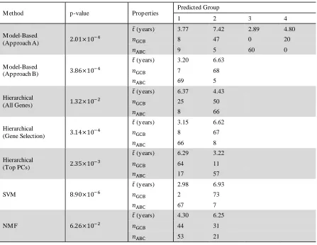
Table 2.1 Summary of Diffuse Large B-Cell Lymphoma (DLBCL) Results. Summary of group sizes (subset by group label as defined by Alizadeh et al.), mean survival time, 𝑡̅ (in years), and p-value for the test of difference in survival of the groups resulting from each method. For reference, Alizadeh et al.’s groups have a p-value of 4.69×10⁻⁵, with the
GCB-DLBCL group having a mean survival time of 6.78 years and the ABC-DLBCL group having a mean survival time of 3.09 years. Group labels by the various methods are arbitrary, thus group 1 resulting from one method does not necessarily correspond to group 1 resulting from any
other method. ... 31 Table 2.2 Summary of Results on Biological Studies. Summary of the results of
various methods on 10 biological datasets (labeled by their GEO accession number). Shown are the calculated values of the Jaccard Similarity Coefficient, 𝐽, a measure of concordance between known groups and the groups predicted by different methods. For the clustering methods applied to randomly selected genes, 𝐽 is a mean from 500 iterations and the standard deviation of the 𝐽 measure from those
iterations is in parentheses. ... 32 Table 3.1 Accuracy of Clustering on Genes Identified by Different Methods .
Summary of results from hierarchical clustering of individuals on the subset of genes identified by a t-test between cases and controls from a single study and by the proposed method of selecting only genes that are in the extremes of the control distribution for ten different biological datasets. The proposed method was applied using cutoff values of both 5% and 10%, though increasing the threshold for significance did not
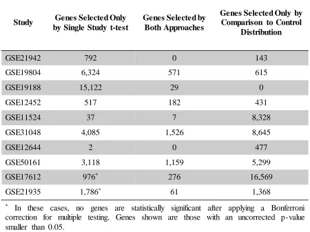
change the resulting groups. ... 48 Table 3.2 Number of Genes Identified by Each Method. Table 3.2 compares the
number of genes that were found to have significantly different
expression between case and control groups of one study by a t-test at a significance level of 0.05 after Bonferroni correction to the number of genes for which the mean expression measurement in the disease group was in the upper or lower 5% of the control reference distribution. For each study, we show the number of genes uniquely identified by each
ix Table S.1 Microarray Datasets Included in Chapter 2 Analyses. This table
summarizes all studies included in the baseline distributions of gene expression measurements in chapter 2 analyses. Studies were separated into the phenotypic subgroups listed above. All datasets, including raw data, experimental design, and sample information, may be found by their accession number at the National Center for Biotechnology Information’s Gene Expression Omnibus (http://www.ncbi.nlm.nih.gov/geo/). In some cases, one or more phenotypic subgroups were excluded from a dataset due to sample size. Only the subgroups listed here were included in
analysis. ... 72 Table S.2 Microarray Datasets Included in Chapter 3 Analyses. This table lists
all studies included in the control reference group in chapter 3 analyses. Only control individuals were taken from these studies. All datasets, including raw data, experimental design, and sample information, may be found by their accession number at the National Center for Biotechnology Information’s Gene Expression Omnibus
(http://www.ncbi.nlm.nih.gov/geo/). ... 75 Table S.3 Microarray Datasets Included in Chapter 4 Analyses. This table
summarizes studies included in chapter 4 analyses. Additionally, all studies included in chapter 2 reference set, summarized in table S.1, were included in chapter 4 work. Studies were separated into the phenotypic subgroups listed above. All datasets, including raw data, experimental design, and sample information, may be found by their accession number at the National Center for Biotechnology Information’s Gene Expression Omnibus (http://www.ncbi.nlm.nih.gov/geo/). In some cases, one or more phenotypic subgroups were excluded from a dataset due to sample size.
x List of Figures
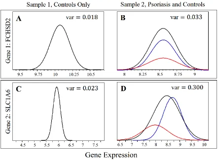
Figure 2.1 Variance in Expression of a Differentially Expressed Gene. Gene expression profiles, fit with normal distributions, are shown for the FCHSD2 gene within A. the controls only from an arthritis study [7] and B. a psoriasis study [6] and the SLC1A6 gene within C. the controls only from the arthritis study and D. a psoriasis study. Note that the scale is equal for panels A and B and for panels C and D, but different across the two genes. For the psoriasis study, the black curve represents all
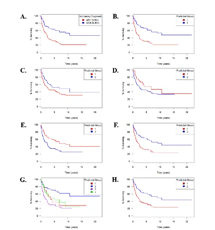
individuals, the red curve represents only the affected (lesional) psoriasis individuals, and the blue curve represents the controls and unaffected skin from psoriasis individuals combined. Variances are shown for the control group in panels A and C and for all individuals in panels B and D. ... 29 Figure 2.2 Comparing Survival of Predicted DLBCL Groups. For the Diffuse
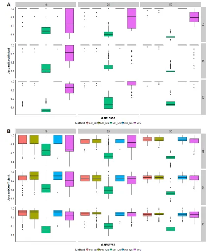
Large B-Cell Lymphoma Study, survival curves are shown for A. the groups described by Alizadeh et al. [2] and the groups resulting from B. SVM, C. NMF, hierarchical clustering using D. all genes, E. the top ten principal components, and F. only genes selected by the proposed method, and model-based clustering using only selected genes, both G. allowing the number of groups to be chosen by the mclust [9] procedure and H. specifying a priori that there were two groups present. ... 30 Figure 2.3 Accuracy to Detect Groups within Study Subsets. Boxplots are shown
for the 500 random subsets at each combination of group sizes for A. the psoriasis study (GSE13355) and B. the kidney cancer study (GSE53757). Points are shown only for outliers... 33 Figure 2.4 Accuracy to Detect Simulated Groups. Boxplots are shown for the 500
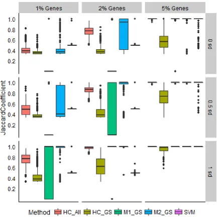
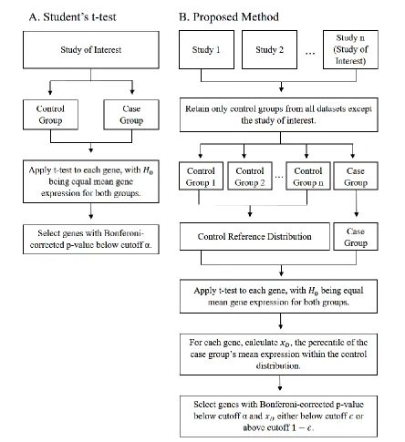
simulated datasets at each combination of effect size and percentage of genes differentially expressed. Points are shown only for outliers. Effect sizes were randomly selected from a normal distribution with mean proportional to the overall standard deviation (sd) of the control group of the psoriasis study. ... 34 Figure 3.1 Comparing the Proposed Method to a Traditional t-test. Workflows
are shown for A. a standard t-test comparing a case and control group from a single study and B. the proposed method comparing a case group of interest to a control reference group drawn from multiple external
xi Figure 4.1 Examining Correlation Distributions for Selected Pairs of Genes.
Density curves summarizing the correlation of expression values for all pairwise combinations of 25 genes from PI(3)K/RTK/RAS pathway. Each curve is a smoothed density of expression correlations within
experimental groups for a single pair of genes. ... 63 Figure 4.2 Examining Correlation Distributions for Identified Gene Pairs with
Highly Correlated Expression. Density curves summarizing the correlation of expression values for each of 6 genes from
PI(3)K/RTK/RAS pathway, the 25 genes having the highest correlation in expression. Each curve is a smoothed density of expression correlations
within experimental groups for a single pair of genes... 64 Figure 4.3 Changes in the Expression Correlation of a Pair of Genes. Simulated
data showing examples of possible differences in the correlation of expression values for a pair of genes between a case and control group. The x and y axes represent centered expression values of two different genes, with each point being a single individual. Black points represent healthy controls and red point represent individuals with a specific disease. Four situations of interest are demonstrated here: A. positive correlation in normal individuals but negative correlation in individuals with certain phenotypes, B. positive correlation in normal individuals but correlation close to zero in individuals with certain phenotypes, C. negative correlation in normal individuals but positive correlation in individuals with certain phenotypes, and D. negative correlation in
normal individuals but correlation close to zero in individuals with certain phenotypes. ... 65 Figure 4.4 Distribution of Within-Group Correlation Values for Selected Gene
xii Figure S.1 Full Results of Random Gene Selection. As an additional evaluation of
1
Chapter 1
Introduction and Background
1.1 Introduction
The amount of genomic data available in public repositories, such as the Gene Expression Omnibus (GEO), has grown exponentially in the past ten years [1]. GEO currently holds over 2 million samples from nearly 80,000 datasets. More than 3,500 species are represented, with human data alone accounting for over 1.1 million samples. GEO has been widely used as a source of test data to evaluate new methods [2-4] and to validate published findings [5-7]. With many phenotypes and tissue types represented, publicly available data can help provide a better understanding of genetic variation on a large scale.
Here, we propose several approaches to integrate public gene expression data with the aim of answering interesting questions in new ways. Though the work of this dissertation focuses on human microarray data, methods can be easily adapted for data from other organisms and technologies if studies are publicly available.
1.2 Prior Results in Data Integration
2 20,000 pairs of genes that are coexpressed, each conserved across species [8]. Evolutionary conservation of coexpression provides strong evidence of a functional relationship between identified genes [8]. Su et al. compared expression of orthologous genes within 16 tissues in mice and humans, finding that some ortholog pairs had very different expression patterns across species. This suggests divergence of biological function across evolution [9]. This work was later extended to a create a gene annotation resource, available at BioGPS (www.biogps.org) [10]. BioGPS is most useful if interested in specific genes rather than doing exploratory analysis. Huang et al. developed a Bayesian approach to use GEO as a diagnostic tool, assigning the most likely phenotype to an individual by identifying similar gene expression profiles in the public repository [11].
3 subscription [13]. The cBio Cancer Genomics Portal, developed at Memorial Sloan-Kettering Cancer Center, was designed to translate the rapidly growing amount of genomics data into clinically relevant information. The database focuses on cancer phenotypes and includes many data types, including mutation, copy number alterations, DNA methylation, and protein levels, and integrates clinical data such as survival information [14]. G-DOC Plus is a data integration and bioinformatics platform which currently holds data from over 10,000 patients from both public and private resources. Tools include differential expression analysis, heat maps, hierarchical clustering, principal component analysis (PCA), survival analysis, a genome browser, and pathway enrichment, though not all tools are available for each sample [15]. For many of these resources, exploratory analysis is difficult without searching for a specific gene or set of genes and the types of analyses that can be performed are limited. In this dissertation, we propose a framework that attempts to address existing questions in novel ways.
1.3 Novel Approaches to Integrate Public Gene Expression Data
In the following chapters, we present three bioinformatics methods that leverage the data contained in genomics repositories to compare gene expression across multiple phenotypes and tissues. Each chapter examines a different summary statistic of gene expression measurements: variance, mean, and correlation.
1.3.1 Variance of Gene Expression
4 within our data. For example, a population of patients diagnosed with the same disease may display variable treatment response or survival time. Without prior knowledge of disease subtypes, can we identify the presence of subgroups and assign group membership to everyone in our study?
In chapter 2, we present a procedure to detect such cryptic subgroups by integrating information from public gene expression studies taken from GEO. First, we propose a novel gene selection method that aims to reduce the dimensionality of our dataset of interest by selecting a set of genes that is enriched for genes that are differentially expressed across the unknown subgroups. External data is used to establish a baseline of variance in expression measurements for each gene. Once we have estimated the amount of expression variance for each gene within a collection of experimental groups, we can determine which genes have large relative variance within our study. This approach is based on the assumption that a gene that is differentially expressed across unknown groups will have higher variance than that same gene in a homogeneous group. Group membership can be predicted using any clustering method, based on only the genes with the most extreme variance relative to the baseline. We show results for 11 test studies as well as simulated data.
1.3.2 Mean of Gene Expression
5 In chapter 3, we demonstrate a method to discover genes that are differentially expressed across phenotypic groups. By integrating external control data, we can identify genes that are associated with a phenotype even in the absence of control data within the study of interest. Rather than compare two groups within a single study (for example, a disease phenotype vs. healthy controls), we compare a disease group of interest to a set of controls from external studies using an unequal variance t-test. In addition to selecting for significant p-values, we impose an additional criterion that genes must have mean expression in the disease group that lies in the upper or lower 5% of the external set of controls. To evaluate the genes selected, we cluster individuals based on the subset of identified genes and compare predicted groups to known groups. We show results for ten test studies. In addition, we apply the proposed approach to five independent lung cancer studies to determine the repeatability of results.
1.3.3 Correlation of Gene Expression
Finally, suppose two genes have correlated expression under most conditions. If that correlation changes within a specific phenotypic group, can this tell us anything about gene function?
6 information about genotype-phenotype relationships. We summarize results for 450 gene pairs.
1.3.4 Conclusions
7 References
1. Edgar R, Domrachev M, and Lash AE: Gene Expression Omnibus: NCBI gene expression and hybridization array data repository. Nucleic Acids Res 2002, 30(1):207-10.
2. Emig D, Ivliev A, Pustovalova O, Lancashire L, Bureeva S, Nikolsky Y, and Bessarabova M: Drug target prediction and repositioning using an integrated network-based approach. PLOS ONE 2013, 8(4):e60618.
3. Gottlieb A, Stein GY, Ruppin E, and Sharan R: PREDICT: a method for inferring novel drug indications with application to personalized medicine. Mol Syst Biol 2011, 7:496.
4. McCall MN, Bolstad BM, and Irizarry RA: Frozen robust multiarray analysis (fRMA). Biostat 2010, 11(2):242-53.
5. Ioannidis JPA, Allison DB, Ball CA, Coulibaly I, Cui X, Culhane AC, Falchi M, Furlanello C, Game L, Jurman G, Mangion J, Mehta T, Nitzberg M, Page GP, Petretto E, and van Noort V: Repeatability of published microarray gene expression analyses. Nat Gen 2009, 41:149-55.
6. de Jonge HJM, Fehrmann RSN, de Bont ESJM, Hofstra RMW, Gerbens F, Kamps WA, de Vries EGE, van der Zee AGJ, te Meerman GJ, and ter Elst A: Evidence based selection of housekeeping genes. PLOS ONE 2(9):e898.
7. Monzon FA, Lyons-Weiler M, Buturovic LJ, Rigl CT, Henner WD, Sciulli C, Dumur CI, Medeiros F, and Anderson GG: Multicenter validation of a 1,550-gene expression profile for identification of tumor tissue of origin. J Clin Oncol 2009, 27(15):2503-8.
8. Stuart JM, Segal E, Koller D, and Kim SK: A gene-coexpression network for global discovery of conserved genetic modules. Science 2003, 302(5643):249-55.
8 10. Wu C, Orozco C, Boyer J, Leglise M, Goodale J, Batalov S, Hodge CL, Haase J, Janes
J, Huss JW III, and Su AI: BioGPS: an extensible and customizable portal for querying and organizing gene annotation resources. Genome Biol 2009, 10:R130. 11. Huang H, Liu CC, and Zhou XJ: Bayesian approach to transforming public gene
expression repositories into disease diagnosis databases. PNAS 2010, 107(15):6823-8.
12. Zhang M, Zhang Y, Liu L, Yu L, Tsang S, Tan J, Yao W, Kang MS, An Y, and Fan X: Gene Expression Browser: large-scale and cross-experiment microarray data integration, management, search, & visualization. BMC Bioinf 2010, 11:433.
13. Hruz T, Laule O, Szabo G, Wessendorp F, Bleuler S, Oertle L, Widmayer P, Gruissem W, and Zimmermann P: Genevestigator v3: a reference expression database for the meta-analysis of transcriptomes. Adv Bioinformatics 2008, 42074.
14. Cerami E, Gao J, Dogrusoz U, Gross BE, Sumer SO, Aksoy BA, Jacobsen A, Byrne CJ, Heuer ML, Larsson E, Antipin Y, Reva B, Goldberg AP, Sander C, and Schultz N: The cBio Cancer Genomics Portal: An Open Platform for Exploring Multidimensional Cancer Genomics Data. Cancer Discov 2012, 2(5):401-4.
9
Chapter 2
Comparing variance in gene expression across a
collection of public studies to reduce data
dimensionality prior to clustering
Rachel L Spreng and Dahlia M Nielsen Under Review by BMC Bioinformatics
2.1 Abstract
11
2.2 Introduction
When performing gene expression studies, often phenotypic subgroups or treatment groups are known and the goal is to find genes that are differentially expressed across those groups. Here we are instead operating under the premise that unknown subgroups are present in a dataset, and our goal is to identify these subgroups and assign group membership to the individuals in the study. For example, patients with the same disease diagnosis may be variable in symptoms, severity, or treatment response. It would be beneficial to know if those different responses reflect distinct subtypes of the disease, as this would aid in diagnosing and treating patients. Discovery of subgroups is not a novel idea – many methods exist for this purpose (for a review and comparison study, see [1]).
A commonly used method is hierarchical clustering, which can be applied to many types of data and is efficient for high dimensional data. However, determining the appropriate number of subgroups present in the data is a challenge. Model-based clustering addresses this problem by estimating the number of clusters based on the data, but is less efficient on large datasets.
12 different overall survival. While this method was effective in identifying subgroups of DLBCL, it is highly specific to that disease. Without knowledge about the genes involved in a trait of interest, this approach would not be useful.
As an alternative to gene selection, some methods reduce the dimensionality of a dataset by summarizing all genes using a small number of metagenes. For example, principal component analysis (PCA) identifies linear combinations of genes, called principal components (PCs), that represent the complete set of genes. Typically, the first few PCs capture most of the variation in gene expression and therefore are assumed to be sufficient for clustering. By plotting one PC vs another, clusters of the observations can often be identified visually. Though this is subjective, it can be a good way to estimate the number of subgroups present in a dataset. For an unbiased approach, clustering methods can be applied to a small set of top PCs instead of to all genes. PCA is computationally efficient and easily implemented. However, the first few PCs do not always capture the biological signal of interest and some studies, such as [3], have reported that clustering on PCs rather than the expression of all genes does not improve ability to detect known groups.
Similarly, non-negative matrix factorization (NMF) methods reduce all genes into only a few metagenes, linear combinations of all genes. The 𝑛×𝑚 data matrix A, where 𝑛 is the total number of genes and 𝑚 is the sample size, is factored into the 𝑛×𝑘 matrix W, where
𝑘 is the number of metagenes and 𝑤𝑖𝑗 is the coefficient of gene 𝑖 in metagene 𝑗, and the 𝑘×𝑚
13 expression in the corresponding metagene is highest. NMF can be computationally intensive. Additionally, there are often multiple solutions to the factorization A= WH, and thus results are not always reproducible. For a more complete description of NMF, see [4].
This is not an exhaustive list of subgroup discovery methods, but we feel that it represents a wide range of available approaches. Each has its own advantages and disadvantages, and any method will perform differently depending on the features of the dataset. Many existing methods for subgroup identification require prior knowledge, a training dataset, or specification of multiple parameters. In addition, most methods require the number of clusters to be chosen a priori, though this information is likely unknown. Here, we present a method which requires no parameters or prior knowledge, is applicable to any gene expression study, and is straightforward to use.
2.3 Results and Discussion
14 NCBI GEO database, accessions GSE13355 and GSE13501, respectively) [5-7]. Study-wide variance in expression measurements is not significantly different between the two datasets for the gene FCHSD2 (Affymetrix Probe ID 203620_s_at), and this gene does not appear to be differentially expressed across conditions in the psoriasis dataset. The gene SLC1A6 (Affymetrix Probe ID 1554593_s_at), however, has a significantly higher variance in expression measurements from the whole psoriasis dataset relative to the controls of the arthritis study. When differential expression analysis was performed across the subgroups of the psoriasis study, SLC1A6 was one of the genes identified.
As some genes naturally have higher variance in their expression than others, purely selecting the genes with the highest variance in expression measurements within a study is not ideal, especially given that additional information is available. Instead, genes displaying significantly higher variance in expression measurements within the dataset of interest compared to external studies are chosen for subgroup identification. Once the dimensionality of the data is reduced by gene selection, individuals within the dataset of interest can be clustered based on expression measurements for the chosen genes.
2.3.1 Biological Studies
15 proposed method to this dataset, survival time and Alizadeh’s DLBCL subtype diagnosis
were available, both of which served as a test of the results of this method. It is important to note that the published subgroups [2] were not confirmed via independent assays, thus perfect correspondence with these subtypes is not necessarily the optimal outcome. Rather, we evaluated the effectiveness of each approach based on how differentiated the resulting subgroups were in terms of their survival times.
16 against a more informed method. Though other subgroup discovery methods are available, these methods were chosen as representatives because they are well defined, easily implemented, and vary in the amount of information required a priori. For more information about each approach, see the Methods section. For the dataset of Alizadeh et al. [2], Figure 2.2 shows survival curves for subgroups identified by each of these methods. Table 2.1 summarizes the mean survival times and p-values for tests of difference in survival across these subgroups.
For this dataset, SVM produced the groups with the biggest difference in survival, which is unsurprising, since more information is provided a priori to SVM than to the other methods being compared. Applying the log-rank test for difference between survival curves, the p-value for the groups identified by SVM is 8.97×10⁻⁶, while the p-value for the groups
published by Alizadeh et al. is 4.69×10⁻⁵. Nonnegative matrix factorization produced
groups that do not have significantly different mean survival time, with a p-value of 0.297. Hierarchical clustering using all genes also produced groups whose survival times were not significantly different from each other (p-value 0.132) and which have high discordance with the groups produced by Alizadeh et al. However, when the proposed gene selection method was applied to the data, and the genes selected subjected to hierarchical clustering, the resulting groups had significantly different mean survival (p-value 3.14×10⁻⁴).
17 When individuals were clustered by the mclust package with no prior specification regarding the number of subgroups, mclust estimated that there were four groups present in the data (groups A1-A4; Fig. 2.2E). The p-value for the test for differences between survival curves for these four groups is 2.01×10⁻⁴. Further study would be necessary to determine if there is biological significance to all four groups, but we can see a significant difference in survival between groups A2 and A3 (Fig. 2.2E). When the number of subgroups was chosen a priori to be two (groups B1 and B2; Fig. 2.2F), the p-value measuring the difference between survival curves of those two groups was 3.86×10⁻⁴. With the exception of three
individuals, group B1 is a combination of groups A1 and A3 and group B2 is a combination of groups A2 and A4. All results from mclust were obtained by clustering individuals based on the subset of genes identified by our gene selection approach.
18 The Jaccard Similarity index, 𝐽, was used to measure the concordance between the subgroups identified by each method and the true subgroups. J is defined to be the proportion of pairs of individuals that are grouped together in both the known groups and the predicted groups. It has a minimum of zero and reaches a maximum of one when known and predicted groups have perfect concordance. For a discussion of the advantages of this test statistic compared with other accuracy measures, see the Methods section.
For six of the test datasets, either model-based clustering or hierarchical clustering combined with the proposed gene selection method performed as well or better than clustering on all genes. For an additional two datasets, the proposed gene selection method combined with at least one clustering method resulted in groups that were reasonably close those of the best performing method (𝐽 within 0.1). NMF best predicted known groups in two cases, though NMF results are often non-unique and are thus not reproducible. This method often placed all individuals in a single group, so NMF was run iteratively for each dataset until a non-trivial result was identified.
19 genes showed a fold change greater than 2. If effect sizes of differentially expressed genes are predominantly small within a population of interest, the proposed selection method is unlikely to identify those genes.
For dataset GSE53757, the Jaccard coefficient 𝐽 was consistently high for the groups resulting from all methods, with very little variation in 𝐽 between the repetitions of random gene selection prior to clustering. One explanation for consistently large values of 𝐽 is that a number of genes in the study are differentially expressed across groups with reasonably large effect sizes. Again, we applied a t-test to this dataset, and found that nearly half of the genes had significantly different mean expression between the control and clear cell renal cell carcinoma groups (results not shown). While no genes showed fold change greater than two, effect sizes were larger than in the previous case. In this dataset, differences in gene expression were widespread and relatively large, so any method would likely capture the true groups. In addition, this study was comprised of matched tumor and control samples, which eliminates some of the confounding factors that may be seen in other studies. The only method that did not produce subgroups with high concordance to known subgroups for this dataset was model-based clustering when the number of groups was selected by the model; this approach over-fit the data by choosing 5 groups.
20 groups showed that nearly 20% of genes had significantly different mean expression between the control group and at least one of the irritable bowel syndrome (IBS) subgroups, with relatively small fold change values (results not shown). No genes were significantly differentially expressed between the two IBS subgroups. Even applying the above methods to only the two IBS subgroups, removing control individuals, most methods places all (or a large majority) of the IBS individuals in a single group. Hierarchical clustering on the top ten principal components produces the groups with the highest concordance to known groups, having an accuracy of 0.422. For this dataset, gene expression differences between the IBS subtypes are seemingly too small to detect using any method tested.
2.3.2 Simulated Data
21 versus normal skin) [6]. Nine sets of group sizes were tested – all combinations of sample sizes 10, 25, and 50 (see Methods). This set of group sizes was chosen to give a representation of larger and smaller overall sample sizes, as well as balanced and unbalanced group sizes. Results are presented in Figure 2.3. Though more information is provided to SVM a priori, this approach resulted in smaller values of 𝐽 and more variation between repetitions than the other methods, especially when group sizes were small or unbalanced. Model-based clustering failed to predict the number of known groups in most cases, resulting in small values of 𝐽. Gene selection combined with either hierarchical or model-based clustering often produced results as good as or better than hierarchical clustering on all genes, even for small overall sample size or unbalanced group sizes.
Next, we simulated data from a normal distribution based on the mean and standard deviation from the control individuals of the psoriasis study [6]. This allowed us to control how many genes were differentially expressed and how large their effect sizes were. The probability of a gene being selected to be differentially expressed was either 1%, 2%, or 5%. If differential expression was simulated for a gene, the effect size was chosen from a normal distribution with a mean equal to the standard deviation of expression measurements for that gene within the control group of the psoriasis study multiplied by either 0, 0.5, or 1 (see Methods). All possible combinations of these values were tested. Results are shown in Figure 2.4.
22 groups that had increasing concordance with known groups as the percentage of genes differentially expressed increased, while gene selection combined with either clustering method was more helpful as effect sizes increased. SVM did not capture known groups well when fewer genes were differentially expressed, except when the effect size multiplier was at its largest tested value. Though this information will not be known a priori, the proposed gene selection method is most likely to improve subgroup discovery results if effect sizes are larger, especially in cases where few genes are differentially expressed.
2.4 Conclusions
Discovery of cryptic subgroups of individuals within a population of interest is challenging, but it is valuable in advancing scientific understanding of that population. For example, the ability to classify survival differences could allow clinicians to better evaluate patient prognosis, and further investigation of the biological differences between low and high survival groups could lead to improved treatment. The high dimensionality of gene expression data, however, often presents a challenge when using traditional clustering techniques. Here, we have proposed a method that uses a gene selection step designed to reduce the data to a subset enriched for informative genes prior to clustering of individuals.
23 effects) or unobserved biological factors, or they could be artifacts. If the proposed gene selection step is combined with model-based clustering without specifying the number of groups a priori, results should be carefully considered. In simulations, the accuracy of mclust in selecting the number of groups increased as both the number of genes differentially expressed increased and their effect sizes increased.
Applying the proposed gene selection method to the Diffuse Large B-Cell Lymphoma study significantly improved hierarchical clustering results. Though SVM produced the groups with maximal difference in survival, this method is not an option in the absence of prior knowledge of subgroups. Each clustering method combined with the proposed gene selection technique was able to produce groups with significantly different survival times, though p-values were smaller than those corresponding to Alizadeh’s groups or SVM results. However, the proposed gene selection method, combined with the clustering method of choice, requires no prior knowledge and is not disease-specific.
24 Simulations demonstrated that gene selection is most helpful when the amount of differential expression between groups is large, regardless of how many genes are differentially expressed. Hierarchical clustering using all genes is expected to produce the best groups if a large proportion of genes are differentially expressed across groups, with most genes having small effect sizes. Despite the fact that more information is provided a priori, SVM did not typically perform as well as unsupervised methods when group sizes were small.
Though the gains of gene selection were sometimes small, there are additional benefits to the proposed gene selection technique. Including all genes in an analysis is not always computationally tractable, especially when using a model-based clustering approach. Randomly selecting genes is not ideal, since results will be highly dependent upon which genes are chosen, and results are not necessarily reproducible. The method proposed here is recommended if it is not feasible to use all genes in the analysis, or if clustering on all genes produces results which do not agree with experimental observations.
25 two other datasets is an option when applied to organisms or technologies for which few studies are available.
2.5 Method Details
Establishing baseline gene expression variance
In order to select the genes most likely to be involved in the grouping of interest, the proposed method compares the variance in expression measurements for each gene within the study of interest to a baseline variance. To establish a baseline for gene expression variance, 53 datasets from human studies were chosen from NCBI’s Gene Expression
Omnibus (GEO) and divided into 108 subsets, each consisting of patients with the same known disease status. Within the Affymetrix Human Genome U133 Plus 2.0 Array platform, three criteria were used for the selection of reference datasets.
1. Data was published no earlier than 2008 2. Total sample size was between 20 and 250 3. All subset sample sizes were 10 or greater
For datasets containing multiple subsets, only those subsets satisfying criterion (3)
were included. For a complete list of the datasets and subsets used, see Appendix B. Note that when a dataset from this collection was used for methods testing, all subsets from that study were removed from the baseline distribution.
Gene Expression Pre-Processing and Normalization
26 GEOquery package [15]. The microarray gene expression data were log2 transformed prior to normalization. All datasets were normalized independently and identically using Loess normalization, implemented in the affy package [16]. Loess normalization [17] is based on the M vs. A plot, where M is the difference in log expression values and A is the average of the log expression values. For each possible pairwise combination of arrays (corresponding to individuals), a local regression is fit to the M vs. A plot and 𝑀𝑘, where 𝑘 = 1,2, … , 𝑝
indicates the probe, is adjusted by subtracting the fitted value. After normalization, the expression of each RNA target is summarized as the mean of the log2 transformed, loess normalized probes.
As a quality control step, JMP Genomics Distributional Analysis [18-19] was performed on the eleven biological datasets used to test the method, with outliers removed. This resulted in the exclusion of four individuals from three different datasets (GSM161943 and GSM161944 from GSE7014, GSM899127 from GSE36701, and GSM1300092 from GSE53757).
Gene Selection
27 expression variance in the test set that was greater than at least 95% of reference variances were selected for subgroup identification. We chose to use this approach rather than apply a statistical test for several reasons. After evaluating several parametric and non-parametric tests to compare a dataset of interest to the reference control (results not shown), most tests selected too many genes. The reference set being significantly larger than any test dataset is a concern when applying these tests. In addition, by using our metric, we avoid making any distribution assumptions about the data.
Subgroup Identification
28 Simulation
In order to test the method under different circumstances, we generated simulated data. Two simulation approaches were implemented. For the first approach, two studies were used, a psoriasis dataset (data accessible at NCBI GEO database, accession GSE13355) [5,6] and a dataset consisting of clear cell renal cell carcinoma tissue versus matched normal kidney tissue (data accessible at NCBI GEO database, accession GSE53757) [13]. Two subsets were extracted from the psoriasis dataset: healthy control tissue and affected psoriasis tissue. For each dataset, the protocol was the same: random subsets of samples were chosen containing 10, 25, or 50 individuals from each of the two groups of data. For each possible combination of group sizes, 500 random subsets were chosen.
Approach 2 protocol was implemented as follows:
1. For each gene, 200 expression measurements were generated from a normal distribution. The mean and standard deviation of the distribution used to generate expression measurements was equal to those of the control individuals from the psoriasis study mentioned previously.
2. Individuals were randomly assigned to one of two treatment groups, with 100 individuals in each group.
29 4. If a gene was chosen to be differentially expressed, the expression values for
one group were chosen from a normal distribution,
N(𝜇 = 𝜇𝑁𝑁 +N(𝑒, 0.5)×𝑠𝑑𝑁𝑁, 𝑠𝑑 = 𝑠𝑑𝑁𝑁),
where 𝜇𝑁𝑁 and 𝑠𝑑𝑁𝑁 are the mean and standard deviation, respectively, of expression measurements in the control individuals of the psoriasis study and
𝑒 is an effect size multiplier variable, equal to 0, 0.5, or 1.
For each possible combination of the variables in steps 3 and 4, the simulation was repeated 500 times.
Comparison Methods
30 SVM, implemented using the R package kernlab [9,12], using half of the individuals to train the model and clustering the remaining half based on that model.
Evaluation of Results
For the Diffuse Large B-Cell Lymphoma study, results were evaluated based upon how different the groups identified by the various methods were in terms of survival. The log-rank test was used to obtain a p-value for difference between survival times.
For all other comparisons between methods, the test statistic used to assess the significance of the groups identified was the Jaccard Similarity Coefficient, 𝐽. The Jaccard Coefficient has a minimum of zero and a maximum of 1 (when predicted groups exactly match known groups). This measure of accuracy is quite conservative and is sensitive to differing numbers of known and predicted groups, unbalanced group sizes, and overall sample size. Though these sensitivities make comparing results across studies difficult, the Jaccard Coefficient is a good measure of different methods applied to the same study. It is an ideal test statistic because it does not require subjective decisions concerning which known groups and predicted groups correspond to one another. It can also be calculated for any number of groups. 𝐽 is equal to the proportion of individual pairs which are grouped together in both the known groups and the predicted groups, and is defined as
𝐽 = ∑ ∑ (𝑛𝑘𝑝 2 ) 𝑃 𝑝=1 𝐾 𝑘 =1 ∑ ∑ (𝑛𝑘𝑝 2 ) 𝑃 𝑝=1 𝐾
𝑘 =1 + ∑𝐾𝑘=1∑𝑃𝑝=1[𝑛𝑘𝑝(∑𝐾𝑟 =𝑘+1𝑛𝑟𝑝+ ∑𝑃𝑐=𝑝+1𝑛𝑘𝑐)]
,
33 Table 2.1 Summary of Diffuse Large B-Cell Lymphoma (DLBCL) Results. Summary of group sizes (subset by group label as defined by Alizadeh et al.), mean survival time, 𝑡̅ (in years), and p-value for the test of difference in survival of the groups resulting from each method. For reference, Alizadeh et al.’s groups have a p-value of 4.69×10⁻⁵, with the
GCB-DLBCL group having a mean survival time of 6.78 years and the ABC-DLBCL group having a mean survival time of 3.09 years. Group labels by the various methods are arbitrary, thus group 1 resulting from one method does not necessarily correspond to group 1 resulting from any other method.
M ethod p-value Properties
Predicted Group
1 2 3 4
M odel-Based
(Approach A) 2.01×10
−4
𝑡̅ (years) 3.77 7.42 2.89 4.80
𝑛GCB 8 47 0 20
𝑛ABC 9 5 60 0
M odel-Based
(Approach B) 3.86×10
−4
𝑡̅ (years) 3.20 6.63
𝑛GCB 7 68
𝑛ABC 69 5
Hierarchical
(All Genes) 1.32×10
−2
𝑡̅ (years) 6.37 4.43
𝑛GCB 25 50
𝑛ABC 8 66
Hierarchical
(Gene Selection) 3.14×10
−4
𝑡̅ (years) 3.15 6.62
𝑛GCB 8 67
𝑛ABC 66 8
Hierarchical
(Top PCs) 2.35×10
−3
𝑡̅ (years) 6.29 3.22
𝑛GCB 64 11
𝑛ABC 17 57
SVM 8.90×10⁻⁶
𝑡̅ (years) 2.98 6.93
𝑛GCB 2 73
𝑛ABC 67 7
NM F 6.26×10⁻²
𝑡̅ (years) 4.30 6.25
𝑛GCB 44 31
34 Table 2.2 Summary of Results on Biological Studies. Summary of the results of various methods on 10 biological datasets (labeled by their GEO accession number). Shown are the calculated values of the Jaccard Similarity Coefficient, 𝐽, a measure of concordance between known groups and the groups predicted by different methods. For the clustering methods applied to randomly selected genes, 𝐽 is a mean from 500 iterations and the standard deviation of the 𝐽 measure from those iterations is in parentheses.
Model-Based Clustering Hierarchical Clustering SVM NMF
Dataset Gene Selection Gene Selection (Specify # of groups) 1000 Random Genes Selected All Genes Gene Selection Principal Components 1000 Random Genes Selected All Genes All Genes
GSE10245 0.464 0.797 0.707
(0.113) 0.843 0.797 0.641
0.716
(0.121) 0.543 0.402
GSE10334 0.259 0.508 0.391 (0.005) 0.716 0.471 0.388 0.530 (0.126) 0.646 0.392
GSE22377 0.769* 0.769 0.637 (0.103) 0.665 0.713 0.359 0.642 (0.106) 0.696 0.769
GSE28571 0.391 0.378 0.413
(0.070) 0.473 0.391 0.311
0.418
(0.063) 0.445 0.549
GSE13911 0.410* 0.410 0.483
(0.090) 0.383 0.411 0.400
0.445
(0.103) 0.565 0.379
GSE16581 0.246 0.404 0.405
(0.026) 0.404 0.404 0.400
0.402 (0.015) 0
** 0.397
GSE11524 0.212 0.422 0.425
(0.040) 0.422 0.422 0.455
0.431
(0.037) 0.566 0.446
GSE36701 0.334 0.300 0.301
(0.022) 0.272 0.302 0.269
0.292
(0.013) 0.334 0.312
GSE53757 0.520 0.872 0.811
(0.012) 0.872 0.872 0.828
0.860
(0.032) 0.944 0.849
GSE7014 0.402* 0.402 0.569 (0.053) 0.582 0.402 0.384 0.558 (0.070) 0** 0.339
*
Indicates that the model-based clustering procedure predicted the correct number of groups.
37 References
1. Dudoit S, Fridlyand J, Speed TP: Comparison of Discrimination Methods for the Classification of Tumor Using Gene Expression Data. J Am Stat Assoc 2002, 97(457):77-87.
2. Alizadeh AA, Eisen MB, Davis RE, Ma C, Lossos IS, Rosenwald A, Boldrick JC, Sabet H, Tran T, Yu X, Powell JI, Yang L, Marti GE, Moore T, Hudson J Jr, Lu L, Lewis DB, Tibshirani R, Sherlock G, Chan WC, Greiner TC, Weisenburger DD, Armitage JO, Warnke R, Levy R, Wilson W, Grever MR, Byrd JC, Botstein D, Brown PO, Staudt LM: Distinct types of diffuse large B-cell lymphoma identified by gene expression profiling. Nature 2000, 403:503-11.
3. Yeung KY and Ruzzo WL: Principal component analysis for clustering gene expression data. Bioinformatics 2001, 17(9):763-74.
4. Brunet JP, Tamayo P, Golub TR, and Mesirov JP: Metagenes and molecular pattern discovery using matrix factorization. PNAS 2004, 101(12):4164-9.
5. Edgar R, Domrachev M, Lash AE: Gene Expression Omnibus: NCBI gene expression and hybridization array data repository. Nucleic Acids Res 2002, 30(1):207-10.
6. Nair RP, Duffin KC, Helms C, Ding J, Stuart PE, Goldgar D, Gudjonsson JE, Li Y, Tejasvi T, Feng BJ, Ruether A, Schreiber S, Weichenthal M, Gladman D, Rahman P, Schrodi SJ, Prahalad S, Guthery SL, Fischer J, Liao W, Kwok PY, Menter A, Lathrop GM, Wise CA, Begovich AB, Voorhees JJ, Elder JT, Krueger GG, Bowcock AM, Abecasis GR: Genome-wide scan reveals association of psoriasis with IL-23 and NF-kappaB pathways. Nat Genet 2009, 41(2):199-204.
7. Barnes MG, Grom AA, Thompson SD, Griffin TA, Pavlidis P, Itert L, Fall N, Sowders DP, Hinze CH, Aronow BJ, Luyrink LK, Srivastava S, Ilowite NT, Gottlieb BS, Olson JC, Sherry DD, Glass DN, Colbert RA: Subtype-specific peripheral blood gene expression pro-files in recent-onset juvenile idiopathic arthritis. Arthritis Rheum 2009, 60(7):2102-12.
38 lymphoma treated with rituximab plus chemotherapy. Haematologica 2011, 96(7):996-1001.
9. R Core Team: R: A language and environment for statistical computing. R Foundation for Statistical Computing, Vienna, Austria. [http://www.R-project.org] 10. Fraley C and Raftery AE: Model-based Clustering, Discriminant Analysis and
Density Estimation. J Am Stat Assoc 2002, 97:611-31.
11. Gaujoux R and Seoighe C: A flexible R package for nonnegative matrix factorization. BMC Bioinformatics 2010, 11:367.
12. Karatzoglou A, Smola A, Hornik K, Zeileis A: kernlab - An S4 Package for Kernel Methods in R. J Stat Softw 2004, 11(9):1-20.
13. von Roemeling CA, Radisky DC, Marlow LA, Cooper SJ, Grebe SK, Anastasiadis PZ, Tun HW, Copland JA: Neuronal pentraxin 2 supports clear cell renal cell carcinoma by activating the AMPA-selective glutamate receptor-4. Cancer Res 2014, 74(17):4796-810.
14. Gentleman RC, Carey VJ, Bates DM, Bolstad B, Dettling M, Dudoit S, Ellis B, Gautier L, Ge Y, Gentry J, Hornik K, Hothorn T, Huber W, Iacus S, Irizarry R, Leisch F, Li C, Maechler M, Rossini AJ, Sawatzki G, Smith C, Smyth G, Tierney L, Yang JYH, Zhang J: Bioconductor: Open software development for computational biology and bioinformatics. Genome Biol 2004, 5:R80.
15. Davis S, Meltzer P: GEOquery: a bridge between the Gene Expression Omnibus (GEO) and BioConductor. Bioinformatics 2007, 14:1846-1847.
16. Gautier L, Cope L, Bolstad BM and Irizarry RA: affy—analysis of Affymetrix
GeneChip data at the probe level.Bioinformatics 2004, 20(3):307-315.
17. Cleveland WS and Devlin SJ: Locally Weighted Regression: An Approach to Regression Analysis by Local Fitting. JASA 1988, 83(403):596-610.
18. JMP, Version 12.0. SAS Institute Inc., Cary, NC.
39
Chapter 3
Comparing mean gene expression across a collection
of public studies to identify differentially expressed
genes
Rachel L Spreng and Dahlia M Nielsen
3.1 Abstract
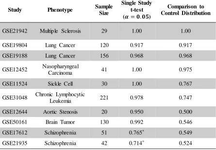
40 measurements from the control groups of many different studies. The phenotype of interest can then be compared to this reference control group rather than being compared only to its corresponding controls. We have applied an unequal variance t-test comparing a target group to our reference control group, imposing the additional condition that a selected gene must have a mean expression in the target study that lies in the extremes of the reference distribution. By taking this approach, gene associations can be identified even in the absence of control data in the study of interest. In most cases, the proposed method successfully identified a subset of genes that sufficiently clustered data into known groups. Though this is not confirmation of association, it does indicate that the set of genes selected is enriched for genes that are differentially expressed between the phenotype of interest and controls. When our method was applied to multiple independent lung cancer studies, there was a set of seven genes that were identified in every case, all of which have some known association with lung cancer or cancer processes in general.
3.2 Introduction
41 commonly chosen to be two. This approach is effective when the genes of interest have large effect sizes but, by design, will not identify genes with smaller amounts of differential expression.
Statistical tests such as analysis of variance (ANOVA) and the student’s t-test can
account for both the fold-change and the variability of gene expression. When applying these tests, the null hypothesis for any given gene is that the groups of interest have equal mean expression of that gene. It is assumed that gene expression values within the sample populations being compared are normally distributed and that the different groups have equal variance in expression measurements, though Welch’s t-test is adapted for unequal variance. Another option is a non-parametric test such as the Kruskal-Wallis test, which makes no assumptions about distribution and is more powerful than parametric tests if the data has heavy tails, is skewed, or contains outliers. ANOVA, the student’s t-test, and the Kruskal-Wallis test all assume that the data was independently sampled from the populations being compared, which is violated if the data was collected in clusters. For further discussion of methods that are commonly used to identify differentially expressed genes, see reviews by Cui et al. and Dudoit et al [1-2].
42 additional information about gene expression levels under control conditions. Here, we have combined the controls from 33 different microarray datasets, obtained from the National Center for Biotechnology Information’s Gene Expression Omnibus (NCBI GEO) database [3], to create an expression distribution for each gene which serves as a baseline for comparison.
3.3 Results and Discussion
We describe a method to identify genes that are associated with a phenotype or trait of interest, even if a control group was not assayed for the study of interest. Our approach is based on comparing the gene expression measurements from individuals that share the trait of interest (e.g. a common disease diagnosis, treatment, etc.) to our set of 1,143 control individuals from 33 studies, taken from GEO. If the study of interest included control individuals, we added those to our reference group. Figure 3.1 compares a typical t-test approach to the method proposed here, which can be used to detect differentially expressed genes for any data, even in the absence of a control group. The proposed method applies a t-test to the study group of interest and the control reference group, but applies an additional condition that the mean expression of any selected gene has expression in the study group which lies in the upper or lower 5% of the control reference group.
43 clustering on the genes identified by each approach. Next, we analyzed five independent lung cancer studies and report the genes that were identified in all five studies.
3.3.1 Accuracy of Clustering on Identified Genes
For ten biological studies (all data accessible at NCBI GEO) [3-13], we have compared (a) a t-test between cases and controls from one study to (b) the proposed method of a t-test between the case group and the control reference distribution, with the additional criterion that a selected gene must have a mean in the case group that lies in the upper or lower 5% of the control distribution.
In each study, the subsets of genes selected by (a) and (b) were used to cluster the individuals of the original dataset as a validation of the genes identified (results presented in Table 3.1). Clustering was performed using a hierarchical clustering approach, implemented using the hclust function in R [14]. Here, we define the accuracy of clustering as the proportion of individuals correctly placed into known groups, where each predicted group is assumed to correspond to the known group to which the majority of its members belong. This measure has a minimum of 0.5 and reaches a maximum of one when known and predicted groups have perfect concordance.
44 genes chosen is not sufficient to discriminate known groups, but is not conclusive evidence that those genes are unrelated to the given phenotype.
For three studies, clustering on the genes selected by the proposed method reproduced known groups with the same accuracy as clustering on the genes selected by a t-test applied to the cases and controls of that study. For one study, the loss in accuracy resulting in clustering on genes selected by the proposed method was small (less than 0.1). For two studies, the loss in accuracy was moderate (less than 0.25). Finally, for four studies, the loss in accuracy was large (greater than 0.25). Three of these four studies involve brain tissue, which may indicate that gene expression within the brain is significantly different than in other tissues, especially since brain tissue is not well represented in our control reference set. Further, two of these studies used postmortem brain tissue, so RNA quality could be a factor. It is possible that the genes identified are associated with the trait of interest, but those genes alone are insufficient to discriminate the data into known phenotypic groups.
45 with high concordance to known groups. The proposed method did not always select fewer genes than a t-test on only the study of interest; however, in most cases where it did, clustering results were as good or within 5% accuracy. Though we cannot confirm without further investigation which genes are associated with the phenotypes of interest, this demonstrates that where fewer genes are selected, the proposed method is not excluding genes which are necessary to discriminate groups. The exception to this is study GSE21936, where the proposed method selects fewer genes, but the set of selected genes is not sufficient to cluster individuals into known groups.
3.3.2 Comparing Results from Multiple Lung Cancer Studie s