FAST PROCESSING INTELLIGENT WIND FARM
CONTROLLER FOR PRODUCTION
MAXIMISATION
Tanvir Ahmad1,2*, Abdul Basit1, Samia Akhtar3, Juveria Anwar1, Olivier Coupiac4, Behzad Kazemtabrizi2and Peter C Matthews2,
1 US Pakistan Center for Advanced Studies in Energy, UET Peshawar Pakistan
2 School of Engineering Durham University, UK
3 Pakistan Council of Renewable Energy Technologies
4 Engie Green France
* Correspondence: [email protected]
Version January 8, 2019 submitted to Preprints
Abstract: A practical wind farm controller for production maximisation based on coordinated 1
control is presented. The farm controller emphasises computational efficiency without compromising 2
accuracy. The controller combines Particle Swarm Optimisation (PSO) with a turbulence intensity 3
based Jensen wake model (TI-JM) for exploiting the benefits of either curtailing upstream turbines 4
using coefficient of power (CP) or deflecting wakes by applying yaw-offsets for maximising net farm 5
production. First, TI-JM is evaluated using convention control benchmarking WindPRO and real 6
time SCADA data from three operating wind farms. Then the optimized strategies are evaluated 7
using simulations based on TI-JM and PSO. The innovative control strategies can optimise a medium 8
size wind farm, Lillgrund consisting of 48 wind turbines, requiring less than 50 seconds for a single 9
simulation, increasing farm efficiency up to a maximum of 6% in full wake conditions. 10
Keywords: wind farm production maximisation, coordinated control, CP-based optimisation, 11
yaw-based optimisation, wake effects, turbulence intensity, Jensen model, particle swarm optimisation 12
1. Introduction 13
Wind farms take advantages of economies of scale for reducing levelised cost of energy by 14
clustering turbines together. However, turbines in this cluster interact with each other aerodynamically 15
through wake effects. Wake effects or simply wakes can significantly impact economic performance of 16
a wind farm by decreasing net production or increasing fatigue loads [1–3]. 17
Industry best practice is to increase the spacing between the turbines in the prevailing wind 18
directions (downwind) as compared to non-prevailing wind directions (crosswind) [2]. Wake losses in 19
the crosswind directions can be as high as 50% due to the close spacing [4], reducing the farm efficiency 20
to as low as 40% [5]. 21
Another way of reducing wake effects is global optimisation of the whole wind farm using 22
coordinated control. With state of the art (greedy control), every turbine maximises its own production, 23
neglecting the wake effects on shadowed turbines [2]. Coordinated control based on global optimisation 24
of the whole wind farm instead of local optimisation of individual turbines can result in increased 25
annual energy production [6]. 26
Coordinated control is the farm level control (termed farm control or optimised control as well), 27
which is based on the optimised cooperation or coordination of turbines in the farm. In such control, 28
turbines coordinate with each other for increasing the net production. Curtailing or yawing the 29
upstream turbines reduces the wake effects produced, hence increasing production of downstream 30
turbines. If decrease in the upstream turbines’ net production is less than increase in the downstream 31
turbines’ net production then the farm net production will increase. 32
A detailed literature review of coordinated control studies in [7,8] concludes that realisation of 33
benefits of coordinated control depends upon terrain characteristics, atmospheric wind conditions, 34
layout of the wind farm and number of turbines under consideration. Wakes recover quickly in rough 35
terrains as compared to smooth surfaces (offshore) [7]. In certain wind directions, downstream turbines 36
are under significant wake effects, impacting their production negatively. Usually negligible wake 37
effects are observed at higher wind speeds in above-rated wind conditions [5]. Net production of 38
denser wind farms (with closely spaced turbines) is generally affected more by wake effects [5]. 39
Coordinated control can be performed with optimal settings ofCP or yaw offsets (α) of the 40
upstream turbines. This requires no additional cost, where the only change required in the existing 41
control system will be the coordinated control algorithm, specifically a change in the software [4,9]. 42
Intelligent farm control aimed at maximising net present value will replace turbine power curve as 43
the main performance characteristic [6]. As real time on-line optimisation is required and given the 44
stochastic nature of wind, the controller must be fast and accurate. Specifically, control updates need to 45
be made in seconds. An optimiser and a wind deficit model (wake model) are required in such setup 46
for coordinated control. The optimiser evaluates different combinations of power productions of the 47
turbines using the wind deficit model for achieving the optimum net production. It shall be noted that 48
there is an inverse relationship between accuracy and computational cost of the farm controller. Real 49
time (online) implementation of coordinated control requires faster (usually in the order of seconds) 50
and accurate control strategies that can cope with stochastic nature of the wind [6,10]. 51
Development of such on-line, accurate and computationally efficient coordinated control strategies 52
for production maximisation is the aim of this paper. Particle Swarm Optimisation (PSO) is combined 53
with a fast processing wind deficit model (TI-JM) for developing a realistic and practical on-line wind 54
farm controller. This work is mainly based on the research carried out in [7]. This paper is structured in 55
different sections, described as follows. A brief overview of TI-JM is given in section2. This is followed 56
by detailing the optimisation process in section3with the control problem and objective function 57
formulation in section3.1and details of PSO in section3.2. Information about the three wind farms: 58
Brazos, SMV and Lillgrund is provided in sections4.1,4.2and4.3respectively. The methodologies 59
for obtaining efficiencies of the farms case studies are discussed in section5. Results and analyses are 60
presented in section6. Conclusion of this work is given in section7. 61
2. Turbulence Intensity based Jensen Model (TI-JM) 62
This section gives a brief overview of TI-JM, which is used for developing the coordinated control strategies. The detailed methodology for developing TI-JM and validation using real-time data is given in [7]. TI-JM modifies the wake decay coefficient (k) of the standard Jensen model [11,12] using wake-added turbulence intensity. Wake decay coefficient presents how quickly the wake diffuses depending upon hub height of the wake generating turbine (z) the surface roughness length (z0) as given in equation (1) [11,12]. TI-JM has all the characteristics of the standard Jensen model [11,12] except for the constantk.
k=1/[2 ln(z/z0)] (1)
The Jensen model has widely been used for developing farm control strategies due to its processing 63
efficiency [2,4,7,8,13–16] and is also part of many industry standard software such as WindFarmer 64
[7] and WindPRO [17]. Simple assumptions such as the ideal wind flow, constantkand linear wake 65
expansion make the Jensen model computationally very efficient. However, keepingkconstant means 66
ignoring the farm-added roughness and wake-added turbulence intensity, making the model less 67
accurate [4,18]. 68
Wake affected turbines experience more turbulent wind as the farm acts as a roughness generator 69
itself, because of the additional turbulence intensity [17,18]. This wake-added turbulence intensity must 70
be considered for estimating wind speed deep inside a wind farm. TI-JM follows this principle and 71
uses the wake added turbulence intensity along with free-stream turbulence intensity for estimatingk 72
vertical and longitudinal components. The longitudinal component(IL)can be determined using 74
equation (2). The wind speed deficit can now be found using equation equation (3). 75
IL= 1 ln(z/z0)
=2k⇒k=IL/2 (2)
ux=u0
1−
1−√1−CT
h
1+ k×r x
0 i2 (3)
whereuxdenotes the wind speed at distancexfrom the wake producing turbine,u0is the wind speed 76
at the corresponding upstream turbine,r0is the radius of turbine swept area andCTis the coefficient 77
of thrust. TI-JM provides speedy and accurate results, requiring minimum parameters as inputs, which 78
are generally easily available from SCADA data. 79
3. Optimisation 80
In order to use the controller online, an acceptable solution has to be achieved in the order of 81
seconds so that theCPor yaw-offset of each turbine can be calculated before the wind reaches it, as 82
communicating these optimized values will also take some time. Coordinated control is a centralised 83
process. 84
It is suggested in [3,9] that iterative algorithms can improve performance of farm controllers. 85
Therefore, performances of different optimisation techniques (Brute Force, Genetic Algorithm, 86
Simulated Annealing and PSO) were evaluated for wind farm coordinated control in [14], concluding 87
that PSO can solve the coordinated control problem with high accuracy, speed and success rate as 88
compared to other evaluated techniques. 89
3.1. Objective function 90
Net production of a wind farm is the sum of individual wind turbines’ productions as given in 91
equation (4) [2]. 92
PWakes= N
∑
i=1 PT(i)=
N
∑
i=1 1 2ρAu(i)
3C
P(i)cos2αi (4)
where (PWakes) is the total farm production, (N) shows the total number of turbines in the wind farm, 93
(PT(i)) is the power production ofithturbine under consideration, air density is given by (ρ), turbine
94
swept area is (A) and (α) is the yaw-offset. 95
Usually ρ remains constant inside the wind farm. If it is assumed that turbines in the farm 96
have same configuration then the term (12ρA) is constant. Ignoring this constant term means that the 97
objective function or control problem is to maximise ∑N
i=1
u(i)3CP(i)cos2αiin equation (4). 98
The term (cos2α) quantifies impact of yaw-offset on turbine’s power production. Different 99
exponents of cosα(in equation (4)) have been used in literature [7]. The exponent of cosαcan fall in 100
the range of 1 to 5 depending on the turbines and farm under consideration [7,19–23]. It is discussed in 101
[24] that there is no physical background for the exponent of cosαin equation (4) and it can be tuned 102
for the best-fit according to the data [25]. Different exponents of cosαwere evaluated in [7] and it was 103
observed that an exponent of "2" fits well with the given data, hence an exponent of "2" for cosαis 104
used in this paper. 105
In no-wake conditions, all the turbines experience free-steam wind speed (u0) and there is no need 106
to yaw i.e.α=0◦. In this case, turbines operate with maximumCPdenoted by (CP(max)). The aim is to
107
get as close as possible to this maximum production in wake-affected wind conditions. In terms of 108
a minimising objective function the aim is to minimise the difference between power production in 109
in equation (5). As the constant (12ρA) is ignored, the objective function(OF)is formulated as equation 111
(5). 112
OF=min N
∑
i=1
u30CP(max)−
N
∑
i=1
u(i)3CP(i)cos2α(i)
!
(5)
The controller minimises the value in equation (5) by optimally varyingCPorα. When yaw offset 113
is applied on an upstream turbine, the wake produced deflects away from the downstream turbine’s 114
swept area. This wake deflection is greater than the offset applied [26]. Hence wakes can be skewed 115
away from the downstream turbine’s swept area using an optimumα. Wind deficit inside the wind 116
farm is obtained using TI-JM. The optimisation function is linked to the TI-JM using axial induction 117
factor, which is the loss in momentum or measure of the slowing of wind speed between free stream 118
and the rotor plane [3,27]. 119
The relationship betweenαand wake skew angle (γ) given in equation (6) [26] is used in this 120
study. This expression is developed and validated using wind tunnel experiments and real-time wind 121
farm data [24,28,29]. 122
γ=−1.20×α (6)
Equation (5) can be used forCPand yaw based optimisation. For simplicity,CPand yaw based 123
optimisation will be studied independently: when optimising theCPsettings,αwill be set at zero; and 124
conversely when optimising the turbine yaw angles,CPwill be set atCP(max).
125
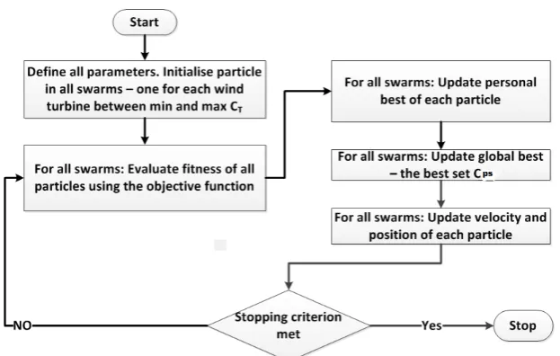
3.2. Particle Swarm Optimisation (PSO) 126
PSO consists of particles which move through the solution space in an organised way, by 127
developing a collective intelligence for solving complex optimisation problems [30]. An individual 128
particle represents a potential solution to the given problem. A swarm of particles represents a 129
dimension of the objective function / control problem. Every particle’s best fitness value estimated in 130
different iterations is recorded as the local best of that specific particle. All local bests are compared 131
with each other and the best fitness value is recorded as global best. Local and global bests along with 132
the particles’ current positions are used to estimate a velocity for finding the best possible solution 133
[31]. This is a repetitive process which terminates when a suitable solution is acquired or number 134
of iterations is exhausted. The number of swarms required for optimizing the objective function in 135
equation (5) is equal toN. Power production of each turbine is a dimension of the net farm production. 136
The value ofOFin equation (5) is minimised in such a way, that each turbine’s optimumCPorαis 137
Figure 1.PSO flowchart for solving coordinated control problem
4. Wind Farms Case Studies 139
The Brazos, SMV and Lillgrund wind farms are used as case studies in this work. These three 140
wind farms represent a diverse set in terms of layout, terrain and wind characteristics. A brief overview 141
of these wind farms case studies is given as follows. 142
4.1. Brazos 143
Turbines in the Brazos wind farm are installed in a non-grid shape with downwind spacing 144
up to 8Dand crosswind spacing of as low as 2D[7]. Each row in the Brazos can be assumed as a 145
sub-farm for faster and efficient optimisation. The encircled row in Figure2a is used as the case study 146
for optimisation in this work. Seven Mitsubishi MWT 1000 turbines are installed in this row with a 147
spacing of 3D[7]. This case study is referred to Brazos-row. Brazos has flat terrain with low grass [7]. 148
The wind-rose in Figure2b shows the wind characteristics on site based on data from year 2004 - 2006. 149
Figure 2.(a) Brazos layout (case study row encircled) (b) Wind-rose obtained with data from 2004-2006
4.2. Le Sole de Moulin Vieux (SMV) 150
Seven Senvion MM82 2050 kW wind turbines are installed in almost like a one-dimensional array 151
with a spacing of 3.3Dto 4.3Das depicted in Figure3a in the SMV wind farm. SMV has a rough terrain, 152
woods can cause abrupt changes in wind speed and direction [8]. Figure3b shows wind characteristics 154
in the farm. 155
Figure 3. (a)Layout of the SMV wind farm(b)Wind-rose obtained with data from 2011 - 2015
4.3. Lillgrund 156
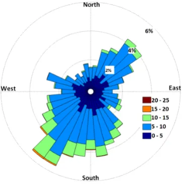
Lillgrund contains 48 Siemens SWT-2.3-93 turbines, installed in 8 rows as can be seen in Figure4a. 157
Downwind spacing is 4.5Dwhile crosswind spacing is 3.5D. Lillgrund is an offshore wind farm. The 158
wind-rose in Figure4b shows wind characteristics in the wind farm. Wind data of 15 years (2000-2015) 159
was used in Figure4b using [32] at 50m height. Performance of this wind farm is significantly affected 160
by wakes due to the dense layout [5]. 161
Figure 4. (a)Lillgrund layout and turbines in setj(b)wind-rose obtained with data from 2000-2015
5. Methodology for Calculating Efficiency 162
This section details the methodology for obtaining efficiencies of the three wind farms case studies. 163
Equation (7) [2] is used for estimating efficiencies (η) of Brazos-row and SMV. The denominator (Pmax) 164
is simply the maximum possible farm production for a given wind speed in no-wake conditions. The 165
numerator (Pactual) is the actual net production of the farm. 166
η= Pactual
Pmax (7)
ηLill= Nj 48
48
∑
i=1 Pi
∑
j Pj
(8)
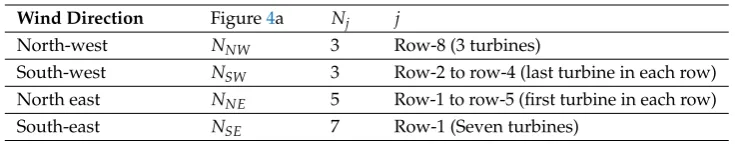
where average power of theithturbine is denoted by (Pi), (j) represents a set containing a specific 168
number of turbines (Nj) as per Table1. The number of turbines in setjis determined using free stream 169
wind direction. There can be four different combination in setjas it contains the turbines facing the 170
free-stream wind, as shown in Figure4a. Production of thejthturbine in setjis given by (Pj). 171
Table 1.Turbines in setj
Wind Direction Figure4a Nj j
North-west NNW 3 Row-8 (3 turbines)
South-west NSW 3 Row-2 to row-4 (last turbine in each row)
North east NNE 5 Row-1 to row-5 (first turbine in each row)
South-east NSE 7 Row-1 (Seven turbines)
6. Results and Analyses 172
Wake effects are negligible in above-rated conditions [5], hence only below-rated conditions are 173
assumed in the simulations in this section. Efficiencies based on WindPRO and real-time SCADA data 174
in full or near-full wake conditions are used as benchmarks. WindPRO direction bin is kept at 10◦, 175
which is the finest possible. WindPRO uses the standard onshore and offshore values ofkgiven in [34], 176
for wake estimation. TI-JM uses SCADA data for Brazos-row and SMV for tuning the initial value ofk 177
according to the conditions. For TI-JM and SCADA data, the directional resolution is maintained at 1◦. 178
TI-JM is first compared with SCADA data and WindPRO using efficiencies based on greedy control. 179
The optimal control strategies are then evaluated by comparing them with greedy control using TI-JM. 180
Contour plots of the three wind farms case studies in full-wake conditions are used for depicting a 181
comparison of conventional and coordinated control strategies. 182
Data filtering was applied to ensure that only operational turbines are analysed. It was observed 183
that the maximum efficiency in no-wake conditions for Brazos-row and SMV wind farms was not 100%. 184
Instead it was 82% for Brazos-row and 86% for SMV. These discrepancies may have been caused by 185
anomalies in SCADA data or other unknown operational issues. WindPRO and TI-JM do not consider 186
any anomalies or issues with data, taking only wake effects for wind deficit estimation. Therefore, 187
the maximum efficiency (82% for Brazos-row and 86% for SMV) is made 100% by simply adding the 188
difference (18% for Brazos-row, 14% for SMV) to efficiency at all points. This nullifies the impact of all 189
other issues by taking only the impact of wake effects on farms productions. The shifted efficiency 190
(based on SCADA data) can now be compared with efficiencies obtained with WindPRO and TI-JM. 191
Results and analyses for Brazos-row, SMV and Lillgrund wind farms are presented in sections6.1, 192
6.2and6.3respectively. These results are obtained using a basic computer (4 cores, 3.50GHz processor 193
and 16GB RAM). 194
6.1. Brazos-row 195
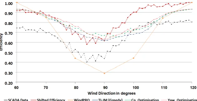
Efficiency of the Brazos-row is calculated using SCADA data from 2004–2006 provided by [35]. 196
The case study row is under wake effects in the directional sector of 90◦±30◦. Figure5depicts the 197
average efficiency in this directional sector. The sector 90◦±30◦can be further divided into bins as 198
follows. 199
• Full wakes (worst case) = 90◦±10◦ 200
The shifted efficiency in Figure5shows that efficiency can drop to as low as 58% in full-wake 202
conditions. WindPRO and TI-JM estimate that efficiency can be as low as 30% and 62% in full-wake 203
conditions. The standard Jensen model available in WindPRO is used with a constantk=0.07, for 204
such onshore terrain. WindPRO uses the WAsP model [17] for analysing the impact of terrain on 205
wake effects. On the other hand, TI-JM does not use any terrain model, rather it varieskaccording to 206
wind conditions, instead of keeping it constant as discussed in section2. TI-JM usedkup to 0.25 for 207
estimating wind speed deficits inside the farm. The initial value ofkis the standardkfor such terrains. 208
Wind direction is derived from the data obtained from met mast. 209
Figure 5.Brazos efficiency in 60◦−120◦directional sector
It can be seen in Figure5that WindPRO and TI-JM predict almost symmetrical efficiencies 210
around 90◦as it is a straight line (row) of turbines (Figure2a). However, the shifted efficiencies is 211
not symmetrical on both sides of 90◦. The efficiency predicted by TI-JM fits well with the shifted 212
efficiency in the 60◦−90◦sector. However, the efficiency is not that accurate in the 91◦−120◦sector. 213
Overall, TI-JM predicts better than WindPRO in most of the cases. TI-JM and WindPRO ignore 214
wake-meandering and wind shear effects, which can result in uncertainty in models’ prediction 215
accuracy. 216
BothCPand yaw-based optimised strategies can increase the average efficiency by up to 6% as 217
compared to greedy control as can be seen in Figures5and6. It was observed that coordinated control 218
based onCpoptimisation performed better in full or near-full wake conditions. Yaw optimisation can 219
produce better results in partial wake conditions. 220
The reduction inCPof upstream turbines depends upon wind speed and direction. Optimised 221
reduction inCPof the upstream turbines for curtailing their power production ranges between 3% 222
and 20%. In higher wind speeds, theCPcurtailment is minimal as wake effects are also minimal. 223
This is true for all the three wind farms case studies. In full-wake conditions, significantly larger 224
yaw-offset (up to±30◦) is required for deflecting the wake away from swept area of the wake affected 225
turbines. This converts a full-wake into partial wake for the downstream turbines but at the same 226
time significantly reduces production of the yawed turbine. A partial wake is converted into minimal 227
or no-wake situation using a yaw-offset in a range of±15◦, producing a significant increase in wake 228
affected turbines’ productions. The impact of this yaw-offset on the yawed turbine is considerably low, 229
Figure 6.Impact (% increase) of optimised control strategies on Brazos-row efficiency, relative to greedy control
Wind flow with state of the art greedy control, CP and yaw-based optimised strategies in 231
full-wake conditions is shown in Figure 7. The lower wind speed deficit inside the wind farm 232
withCPoptimisation, as compared to greedy control can also be seen. Figure7c depicts the wake 233
skewing from the downstream turbines. The wake-added turbulence intensity increasesk, hence the 234
wake spread inside the farm as shown in Figures7. The optimisation process (in a single simulation) 235
took less than 15 seconds for Brazos-row. 236
Figure 7. Comparison of control strategies for Brazos-row at 8m/s in full wakes. Range ofkvaries from 0.07 (free-stream) to 0.025 (deep inside the farm)(a)conventional greedy control(b)Optimised control based onCP(c)Optimised control based on yaw-offset
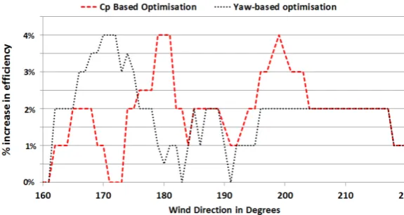
6.2. Le Sole de Moulin Vieux (SMV) 237
SCADA data of the SMV wind farm from 2011–2014 is provided by Maïa Eolis (now Engie Green). 238
Full or near-full wake conditions are assumed in the simulations. Average efficiency from the south 239
160◦−220◦is shown in Figure8. The sector 160◦−220◦is chosen because of the prevailing wind 240
direction and significant wake effects observed in these directions. Analyses of the SCADA data show 241
that shifted efficiency can drop to 78% in the worst conditions. WindPRO (standard Jensen model with 242
k=0.07 and WAsP) predicted that efficiency can be as low as 70% with such layout and terrain. TI-JM 243
estimated a minimum efficiency of 76% in the worst case. It was observed thatkcan increase up to 244
Figure 8.SMV Efficiency in 160◦−220◦sector
It can be observed in Figure8that TI-JM matches the shifted efficiency better in 160◦−200◦, while 246
WindPRO produces better results in 200◦−220◦. TI-JM under-estimates wake losses in the 200◦−220◦ 247
sector, concluding that thekneeds to be further increased in this sector for better wake estimation. 248
Wind conditions on site due to the nearby woods (section4.2) also adds to the complexity for wind 249
deficit prediction. 250
It can be observed in Figures8and9that optimised control strategies can increase efficiency 251
by up to 4%. The directional sector 160◦−220◦ cannot be divided into partial and full wakes for 252
the whole wind farm in this case. Turbines in the SMV are not installed in a complete straight line 253
(Figure3a), hence these turbines will be under different wake conditions for a given wind direction [8]. 254
SMV5 produces full wakes on SMV1-SMV4 in 180◦±10◦. For the same wind direction, SMV5 is under 255
minimal wake effects of SMV6 and SMV6 is under negligible wake effects of SMV7. SMV6 experiences 256
significant wake effects of SMV7 in 200◦±10◦but at the same time all other turbines experiences 257
minimal wake effects from their corresponding upstream turbines. The optimised yaw-offsets andCP 258
curtailment settings were the same as for Brazos-row (section6.1). 259
Figure 9. Impact (% increase) of optimised control strategies on SMV efficiency, relative to greedy control
A comparison of wind flow using conventional and optimised control strategies is shown in 260
Figure 10.Comparison of control strategies for SMV at 8m/s from north. Range ofkvaries from 0.07 (free-stream) to 0.020 (deep inside the farm)(a)conventional greedy control(b)Optimised control based onCP(c)Optimised control based on yaw-offset
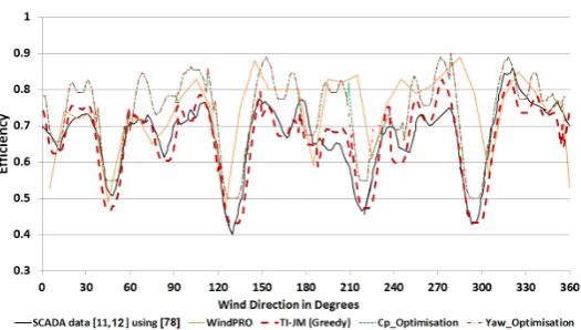
6.3. Lillgrund 262
Lillgrund efficiency can be as low as 40% in the worst case, when turbines are under full wake 263
effects [5]. Due to the dense layout of the farm, turbines experience wake effects in almost all wind 264
directions. Therefore, the 360◦ farm efficiency curve available in [5] was digitised using [36] and 265
reproduced in Figure 11. Other details such as farm layout, surface roughness length, turbine 266
characteristics and turbulence intensity were provided by [33]. As per [33], the value of kshall 267
be tuned for best fit as required by the wake model. It was noted in the simulations that values of 268
kin equation (9) provide the best fit (for TI-JM) with actual efficiency. WindPRO used the standard 269
k=0.04 for offshore wind conditions in this case. Though WindPRO captures shape of the efficiency 270
curve, yet in most of the cases, it underestimates wake effects. On the other hand, TI-JM predicts wake 271
effects with almost 95% accuracy in this case. 272
k=0.04 i f u0≤7.0m/s
k=0.08 i f 7.0m/s<u0≤12.0m/s wind speeds>12not considered as suggested in[5]
(9)
Figure 11.Average 360◦efficiency of Lillgrund in below-rated conditions
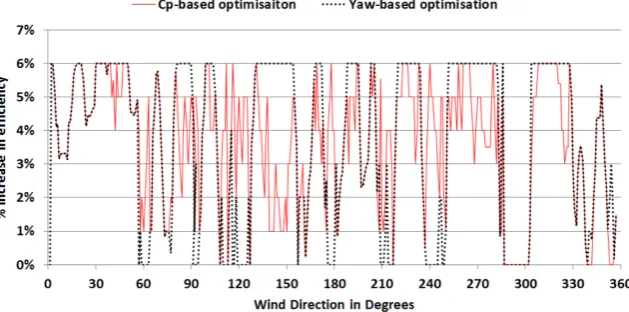
Dense wind farms such as Lillgrund can significantly benefit from coordinated control. Full 273
directions. It can be seen in Figure12that efficiency can be improved by a maximum of 6% with 275
optimised control strategies. It can also be observed in Figure12that efficiency can be increased in 276
almost all wind directions as wake effects are always present in the farm. In partial wakes, yaw-based 277
optimisation provides a better opportunity for efficiency improvement whileCPoptimisation is more 278
suitable in full-wake conditions. This observation is same as for Brazos-row. The ranges forCP 279
curtailment and yaw-offsets are same as Brazos-row and SMV. 280
Figure 12.Impact (% increase) of optimised control strategies on Lillgrund efficiency, relative to greedy control
A comparison of wind flow using conventional and optimised control strategies is shown in 281
Figure13. The optimisation process (in a single simulation) took less than 50 seconds for Lillgrund. 282
Figure 13. Comparison of control strategies for Lillgrund at 8m/s in full-wake conditions. Range ofkvaries from 0.04 (free-stream) to 0.14 (deep inside the farm).(a)conventional greedy control(b) Optimised control based onCP(c)Optimised control based on yaw-offset
7. Conclusion 283
Wake-effects can have a significant impact on economic performance of wind farms by increasing 284
production losses and fatigue loads. This work presented an intelligent and fast processing farm 285
controller for reducing wake effects. Optimised coordinated control strategies are used for increasing 286
farm production by optimally varyingCPor yaw-angles. The optimised control strategies uses TI-JM 287
for estimating wind speeds inside the wind farms and PSO for optimisation. TI-JM is an improved 288
version of the standard Jensen model. TI-JM takes deep array effect into consideration using wake 289
added turbulence intensity for estimatingk. It can accurately predict wind speed inside a wind farm 290
in most of the cases for the wind farms case studies, hence farm production and efficiency. Both the 291
CP-based and yaw-based optimised strategies increased wind farm efficiency as compared to the 292
conventional greedy control. The system has been designed for all wind conditions, however it is 293
tested only for static wind conditions using TI-JM. Simulations confirm that average efficiency can be 294
increased by up to 6% for Brazos-row and Lillgrund while 4% for SMV. SMV and Brazos-row were 295
optimised in a maximum of 15 seconds while Lillgrund always took less than 50 seconds, using a basic 296
computer. It is concluded thatCPoptimisation is suitable in full-wake conditions for net production 297
maximisation. Yaw-optimisation is beneficial for farm production maximisation in partial-wake 298
conditions. As a future work, these results shall be validated using high fidelity wake models. It shall 299
is only to analyse production maximisation. Fatigue load optimisation would require a multi-objective 301
optimisation for minimising loads and maximising production of the farm, which is left for future 302
work. Furthermore, a wind turbine has a designed service life of almost 20 to 25 years, however due to 303
the technological advances and ever-growing size of turbines, farm operators replace these turbines 304
much earlier than their end of life. Hence, the increase in fatigue loading for some gain in production 305
might be economically beneficial. This can be further investigated in the future.Author Contributions: 306
This work is primarily based on the PhD research work of Tanvir Ahmad at Durham University, UK. This PhD 307
work was supervised by Peter C. Matthews and Behzad Kazemtabrizi. Abdul Basit and Samia Akhtar provided 308
support in the data analyses section. Juveria Anwar helped in visualization of some of the results. Olivier Coupiac 309
provided assistance in using WindPRO and obtaining data for the Lillgrund wind farm. 310
Funding:The PhD research was funded by the Commonwealth Scholarship Commission (CSC), UK (reference: 311
PKCS-2013-384). Pakistan Council of Renewable Energy Technologies (PCRET) funded this publication jointly 312
with the US Pakistan Center for Advanced Studies in Energy, University of Engineering & Technology Peshawar, 313
Pakistan. 314
Conflicts of Interest:“The authors declare no conflict of interest.” 315
Abbreviations 316
The following abbreviations are used in this manuscript: 317
PSO Particle Swarm Optimisation
TI-JM Turbulence Intensity based Jensen Model
SMV Le Sole de Moulin Vieux 318
319
1. Bitar, E.; Seiler, P. Coordinated control of a wind turbine array for power maximization. American Control 320
Conference (ACC). IEEE, 2013, pp. 2898–2904. 321
2. Pao, L.Y.; Johnson, K.E. A tutorial on the dynamics and control of wind turbines and wind farms. American 322
Control Conference, ACC’09; IEEE: 172, 2009; pp. 2076–2089. 323
3. Johnson, K.E.; Thomas, N. Wind farm control: addressing the aerodynamic interaction among wind 324
turbines. American Control Conference, ACC’09; IEEE: 155, 2009; pp. 2104–2109. 325
4. Ahmad, T.; Girard, N.; Kazemtabrizi, B.; Matthews, P. Analysis of two onshore wind farms with a dynamic 326
farm controller. EWEA, Paris France, 2015. 327
5. Dahlberg, J.A. Assessment of the Lillgrund windfarm: Power performance. Technical Report 21858-1, 328
Vatenfall, Vindkraft AB, 2009. 329
6. Aranda, F.A. Wind Farm Control Methods, IEA R&D Wind Task 11 - Topical Expert Meeting. Technical 330
report, International Energy Agency, 2012. 331
7. Ahmad, T. Wind Farm Coordinated Control and Optimisation. PhD thesis, School of 332
Engineering & Computing Sciences, Durham University UK, 2017. Availalble online at 333
[http://etheses.dur.ac.uk/12323/1/Tanvir_Thesis_Final_Submission.pdf]. 334
8. Ahmad, T.; Coupiac, O.; Pettit, A.; Guignard, S.; Girard, N.; Kazemtabrizi, B.; Matthews, P. Field 335
Implementation and Trial of Coordinated Control of Wind Farms.IEEE Transactions on Sustainable Energy 336
2017. 337
9. Ambekar, A.; Ryali, V.; Tiwari, A.K. Methods and systems for optimizing farm-level metrics in a wind 338
farm, 2015. US Patent 9,201,410. 339
10. Soleimanzadeh, M.; Wisniewski, R.; Kanev, S. An optimization framework for load and power distribution 340
in wind farms. Journal of Wind Engineering and Industrial Aerodynamics2012,107, 256–262. 341
11. Jensen, N.O. A note on wind generator interaction. Technical Report Risø -M-2411, Risø National 342
Laboratory, Roskilde, Denmark, 1983. 343
12. Katic, I.; Højstrup, J.; Jensen, N.O. A simple model for cluster efficiency. European Wind Energy Association 344
Conference and Exhibition, 1986, pp. 407–410. 345
13. Park, J.; Kwon, S.; Law, K.H. Wind farm power maximization based on a cooperative static game approach. 346
SPIE Smart Structures and Materials+ Nondestructive Evaluation and Health Monitoring. International 347
14. Ahmad, T.; Matthews, P.; Kazemtabrizi, B. PSO Based Wind Farm Controller. The 11th edition of 349
the International Conference on Evolutionary and Deterministic Methods for Design, Optimization and 350
Control with Applications to Industrial and Societal Problems, EUROGEN-2015 Glasgow, UK, 2015, pp. 351
277–283. 352
15. González, J.S.; Payán, M.B.; Santos, J.R.; Rodríguez, Á.G.G. Maximizing the overall production of wind 353
farms by setting the individual operating point of wind turbines. Renewable Energy2015,80, 219–229. 354
16. Marden, J.R.; Ruben, S.D.; Pao, L.Y. Surveying game theoretic approaches for wind farm optimization. 355
Proceedings of the AIAA aerospace sciences meeting, 2012, pp. 1–10. 356
17. Nielsen, P.; Villadsen, J.; Kobberup, J.; Madsen, P.; Jacobsen, T.; Thøgersen, M.L.; Sørensen, M.V.; Sørensen, 357
T.; Svenningsen, L.; Motta, M.; Bredelle, K.; Funk, R.; Chun, S.; Ritter, P.WindPRO 2.7 User Guide. EMD 358
International A/S, Aalborg, Denmark, 3rd ed., 2010. 359
18. Annoni, J.; Gebraad, P.M.; Scholbrock, A.K.; Fleming, P.A.; van Wingerden, J.W. Analysis of 360
axial-induction-based wind plant control using an engineering and a high-order wind plant model. Wind 361
Energy2015,19, 1135–1150. 362
19. Knudsen, T.; Bak, T.; Svenstrup, M. Survey of wind farm control power and fatigue optimization.Wind 363
Energy2014. 364
20. Qian, G.W.; Ishihara, T. A New Analytical Wake Model for Yawed Wind Turbines.Energies2018,11, 665. 365
21. Marathe, N.; Swift, A.; Hirth, B.; Walker, R.; Schroeder, J. Characterizing power performance and wake of 366
a wind turbine under yaw and blade pitch. Wind Energy2016,19, 963–978. 367
22. Wan, S.; Cheng, L.; Sheng, X. Effects of yaw error on wind turbine running characteristics based on the 368
equivalent wind speed model. Energies2015,8, 6286–6301. 369
23. Park, J.; Law, K.H. A data-driven, cooperative wind farm control to maximize the total power production. 370
Applied Energy2016,165, 151–165. 371
24. Boorsma, K. Power and loads for wind turbines in yawed conditions. Technical report, ECN-E-12-047, 372
ECN, Petten, The Netherlands, 2012. 373
25. Annoni, J.; Fleming, P.; Scholbrock, A.; Roadman, J.; Dana, S.; Adcock, C.; Porte-Agel, F.; Raach, S.; 374
Haizmann, F.; Schlipf, D. Analysis of Control-Oriented Wake Modeling Tools Using Lidar Field Results. 375
26. Wagenaar, J.; Machielse, L.; Schepers, J. Controlling wind in ECN scaled wind farm. Proc. Europe Premier 376
Wind Energy Event2012, pp. 685–694. 377
27. Corten, G.; Schaak, P.; Bot, E. More power and less loads in wind farms: Heat and Flux. European Wind 378
Energy Conference & Exhibition, London, UK, 2004. 379
28. Schram, C.; Vyas, P. Windpark turbine control system and method for wind condition estimation and 380
performance optimization, 2005. US Patent App. 11/288,081. 381
29. Kanev, S.; Savenije, F. Active Wake Control: loads trends. Technical Report ECN-E–15-004, ECN, Petten, 382
The Netherlands, 2015. 383
30. Kennedy, J.; Spears, W.M. Matching algorithms to problems: an experimental test of the particle swarm 384
and some genetic algorithms on the multimodal problem generator. Proceedings of the IEEE international 385
conference on evolutionary computation. Citeseer, 1998, pp. 78–83. 386
31. Kennedy, J.; Eberhart, R. Particle swarm optimization. Proceedings of IEEE international conference on 387
neural networks; Perth, Australia: 162, 1995; Vol. 4, pp. 1942–1948. 388
32. Rienecker, M.M.; Suarez, M.J.; Gelaro, R.; Todling, R.; Bacmeister, J.; Liu, E.; Bosilovich, M.G.; Schubert, 389
S.D.; Takacs, L.; Kim, G.K.; others. MERRA: NASA’s modern-era retrospective analysis for research and 390
applications. Journal of Climate2011,24, 3624–3648. 391
33. Moriarty, P.; Rodrigo, J.S.; Gancarski, P.; Chuchfield, M.; Naughton, J.W.; Hansen, K.S.; Machefaux, E.; 392
Maguire, E.; Castellani, F.; Terzi, L.; others. IEA-Task 31 WAKEBENCH: Towards a protocol for wind 393
farm flow model evaluation. Part 2: Wind farm wake models. Journal of Physics: Conference Series. IOP 394
Publishing, 2014, Vol. 524, p. 012185. 395
34. Thørgersen, M.; Sørensen, T.; Nielsen, P.; Grötzner, A.; Chun, S.WindPRO/PARK: Introduction to wind turbine 396
wake modelling and wake generated turbulence. EMD International A/S, Niels Jernesvej 10, 9220 Aalborg, 397
2005. Available at: http://www.emd.dk/files/windpro/manuals/for_print/Appendices-all_UK.pdf. 398
35. Bueno Gayo, J. ReliaWind Project Final Report. Technical Report Project Nr 212966, Gamesa Innovation 399
and Technology, 2011. 400