doi: 10.3389/fmech.2019.00035
Edited by: Michael John Gollner, University of Maryland, College Park, United States
Reviewed by: Shiyou Yang, Ford Motor Company, United States Xinyan Huang, Hong Kong Polytechnic University, Hong Kong Eric Link, National Institute of Standards and Technology (NIST), United States
*Correspondence: Khalid Moinuddin [email protected]
Specialty section: This article was submitted to Thermal and Mass Transport, a section of the journal Frontiers in Mechanical Engineering
Received:29 January 2019 Accepted:31 May 2019 Published:28 June 2019
Citation: Khan N, Sutherland D, Wadhwani R and Moinuddin K (2019) Physics-Based Simulation of Heat Load on Structures for Improving Construction Standards for Bushfire Prone Areas. Front. Mech. Eng. 5:35. doi: 10.3389/fmech.2019.00035
Physics-Based Simulation of Heat
Load on Structures for Improving
Construction Standards for Bushfire
Prone Areas
Nazmul Khan1,2, Duncan Sutherland1,2,3, Rahul Wadhwani1,2and Khalid Moinuddin1,2*
1Institute for Sustainable and Livable Cities, Victoria University, Melbourne, VIC, Australia,2Bushfire and Natural Hazards Cooperative Research Centre, Melbourne, VIC, Australia,3School of Science, University of New South Wales, Canberra, ACT, Australia
Australian building standard AS 3959 provides mandatory requirements for the construction of buildings in bushfire prone areas in order to improve the resilience of the building to radiant heat, flame contact, burning embers, and a combination of these three bushfire attack forms. The construction requirements are standardized based on the bushfire attack level (BAL). BAL is based on empirical models which account for radiation heat load on structure. The prediction of the heat load on structure is a challenging task due to many influencing factors: weather conditions, moisture content, vegetation types, and fuel loads. Moreover, the fire characteristics change dramatically with wind velocity leading to buoyancy or wind dominated fires that have different dominant heat transfer processes driving the propagation of the fire. The AS 3959 standard is developed with respect to a quasi-steady state model for bushfire propagation assuming a long straight line fire. The fundamental assumptions of the standard are not always valid in a bushfire propagation. In this study, physics based large-eddy simulations were conducted to estimate the heat load on a model structure. The simulation results are compared to the AS 3959 model; there is agreement between the model and the simulation, however, due to computational restrictions the simulations were conducted in a much narrower domain. Further simulations were conducted where wind velocity, fuel load, and relative humidity are varied independently and the simulated radiant heat flux upon the structure was found to be significantly greater than predicted by the AS 3959 model. The effect of the mode of fire propagation, either buoyancy-driven or wind dominated fires, is also investigated. For buoyancy dominated fires the radiation heat load on the structure is enhanced compared to the wind dominated fires. Finally, the potential of using physics based simulation to evaluate individual designs is discussed.
1. INTRODUCTION
Bushfire or wildfire is an integral part of the Australia environment and costs millions of dollars every year in terms of losses to the economy. The infamousBlack Saturdaybushfire of 2009 alone had an estimated economic cost of AUD 4.4 billion and destroyed ∼3,500 structures (McLeod et al., 2010;
Ronchi et al., 2017). Previously, the 2003 Canberra fire (Blanchi and Leonard, 2005) destroyed roughly 390 houses and cost an estimated AUD 0.35 billion in losses. Over the past decade, the frequency of bushfire around the world has increased (Jolly et al., 2015).Ronchi et al.reported some of the economic costs of wildfire in North America to be between 0.4 and 7 billion USD in the last decade. The size of fires is also increasing. Recently, large and devastating bushfires, termed mega bushfire or mega wildfire, have emerged. Wildfires are classified as mega wildfires if the fire occurs at large spatial scale coupled with strong wind reaching up to 100 km/h, firestorm events and massive ember generation can cause massive evacuation, devastation, and loss of life. These fires are dynamic and difficult to manage (Mell et al., 2010). Dynamic bushfire behavior is also present in smaller bushfires. Empirically-based operational fire models struggle to account for extreme and dynamic bushfire behavior and existing operational fire model show significant difference in predicting the bushfire propagation (Cruz and Alexander, 2013). Some of the recent “mega wildfires” are the 2016 Fort McMurray fire, Canada; the 2017 Californian wildfires, USA; the 2017 Portugal wildfires, Portugal (Ronchi et al., 2017). The effect of these bushfires is not limited to economical damages, the fires also cause massive evacuation of communities and present challenges to emergency personnel. The Black Saturday fire, Australia, caused 7500 people to evacuate (McLeod et al., 2010). Many people, who did not evacuate early, died during their attempted late evacuation. The high number (173) of fatalities in 2009 Black Saturday fire is one such identified bushfire case where late evacuation resulted in the loss of life (McLeod et al., 2010; Whittaker et al., 2013). Expansion of suburban areas into previously undeveloped forest and grassland also increases the impact of fires on the population. As the populations of major cities grows, so does the area of residential areas bordering fire prone bushland. City planners and building authorities must therefore plan new developments to be resilient to the risks of bushfires.
1.1. Building in Bushfire Prone Areas
A recent study in the US (Radeloff et al., 2018) showed that there is a significant increase in the wildland-urban-interface (WUI), WUI houses, and people living in WUI from 1990-2010. One definition of the WUI (Radeloff et al., 2005) is as an area in which:
• There are at least 6.17 housing units/km2with vegetation area of more than 50% of terrestrial area, or
Abbreviations:FDI, Fire Danger Index; GFDI, Grass Fire Danger Index; RoS, Rate-of-spread (of a fire); BAL, Bushfire attack level.
• There are more than 6.17 housing unit/km2 with vegetation
area less than 50% of terrestrial area and is less than 2.4 km away from vegetation which has an area of greater than 5 km2 and have vegetation area of greater than 75%.
These definitions depend somewhat on the jurisdiction. In Australia, bushfire prone areas (BPA) are classified by Australian Standard 3959 (AS 3959, 2009). The BPA is classified into three classes:
• Bushfire hazard level 2 (BHL2): Areas of forest, woodlands, scrub, shrublands, mallee, and rainforest where there is potential for bushfire behavior such as a crown fire, extreme levels of radiant heat, and extreme ember attack. BHL2 does not include grasslands. An area of BHL2 that is larger than 4 hectares will be mapped as BPA including a buffer of 300 m.
• Bushfire hazard level 1 (BHL1): Areas of forest, woodlands, scrub, shrublands, mallee, rainforest, and unmanaged grasslands where there is potential for bushfire behavior such as crown fire, grassfire, and ember attack. An area of BHL1 that is between 2 and 4 hectares that is not unmanaged grassland will be mapped as BPA including a buffer of 150 m. An area of unmanaged grassland larger than 2 hectares will be mapped as BPA including a buffer of 60 m.
• Bushfire hazard level low (BHL low): Areas where extent of bushfire attack is very low e.g., managed grassland park, airports, or botanical gardens.
Australian standard 3959 (AS 3959, 2009) was developed to specify the necessary design for the structures located at BPA. The intention of AS 3959 was improving the resilience of buildings against the bushfire attack (radiant heat, direct flame contact, burning ember, or a combination of these three factors) to mitigate the risk of bushfire through better adaptability of structures situated in the WUI. While the topic of this paper is limited to AS 3959, the US standard developed by National Fire Protection Association (NFPA). NFPA 1144 (NFPA 1144, 2013) uses a similar model to prescribe design requirements for structures in the WUI areas of the US. There are several drawbacks of AS 3959 that have previously been reported (Roberts et al., 2017; Sharples, 2017). A particular limitation of AS 3959 is the lack of quantified ember loading during a fire event. Embers are the leading cause of house loss; in the Canberra 2003 fires, 229 houses were destroyed in the suburb of Duffy and 106 of the houses were ignited by embers alone (Blanchi and Leonard, 2005). AS 3959 only provides a small amount of guidance about ember attack increasing with fire danger. AS 3959 is based upon an empirical model for radiation heat load upon the structure. The model and its limitations will now be discussed.
1.2. Empirical Models and FDI
under the weather and fuel conditions. The McArthur Forest fire danger index FDI has a reference value set to 100 for the 1939 Black Fridaybushfire (McArthur, 1967). There are many instances where this reference value was breached, for example, theBlack Saturdaybushfire of 2009, where FDI value for forest was more than 172 and 241 for grass lands (Tollhurst, 2009). In the state of New South Wales, Australia, FDI of above 100 suggests that structures will not survive and hence evacuation of occupants is required. There are several versions of the fire danger index for different fuel types and for different fire spread models and all FDI are based on the same principles. Given that this work focus on grassland fuels, the relevant fire danger index is the grassland fire danger index (GFDI):
GFDI=
3.35wexp(−0.097mc+0.0403u) mc≤18.8%, 0.299wexp(−1.686mc+0.0403u)(30−mc)
18.8%<mc<30%.
(1)
wherewis the fuel weight (T/Ha),mcis fuel moisture content as
a percentage, anduis the wind speed at 10 m high in km/h. The moisture content is modeled by the following correlation
mc= 97.7+4.06RH
T+6 −0.00854RH+ 3000
C −30, (2)
whereRHis relative humidity (%),Tis ambient temperature (◦C)
is the curing index (0−100%), a measure of the amount of dead
material in the grassland. TheGFDIis used to determine the rate of spread of the fireRoS, which is used to model the intensity of the fire. TheRoSis
RoS=0.13GFDI. (3) The fire intensity model for grassland [AS 3959 fuel class G, and also class C (shrubland), D (scrub), and E (Mallee/Mulga)] is given by Byram’s model:
I= H w RoS
36 , (4)
whereHis heat of combustion (in the Byram modelH = 18.6 MJ/kg) and flame lengthLf is subsequently calculated using
Lf =0.0775I0.46, (5)
and flame height may be determined using:
Fh=Lfcosα, (6)
whereαis the angle between the ground surface and the flame height which is not subsequently modeled. An algorithm in AS 3959 is provided to compute the flame angle which gives the maximum view factor between the flame and the structure to provide an estimate of heat load in the worst-case scenario. On a flat ground the view factor will be maximized atα = π/2. The lack of a model ofα is a limitation of the standard, especially since some limited flame angle correlations, for exampleWeise and Biging (1996), do exist in the literature. To calculate emitted radiant heat flux, an estimated flame temperature (1090 K) is used
instead of fire intensity; note that intensity does determine the flame length.
The emitted radiant heat flux is computed from the flame temperature, flame height, and flame width. Here flame width refers to the length of the fire front taken as arbitrarily as 100 m in the AS 3959 standard. These fire behavior parameters are used to compute the emitted radiant heat flux load available from the fire present in the particular vegetation. The radiant heat emitted by the flame is
qr,emitted=LfcosαFwσ ǫTf4, (7)
whereTfis the flame temperature (K),σis the Stefan-Boltzmann
constant (5.67−8W/m2K4),ǫis called emissivity and represents
the non-ideal blackbody characteristics of the material.ǫis taken as the value for soot (0.9).Fwis the flame width.
AS 3959 assumes a constant value of flame temperature of 1090 K however the instantaneous value of flame temperature can be higher than 1200 K (Worden et al., 1997). It can be seen from Equation (7) that the thermal radiation is proportional to the fourth power of the flame temperature and directly proportional to effective area of the flame. Because the flame temperature is raised to the fourth power and so any errors in flame temperature lead to much larger errors in emitted radiant heat flux. The radiant heat flux received at the structure depends on two more parameters: the view factorF1,2, which represents
the effective solid angle between the flame in the classified vegetation and structure, andφ, the atmospheric transmissivity to account for how much radiative heat is absorbed before reaching the structure. These two parameters are combined with the calculation of heat flux load at the site to estimate effective radiant heat flux at the structure. That is,
qr,effective=LfcosαFwF1,2φσ ǫTf4. (8)
AS 3959 (table 3.1) classifies the bushfire attack level (BAL) into six categories based on the radiant heat flux qr,effective at the
structure
• BAL- LOW: considered safe situation for heat flux less 12.5 kW/m2and no ember attack. Hence, no special construction requirements.
• BAL- 12.5, 19, 29, 40: special construction is required, the numbers correspond to heat fluxes of 12.5, 19, 29, and 40 kWm−2, respectively. These cases involve ember attack
however there is no quantification of ember attack, only that ember attach is suggested to increase with the heat flux.
• BAL- FZ: are considered situations in which direct flame contact in addition to heat flux more than 40 kWm−2 and
ember showers are expected to the structure.
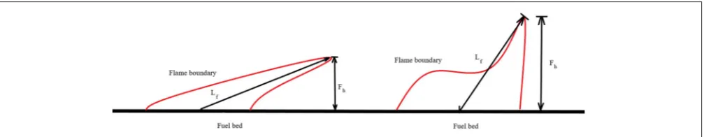
3959 radiation model in certain situations and generally in mega-bushfire might severely under predict radiation heat flux load. In the 2017 Iberian wildfires, Portugal, social media posts showed that many of the structure were exposed to multiple fire fronts showing a higher heat flux exposure on the structure (Viegas, 2017). The other aspect that radiant heat flux depends upon is view factor. The dynamic nature of a fire front changes the structure of flame hence affecting the view factor. The view factor can also change significantly due to different topography that is, if the fire is progressing down a slope toward the structure would have higher view factor than a fire progressing up the slope toward the structure. AS 3959 does include the topography in the computation of the view factor. Because we are only considering flat ground for this study, we omit discussion of the slope corrections to view factor. Another potential limitation of the AS 3959 approach is the lack of consideration of any flame geometry. The lack of a flame angle model may also be a critical flaw; it has been established for some time that there are two modes of fire propagation in wild, industrial, and building fires (Apte et al., 1991; Morvan and Frangieh, 2018). Grassfires have been characterized as wind dominated and buoyancy dominated fires (Dold and Zinoviev, 2009; Moinuddin et al., 2018; Morvan and Frangieh, 2018). In the wind dominated mode the shearing fluid flow (that is, the wind) dominates over the buoyant flow (the updraft from the fire plume). The flame is elongated and confined to a boundary layer structure,Figure 1A. In the buoyancy dominated mode, the updraft from the fire is sufficient to overcome the shearing forces of the driving wind and the flame becomes more vertical, see Figure 1B. In the wind dominated mode, the flame height is low and so the view factor will be small compared to the buoyancy dominated mode, however, because the fire plume is confined to a boundary layer there will be a high convective heat flux downstream of the fire. In the buoyancy dominated mode the plume is vertical and therefore the convective heat flux ahead of the fire will be small compared to the wind dominated mode. However, because the flame is vertical, the radiant heat flux ahead of the fire will be high compared to the wind dominated mode. For a realistic parameter range, wind dominated fires will have highGFDI(Equation 1) because of the exponential growth with wind speed. As a fire transitions from a buoyancy dominated fire to a wind dominated fire due to an increase in wind speed theGFDIwill increase. The fire intensity is expected to increase due to the increase inGFDI
andRoS(Equation 3). The AS 3959 model (Equation 5) predicts monotonic increase in flame height with increasing RoS and therefore, assuming flat ground, increased radiation load upon a structure. However, we hypothesize that if the fire becomes wind dominated the flame height will decrease and the corresponding increase in intensity may not be sufficient to ensure that the heat load on the structure increases with increasing wind speed.
The Byram convective number,Ncis used to quantify if a fire is
buoyancy dominated or wind dominated (Morvan and Frangieh, 2018). The Bryam number is defined by
Nc= 2gI
CpρTa(u10−RoS)3
, (9)
whereg = 9.8 ms−2 is the gravitation acceleration constant,
Tais the ambient temperature,Ta = 305 K in the simulations
presented here, the densityρ = 1.2 kg/m3 and specific heat of airCp = 1.0 kJ/kg K.u10 is the driving wind speed at 10 m
high.u10 is a chosen because wind speed measured at 10 m is
a meteorological standard. The factor of two in the definition of Nc is merely conventional. Fires are conclusively buoyancy
dominated ifNc≥10, wind dominated ifNc≤2, and ambiguous if 2<Nc<10.
1.3. Present Study
In this work we conduct simulations to compare the radiation heat load upon a structure, as close as computationally possible, from the fire scenario in AS 3959 predicted by the BAL set out in the standard, to the radiation heat load simulated by a physics based model. The idea is to assess the validity of the standard as it stands, rather than looking to extend the standard to include new features such as ember attack. Specifically, we will
1. identify if the BAL classification values are supported by physics-based simulation,
2. assess the sensitivity of the radiation heat load to the wind speed, fuel load, and relative humidity,
3. and examine the differences in heat load on a structure between buoyancy dominated fires and wind dominated fires.
The simulations are as close to the AS 3959 standard as computationally practical. However, due to computational restrictions the fire width is considerably reduced from 100 to 20 m. However, if the radiative heat load predicted by a 20 m wide fire is larger than predicted by AS 3959, it is reasonable to assume that the 100 m wide fire will exceed the standard by a larger amount. For simplicity we consider a grassland fuel atGFDI=50 to match the fuel classG in AS 3959. Further simulations are conducted to assess the effect of varying the driving wind speed and fuel load on the heat flux received by a structure and to determine if the different modes (wind dominated or buoyancy dominated) fire propagation effects the radiative heat load upon a structure. This work is intended to provide an introductory framework for the use of physics-based models in construction standards for properties in bushfire prone areas.
2. PHYSICS BASED SIMULATION
2.1. Fire Dynamics Simulator (FDS)
and structure of the grass, which exerts an aerodynamic drag force, is also represented as a momentum sink in the Navier-Stokes equations. Conduction within the solid fuel is modeled, but the contribution of conduction to the overall heat transfer is negligible. The convective heat transfer from the flame to the fuel bed is modeled using an empirical correlation for convective heat transfer to vertical circular cylinders. Radiation heat transfer is approximated by solving the radiation transport equation using a discrete ordinates method. A problem arises with this approach; because the combustion zone is difficult to resolve with LES the gas temperature can be under predicted in the flame. Because radiation depends on the fourth power of flame temperature, care is required so that unacceptable errors in radiative heat flux do not occur. The source of radiation is modeled by a piecewise function for the flaming and non-flaming regions. Outside the flaming zone, whereTis well resolved and there is no difficulty. Inside the flaming zone the radiation source is a function of the local heat release per unit volume.
FDS uses a fast chemistry model of combustion and where the mixture fraction of fuel and air is higher than the stoichiometric value, the fuel is considered burnt. See Mell et al. (2007), Mell et al. (2009), and McGrattan et al. (2013b) for a full and careful discussion of the physics-based model and the numerical methods used. FDS has been carefully validated for the simulation of grassfires. BothMell et al. (2007)andMoinuddin et al. (2018)have compared simulation results to experimental results fromCheney et al. (1998). The simulations were shown to reproduce the measured rate-of-spread.
2.2. Model Setup
AS 3959 assumes a straight line fire of width 100 m, that is, the fire is assumed to behave like a two-dimensional line fire. However, due to computational restrictions a fire width of 20 m is used here.Linn et al. (2012)has demonstrated that this width is adequate for quasi-two-dimensional simulations. Linn et al. (2012) notes that theRoSof a straight-line fire is significantly greater than theRoSof a naturally curved fire. It is important to note that the fire is still three dimensional, although the fire is similar at every location in the span-wise direction. This approach was adopted for these simulations because the standard assumes a straight line fire. In reality, a perfectly straight line fire is unlikely, fire fronts often propagate in an elliptical shape. As such, the distance from the fire front to the structure, and therefore the radiative heat load, would vary as a function of position along the curved fire line.
The lateral boundaries are free slip to ensure that the fireline remains approximately straight as the fire progresses through the domain. The total domain height is chosen to be at four times the structure height, to avoid spurious fluid acceleration above the canopy (Bou-Zeid et al., 2009). The ground is a no-slip boundary and the top boundary is a free-slip surface as is standard for atmospheric surface layer simulations.
The driving wind is prescribed using a logarithmic mean velocity profile that is
uinlet=Alog(
z
z0), (10)
The roughness length is taken asz0 = 0.03 m, representative
of open grassland (Rüedi, 2006). The amplitudeAis chosen so
u(0, 10)= 5.83, 8.33, and 12.50 ms−1. To introduce turbulent
fluctuations, the synthetic eddy method of Jarrin et al. (2006) is used. This method introduces artificial perturbations in with randomized length and velocity scale.Neddysynthetic eddies with
length scaleLeddy and velocity scaleσeddyare prescribed on the
inlet planex=0.
A structure of size 5x5x2.5 is located at 240x10x2.5. The structure is a solid object with no-slip boundary conditions and thermally inactive material properties. Therefore, no re-radiation from the structure to the fire is included in the simulations and combustion of the structure is not simulated; these assumptions are also implicitly made by AS 3959. The wind-only flow is firstly allowed to spin-up for a time of 300 s, to ensure a statistically stationary wind field throughout the domain. The fire was ignited by a temperature anomaly of 1200 K imposed for 10 s over a line which runs across the domain atx = 40 m and this causes the fuel to ignite. A schematic of the domain is sketched inFigure 2. The resolution followsMoinuddin et al. (2018)with a uniform grid spacing in all variablesδx = δy = δz = 0.25 m. δx is approximately half of the extinction length scale (Morvan et al., 2013).Moinuddin et al. (2018) found that a stretched grid, as used by Morvan et al. (2013) converged more slowly than a uniform grid. The other parameters for the fuel properties are shown inTable 1.
The quantities measured in the simulations are the radiative and convective heat fluxes located on the walls of the structure and the boundary temperature. The heat fluxes are measured at a single point on each face of the structure, although only the face of the structure nearest to the approaching fire front is relevant. The boundary temperature allows measurement of the fire front location and correspondingly the RoS of the fire. The
pyrolysis model used in these simulations is the linear model of Morvan and Dupuy (2004). Thus, fuel with a temperature above T = 400 K is pyrolyzing. The T = 400 K contour is then a clear measure of the pyrolysis front and the fire front location is taken as midpoint of the pyrolysis region. Because the fire is a straight line fire in the spanwise direction, the pyrolysis region may be averaged in they−direction to give a
single mean fire location x∗. Because the flame may be quite
long and elongated, the fire front location based on the center of the pyrolysis region may be significantly further away from the structure than the location of the leading edge of the flame. The effect of different flame measurements on the radiative heat load was tested.
Seven simulations are conducted, notice that some cases in the parametric study are duplicates. The first simulation is control case aimed at replicating the AS 3959 scenario as faithfully as possible. Three further sets of simulations are conducted systematically varying driving wind velocity, vegetation load, and relative humidity to assess how the radiative heat flux upon the structure depends on these quantities. Assuming that the lowest wind velocity fire is buoyancy dominated. As the driving wind speed increases (with all other parameters constant), the fires should be more dominated by wind than buoyancy. If the fire is wind dominated, the radiative heat flux should be low but the convective heat flux should be high relative to a fire where the fire is buoyancy dominated. However, if the fire is buoyancy dominated, the increase in wind speed should tilt the flame, allowing more fuel to be involved in the fire and thus increase the intensity of the fire. Correspondingly the radiative heat flux on the structure will increase. As the vegetation load increases (with all other parameters constant), the intensity of the fire should increase and correspondingly the radiative heat flux should increase. Decreasing the relative humidity with other parameters fixed should lead to a increase in fire intensity and radiative heat flux on the structure. The parameters for all cases are shown inTable 2.
3. RESULTS AND ANALYSIS
3.1. Basecase
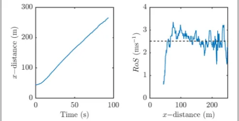
To check that the simulation is reasonable we examine the frontal position as a function of time and theRoS(ie the time derivative
FIGURE 2 |The simulation domain showing the line ignition source (red strip), and the house structure (blue object).
of the position) of the fire. The frontal location and RoS are shown inFigure 3. Because of the noise in the RoSresults, a five-point moving average smoothing was applied to the data to reveal informative trends. The frontal location in time shows a brief ignition phase over the first 5 s of the simulation before becoming approximately linear, indicative of a quasi-steady fire. TheRoSshows a slight decreasing trend after the ignition phase. The average rate of spread (∼2.2 ms−1) is commiserate with
the observations of Cheney et al. (1998), simulations of Linn et al. (2012)andMoinuddin et al. (2018), and empirical model predictions (Moinuddin et al., 2018) for similar wind speeds and fuel conditions.
The simulated heat load of the basecase, following AS 3959 as closely as possible, is compared to the AS 3959 BAL predictions. The radiative and convective heat fluxes received on all surfaces of the structure as a function of fire front distance from the structure are shown inFigure 4. Because the fire location moves over time the distances between the fire and the structure changes in time. Because AS 3959 quantifies BAL in terms of distance and because different fire parameters lead to differentRoS, these plots are made with respect to fire distance, rather than time. The
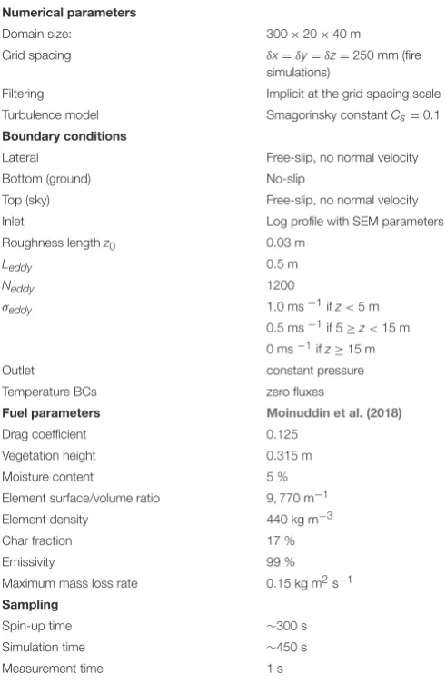
TABLE 1 |Simulation parameter values and characteristics.
Numerical parameters
Domain size: 300×20×40 m
Grid spacing δx=δy=δz=250 mm (fire
simulations)
Filtering Implicit at the grid spacing scale
Turbulence model Smagorinsky constantCs=0.1
Boundary conditions
Lateral Free-slip, no normal velocity
Bottom (ground) No-slip
Top (sky) Free-slip, no normal velocity
Inlet Log profile with SEM parameters
Roughness lengthz0 0.03 m
Leddy 0.5 m
Neddy 1200
σeddy 1.0 ms−1ifz<5 m
0.5 ms−1if 5≥z<15 m
0 ms−1ifz≥15 m
Outlet constant pressure
Temperature BCs zero fluxes
Fuel parameters Moinuddin et al. (2018)
Drag coefficient 0.125
Vegetation height 0.315 m
Moisture content 5 %
Element surface/volume ratio 9, 770 m−1
Element density 440 kg m−3
Char fraction 17 %
Emissivity 99 %
Maximum mass loss rate 0.15 kg m2s−1
Sampling
Spin-up time ∼300 s
Simulation time ∼450 s
TABLE 2 |Parameters for base case and parametric study.
Base case parameters
Driving velocity u10=12.5 ms−1
Vegetation load 0.375 kgm−2
Relative humidity 25%
Bryam Number Nc=0.6,RoS=2.3 ms−1
Driving velocity Vegetation load: 0.75 kgm−2, Relative
humidity :25 %
Vel. case 1driving velocity u10=12.5 ms−1,Nc=1.1,RoS=2.0 ms−1
Vel. case 2driving velocity u10=8.33 ms−1,N
c=3.6,RoS=1.8 ms−1
Vel. case 3driving velocity u10=5.55 ms−1,N
c=49.5,RoS=1.9ms−1
Vegetation load Driving velocity: 12.5 ms−1, Relative humidity :25 %
Veg. case 1Vegetation load 1.5 kg m−2,N
c=1.1,RoS=2.3 ms−1
Veg. case 2Vegetation load 0.75 kg m−2,N
c=1.1,RoS=2.0 ms−1
Veg. case 3Vegetation load 0.375 kg m−2,Nc=0.6,RoS=2.3 ms−1
Relative humidity Vegetation load: 0.375 kgm−2, Driving velocity: 12.5 ms−1
RH case 1Relative humidity 25%,Nc=0.6,RoS=2.3 ms−1
RH case 2Relative humidity 12.5%,Nc=1.1,RoS=2.2 ms−1
RH case 3Relative humidity 6.25%,Nc=1.1,RoS=2.2 ms−1
FIGURE 3 |The frontal location(left)andRoS(right)as a function of time. TheRoShas been smoothed using a five-point moving average. The dashed line shows the meanRoSover the simulation.
radiative heat flux on the structure is irregular, although some trends are observable. The heat flux on the front surface increases most quickly as the flame makes contact with the structure. The heat flux on the rear surface increases after the fire has passed the structure. The heat fluxes on the left and right sides both increase at the same distance (∼–10 m) but the peak radiative heat load on the left hand side is much greater than on the right hand side and on the front of the structure. The asymmetry is likely due to a complicated wake behind the structure which leads to intensification of the fire on one side of the structure. While this phenomenon is interesting, a full investigation is beyond the scope of the present study. Furthermore, the peak of radiant heat flux, when the fire is in direct contact with the structure is not important because the structure will likely ignite. The radiant heat flux on the top of the structure is minimal because the top surface is flat and not exposed to the flame. The radiation heat load can be used to estimate the duration of the heat load on the
structure. The heat load on all faces is summed and the peak total heat load is measured. The duration of heat exposure is taken as the time period where the heat load exceeds 1% of the peak total heat load. For the basecase the exposure duration is 22 s. Note that all other cases give similarly short exposure periods. The duration of exposure is important when considering ignition by radiation alone, however, in reality most house losses ignitions are piloted by embers (Blanchi and Leonard, 2005).
The convective heat flux on the structure is approximately an order of magnitude less than the corresponding radiative heat flux on the structure and therefore negligible in terms of BAL in this case. However, this does not imply that the convective heat load on the structure is always negligible nor does this imply that the increased windload due to the convective plume can be neglected.
The Byram number is computed from Equation (9) using the quasi-steady rate of spread before the fire impacts on the structure and the mean total heat release rate over the time before the fire impacts on the structure. The Bryam numbers and theRoSfrom the simulations are also listed inTable 2. The simulatedRoSare realistic compared to the grassfire experiments of Cheney et al. (1998). The simulated RoS exceeds that of previous simulations byMoinuddin et al. (2018)although we use a straight line fire as opposed to a naturally curved fire which makes significant differences to theRoS(Linn et al., 2012). The values of, and the variation in,RoScomputed here are of similar magnitude to the observations ofLinn et al. (2012). The Byram numbers indicate that most of the cases are wind dominated, except the vel. case 2, which is ambiguous and vel. case 3 which is buoyancy dominated. The Bryram numbers are unsurprising; high fuel load and low wind speed should give a buoyancy dominated fire.
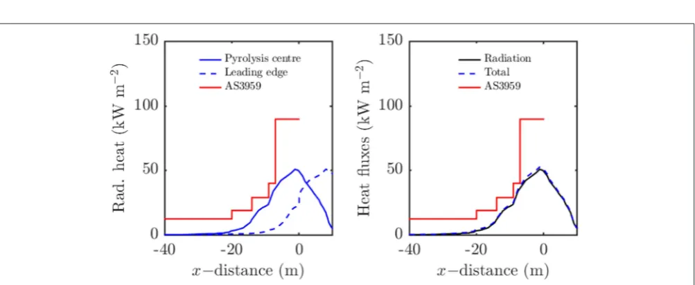
The total heat flux, that is the sum of radiant and convective heat flux, and radiation heat flux are also shown in Figure 5
FIGURE 4 |Radiation(left)and convective heat load(right)on the structure for the base case. The distance is measured to the center of the pyrolysis region.
FIGURE 5 |Comparison of heat load with AS 3959 data; the origin is the position of structure.(Left)Radiation heat load,(right)radiation and total heat load. For
(left)the fire location is estimated from the center of the pyrolysis region (fire front) and from the leading edge of the fire. For(right), only the center of the pyrolysis region is used.
flux are also shown inFigure 5to see the relative contribution of convective heat load and, as expected, the contribution of convection to total heat load is negligible in this case.
3.2. Variation of Driving Velocity
The driving wind velocity is varied with fixed vegetation load (0.75 kgm−2 and fixed relative humidity (25%). The wind
velocities are decreased from the value of 12.5 to 5.55 ms−1, or
45 to 20 kmh−1.
In this set of simulations the fuel load is high and as such a buoyancy dominated fire may be expected at low wind speeds, whereas the fire will tend to be more wind dominated at high wind speeds. Buoyancy dominated fires tend to have taller and more vertical flames than wind dominated fires, so more radiative heat load on the structure may occur at low wind speeds due to the size of the flame. Increased wind speed wind provides
increased fresh oxygen to the fire, this enhances the fuel burning rate, in turn creating a larger fire. If the shear force from the wind is significant relative to the buoyant force from the fire plume, the increased wind speed also inclines the fire plume at a more acute angle, increasing heat transfer to the virgin fuel, subsequently increasing the pyrolysis region and fire intensity. Because the fire intensity increases the flame height and flame temperature both increase leading to greater radiative heat load on the structure. However, if the fire becomes wind dominated (i.e., wind shear dominates buoyancy forces) the flame will effectively attach to the ground (Sharples et al., 2010) leading to a very small flame height and a decrease in radiative heat load on the structure.
Figure 6 shows the heat load with varying wind velocities; 5.55, 8.33, and 12.5 ms−1, respectively. The figure supports the
FIGURE 6 |Radiation heat load on the front of the structure as the wind velocity varies. Distance is measured to the pyrolysis center.
load for the 12.5 ms−1case is systematically lower than the other
two cases. The radiative heat load at distance 0 m (i.e., where the flame makes contact with the structure) for the 5.55 and the 8.33 ms−1 case wind speed case is∼90 kWm−2. However,
for the 12.5 ms−1 wind speed case the radiative heat load at
distance zero is much lower than the other two cases: ∼45 kWm−2. Unexpectedly, the intermediate wind speed 8.33 ms−1
case yields the highest heat load, suggesting that the radiative heat load dependence on the fire dynamics is complicated. For example buoyancy dominated fires with very upright flames may not burn as intensely as a buoyancy dominated fire with a slightly inclined flame. The inclination of the flame will lead to increased preheating and pyrolysis of unburnt fuel and a more intense fire overall, while still yielding a large flame area that enhances radiative heat fluxes on the structure. A more comprehensive investigation of the flame dynamics is required to fully understand this behavior.
The maximum convective heat flux on the structure was measured to be∼7% of the maximum radiative heat flux on the structure, consistent with the findings inFigure 4.
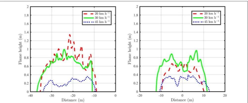
The flame profiles are examined when the fire is located atx≈ −20 m andx≈0 m. Here we use the term flame profile to refer to a cross section of the flame determined from the stoichometric mixture fraction contour and are shown in Figure 7. Because FDS uses a mixed-is-burnt combustion model these contours in thexz−plane represent the simulated flame boundary, with
combustion occurring in the region enclosed by the contours. The three fires atx= −20 m have different characteristics. For theu10 = 5.55 andu10 = 8.33 ms−1 cases the average flame
height is∼0.75 m, whereas for theu10 = 12.5 ms−1 case the
flame height is less than 0.5 m. This is consistent with the notion that theu10 =12.5 ms−1case is wind dominated and the other
two cases are buoyancy dominated. When the fire is atx=0, the flame height behavior is no longer systematic, which is likely due to the complexities of the fire engulfing the structure.
The AS 3959 model predicts that the flame height increases monotonically with wind speed. In these cases the GFDI =
34, 50, and 92 foru10 = 5.55, 8.33, and 12. ms−1respectively.
AS 3959 considers tussock moorland fires atGFDI=50 and the computedGFDIvalues are in the very high to severe fire danger rating categories. Basic manipulation of Equations (1)–(5), i.e., substituting all quantities into Equation (5) and assuming onlyu
varies gives the following equation forLf
Lf =0.0775Be0.0185u10, (11)
whereBis a constant:
B=
3.35w2H
36 exp(−0.097mc)) 0.46
mc≤18.8%, 0.299w2H
36 exp(−1.686mc)(30−mc) 0.46
18.8%<mc<30%. (12)
RecallLf is the flame length,His relative humidity,mcis fuel
moisture content, andu10is the driving wind speed.
Because the ground is flat the view factor will be maximized at α = π/2. Therefore, Lf is the only variable in Equation
(8). Hence the AS 3959 model predicts that the (maximum possible) radiation flux at the structure will increase with increasing wind speed; this prediction is not supported by these simulations. The predictions of the standard are also breached, for all wind speed cases, with the exception of the BAL-40 region in the 12.5 ms−1 case. The maximum heat flux (from
the 8.33 ms−1 cases) received in the BAL-19 region is ∼30
kWm−2, 100 kWm−2 in the BAL-29 region, and 150 kWm−2
in the BAL-40 region not breached in this case. Not correctly predicting the worse-case scenario is a problem for the standard. Structures may be built to withstand the predicted worse-case scenario and receive far greater heat flux from a fire with lowerGFDI.
3.3. Variation of Vegetation Load
Because the base case (wind speed 12.5 ms−1, 25% relative
humidity, and a fuel load of 0.375 kgm−2) is wind dominated,
increasing the fuel load should increase the intensity of the fire, and subsequently the radiative heat flux at the structure should increase. The results shown in Figure 8 support the aforementioned hypothesis. The general trend is that the radiative heat flux at the structure increases with increasing heat load; especially before the fire impacts upon the structure. There is a peak in radiative heat flux in the highest fuel load case, at around x = −20 m. The exact cause of the peak is not investigated, but the peak in radiation heat flux corresponds to a peak in total heat release rate suggesting that fire has instantaneously flared up around that point.
3.4. Variation of Relative Humidity
FIGURE 7 |Flame profiles showing characteristics of the flame at different velocities.(Left)Flame profiles at 20 m distance,(right)flame profiles at the structure location.
FIGURE 8 |Radiation heat load on the front of the structure with varying vegetation load. Distance is measured to the pyrolysis center.
parameters, we modify the relative humidity without changing the fuel moisture content. Three relative humidities are selected: 6.25, 12, and 25% (basecase) with wind speed and fuel load held constant at 12.5 ms−1and 0.375 kgm−2, respectively. The
results in these cases are complicated: the relative humidity (with constant fuel moisture content) does modify the radiative heat flux at the structure however the results are not completely systematic. The general trend is that lower relative humidity yields the peak higher radiative heat load as shown inFigure 9. However, the 25% relative humidity case yields the highest radiative heat flux when −20 < x < −10 m. At x = −15 m the 25% case gives radiative heat flux of∼30 kWm−2,
the 12% case gives radiative heat flux of ∼22 kWm−2, and
FIGURE 9 |Radiation heat load on the front face of the structure as a function of distance to the flame center with varying relative humidity. Distance is measured to the pyrolysis center.
the 6.25% case gives radiative heat flux of ∼18 kWm−2.
3.5. The Case to Improve Building
Standards With Physics-Based Modeling
Designing building standards is arguably a very difficult task. In the case of building in bushfire prone areas, the basic requirements of the standard are to ensure that a building is resilient to a realistic fire event and the standard is simple and straightforward to apply. Idealized simulations, such as those conducted here, can be considered as a first attempt at providing a framework that can be used to revise existing standards. Controlled physical experiments can also serve as a validation for proposed structural integrity discussed in AS 3959 in a bushfire attack. The controlled experiments have significant cost, risk, and safety, which limits it utilization. Numerical modeling reduces the cost, risk, and safety in exploring the bushfire attack on structure. Previously, numerical simulations have been successfully applied to simulate experimental grassfires (Mell et al., 2007; Moinuddin et al., 2018). Here, we have demonstrated that the same physics-based models can simulate the radiant heat load upon a structure. The computational effort required to simulate fire impact on a structure is currently too great to allow the possibility of simulating a general proposed structure in a given location in detail. However in the future, simulation of fire impact on a proposed design may become part of the design and approval process.For the data presented here, the idealized models included in AS 3959 were found to under predict the simulations results near the structure. Furthermore, the models in AS 3959 do not account for the differences between buoyancy dominated and wind dominated fires. Given these limitations and the omission of any kind of ember attack model, in the AS 3959 the standard should be re-examined.
Because computational technology and physics-based simulation have advanced considerably since the standard was originally implemented, physics-based simulations of bushfire attack on a structure could be used to strengthen the standard. It is important to examine the limitations of the approach presented here. Firstly, it is unlikely that a house structure would be built in unmaintained grasslands; most houses have a garden with watered or mowed grass forming a buffer region from the fire. Nonetheless the simulations conducted here reflect the situations outlined in AS 3959. The present research only considers surface fuels whereas the standard is mostly concerned with elevated forest or shrub like fuels. In planning this study, it was thought that surface fuels were likely to be better predicted by the idealized model used by the standard. The geometry of the vegetation, the possibility of crown fuel involvement, and wind reduction due to the vegetation are expected to complicate the fire impact upon a structure. Similarly this study did not address the effect of sloping terrain on the fire spread and radiative heat load. Therefore, a further study should be conducted in future to address these limitations.
4. CONCLUSIONS
Physics based simulations are performed following the model outlined in the building standard AS 3959. The basecase simulation was designed to replicate the AS 3959 grassland
(tussock moorland) fire as close as computationally feasible. That is, a straight line fire approaching a small cubiod structure was simulated and the radiative heat flux at the front face of the structure was analyzed as a function of the distance from fire front to the structure. The AS 3959 standard is based upon the radiative heat flux received at the structure. The standard sets several BAL levels; the BAL level is the radiative heat flux permitted if the fire is a particular difference away from the structure. Due to computational constraints, the width of the simulated fire is 20 m instead of the 100 m outlined in the standard. As the fire width increases, the radiative heat flux on the structure should also increase. The simulated radiative heat flux was similar in magnitude to the modeled radiative heat flux. However, the simulation was conducted at a much smaller width than the standard considers. Because radiative heat flux will increase with increasing fire width, therefore, the standard is likely insufficient for these fires. A parametric study shows that the relative humidity alone does vary the radiative heat flux on a structure, but not entirely in a systematic manner. Relative humidity will also vary the fuel moisture content, held constant in these simulations, and effect of varying the fuel moisture content needs to be investigated. The fuel load increases the radiative heat flux on a structure. As wind speed increases the fire changes from a buoyancy dominated fire leading to high radiative heat flux upon a structure, to a wind dominated fire with lower heat flux on the structure and this occurs despite theGFDI
monotonically increasing.
Overall, building standards based on radiative heat flux alone will require revision to account for other forms of bushfire impact such as ember attack. Physics based modeling has the potential to simulate realistic fires and physics based simulations could be used to revise the radiative heat flux levels used in AS 3959. As computational capacity increases, physics based simulations may be used in performance based design of structures in bushfire prone areas.
AUTHOR CONTRIBUTIONS
NK conducted and analyzed the bulk of the simulations presented in this work and contributed to writing the manuscript. DS conducted preliminary simulations, proposed the study presented, and contributed writing the manuscript. RW conducted a literature review, performed an assessment of AS 3959, and contributed to writing the manuscript. KM contributed to writing the manuscript and provided guidance and expertise throughout the project.
FUNDING
This project was funded by the Commonwealth of Australia through the Bushfire and Natural Hazards Cooperative Research Centre. Project: Fire spread prediction across fuel types, 2014–2020.
ACKNOWLEDGMENTS
REFERENCES
Apte, V., Bilger, R., Green, A., and Quintiere, J. (1991). Wind-aided turbulent flame spread and burning over large-scale horizontal pmma surfaces.Combust. Flame
85, 169–184. doi: 10.1016/0010-2180(91)90185-E
AS 3959 (2009).Construction of Buildings in Bush Fire Prone Areas (as 3959). Technical report, Standards Australia, Sydney, NSW.
Blanchi, R., and Leonard, J. (2005).Investigation of Bushfire Attack Mechanisms Resulting in House Loss in the Act Bushfire 2003. Technical report, Bushfire Cooperative Research Centre (CRC) Report.
Bou-Zeid, E., Overney, J., Rogers, B. D., and Parlange, M. B. (2009). The effects of building representation and clustering in large-eddy simulations of flows in urban canopies. Bound. Layer Meteorol. 132, 415–436. doi: 10.1007/s10546-009-9410-6
Cheney, N., Gould, J., and Catchpole, W. R. (1998). Prediction of fire spread in grasslands.Int. J. Wildland Fire8, 1–13. doi: 10.1071/WF9980001
Cruz, M. G., and Alexander, M. E. (2013). Uncertainty associated with model predictions of surface and crown fire rates of spread.Environ. Model. Softw.
47, 16–28. doi: 10.1016/j.envsoft.2013.04.004
Dold, J., and Zinoviev, A. (2009). Fire eruption through intensity and spread rate interaction mediated by flow attachment.Combust. Theor. Model.13, 763–793. doi: 10.1080/13647830902977570
Jarrin, N., Benhamadouche, S., Laurence, D., and Prosser, R. (2006). A synthetic-eddy-method for generating inflow conditions for large-eddy simulations.
Int. J. Heat Fluid Flow 27, 585–593. doi: 10.1016/j.ijheatfluidflow.200 6.02.006
Jolly, W. M., Cochrane, M. A., Freeborn, P. H., Holden, Z. A., Brown, T. J., Williamson, G. J., et al. (2015). Climate-induced variations in global wildfire danger from 1979 to 2013.Nat. Commun.6:7537. doi: 10.1038/ncom ms8537
Linn, R., Canfield, J., Cunningham, P., Edminster, C., Dupuy, J.-L., and Pimont, F. (2012). Using periodic line fires to gain a new perspective on multi-dimensional aspects of forward fire spread.Agric. For. Meteorol.157, 60–76. doi: 10.1016/j.agrformet.2012.01.014
McArthur, A. G. (1967).Fire Behaviour in Eucalypt Forests. Leaflet number 107. McGrattan, K., Hostikka, S., and Floyd, J. (2013a).Fire Dynamics Simulator, User’s
Guide. Gaithersburg, MD: NIST special publication, 1019.
McGrattan, K., Hostikka, S., Floyd, J., Baum, H. R., Rehm, R. G., Mell, W., et al. (2013b).Fire Dynamics Simulator (Version 6), Technical Reference Guide. Gaithersburg, MD: NIST special publication, 1018.
McLeod, R. N., Pascoe, S. M., and Teaguea, B. G. (2010).Final Report, Royal Commission into Victoria’s Bushfires. Technical report, State of Victoria. Mell, W., Jenkins, M. A., Gould, J., and Cheney, P. (2007). A physics-based
approach to modelling grassland fires. Int. J. Wildland Fire 16, 1–22. doi: 10.1071/WF06002
Mell, W., Maranghides, A., McDermott, R., and Manzello, S. L. (2009). Numerical simulation and experiments of burning douglas fir trees.Combust. Flame156, 2023–2041. doi: 10.1016/j.combustflame.2009.06.015
Mell, W. E., McDermott, R. J., and Forney, G. P. (2010). “Wildland fire behavior modeling: perspectives, new approaches and applications,” inProceedings of 3rd Fire Behavior and Fuels Conference(Birmingham, AL), 25–29.
Moinuddin, K., Sutherland, D., and Mell, W. (2018). Simulation study of grass fire using a physics-based model: striving towards numerical rigour and the effect of grass height on the rate of spread.Int. J. Wildland Fire27, 800–814. doi: 10.1071/WF17126
Morvan, D., and Dupuy, J. (2004). Modeling the propagation of a wildfire through a mediterranean shrub using a multiphase formulation.Combust. Flame138, 199–210. doi: 10.1016/j.combustflame.2004.05.001
Morvan, D., and Frangieh, N. (2018). Wildland fires behaviour: wind effect versus byram’s convective number and consequences upon the regime of propagation.
Int. J. Wildland Fire27, 636–641. doi: 10.1071/WF18014
Morvan, D., Meradji, S., and Mell, W. (2013). Interaction between head fire and backfire in grasslands.Fire Saf. J.58, 195–203. doi: 10.1016/j.firesaf.2013.01.027 NFPA 1144 (2013).Nfpa 1144 Standard for Reducing Structure Ignition Hazards from Wildland Fire. Technical report, National Fire Protection Association and others.
Radeloff, V. C., Hammer, R. B., Stewart, S. I., Fried, J. S., Holcomb, S. S., and McKeefry, J. F. (2005). The wildland–urban interface in the united states.Ecol. Appl.15, 799–805. doi: 10.1890/04-1413
Radeloff, V. C., Helmers, D. P., Kramer, H. A., Mockrin, M. H., Alexandre, P. M., Bar-Massada, A., et al. (2018). Rapid growth of the us wildland-urban interface raises wildfire risk.Proc. Natl. Acad. Sci. U.S.A.115, 3314–3319. doi: 10.1073/pnas.1718850115
Roberts, M., Sharples, J., and Rawlinson, A. (2017). “Incorporating ember attack in bushfire risk assessment: a case study of the Ginninderry region,” in
MODSIM2017 Proceedings - MSSANZ, Modelling and Simulation Society of Australia and New Zealand, The 22nd International Congress on Modelling and Simulation(Hobart, TAS), 1152–1158.
Ronchi, E., Gwynne, S. M., Rein, G., Wadhwani, R., Intini, P., and Bergstedt, A. (2017).e-Sanctuary: Open Multi-Physics Framework for Modelling Wildfire Urban Evacuation. Technical report, National Fire Protection Association. Rüedi, I. (2006).WMO Guide to Meteorological Instruments and Methods of
Observation: WMO-8 Part i: Measurement of Meteorological Variables. Geneva: World Meteorological Organization.
Sharples, J. J. (2017).Risk Implications of Dynamic Fire Propagation. Report for Ginninderra Falls Association (Non-peer reviewed report).
Sharples, J. J., Gill, A. M., and Dold, J. W. (2010). “The trench effect and eruptive wildfires: lessons from the kings cross underground disaster,” inProceedings of Australian Fire and Emergency Service Authorities Council 2010 Conference
(Darwin, NT), 8–10.
Tollhurst, K. (2009).Report on the Physical Nature of the Victorian Fires Occurring on the 7th of February 2009. Technical report, University of Melbourne. Viegas, D. X. (2017).O Complexo de Incéndios de Pedr og ao Grande e Concelhos
limtrofes, Iniciado a 17 de Junho de 2017. Technical report, Universidade de Coimbra.
Weise, D., and Biging, G. (1996). Effects of wind velocity and slope on flame properties.Can. J. For. Res.26, 1849–1858. doi: 10.1139/x26-210
Whittaker, J., Haynes, K., Handmer, J., and McLennan, J. (2013). Community safety during the 2009 Australian ‘Black Saturday’ bushfires: an analysis of household preparedness and response.Int. J. Wildland Fire 22, 841–849. doi: 10.1071/WF12010
Worden, H., Beer, R., and Rinsland, C. P. (1997). Airborne infrared spectroscopy of 1994 western wildfires. J. Geophys. Res. Atmos. 102, 1287–1299. doi: 10.1029/96JD02982
Conflict of Interest Statement: The authors declare that the research was conducted in the absence of any commercial or financial relationships that could be construed as a potential conflict of interest.
NOMENCLATURE
Symbols
w fuel weight (T/Ha)
mc fuel moisture content (percentage)
u driving wind speed (ms−1)
RH relative humidity (percentage)
C the curing index (percentage)
Nc Byram number
Lf flame length (m)
Fh flame height (m)
Fw flame width (m)
α flame angle
Tf flame temperature (K)
Ta is the ambient temperature (K)
ǫ emissivity (unitless 0 to 1)
q heat flux (kW/m2)
z0 roughness length (m)
A Imposed velocity magnitude (inlet condition) (ms−1)
Leddy eddy length scale (inlet condition)
Neddy number of eddies (inlet condition)
σeddy velocity scale of eddies (inlet condition)
δx,δy,δz grid sizes inx,y, andz
Standard constants
σ=5.67×10⁻⁸W/m2K4 Stefan-Boltzmann constant
g=9.8 ms−2 gravitation acceleration constant
ρ=1.2 kg/m3 density of air
Cp=1.0 kJ/kg K specific heat of air
H=18.6 MJ kg−1 heat of combustion
Subscripts
inlet atx=0
eddy pertaining to the synthetic inlet turbulence
10 measured ten meters from the ground
r radiant
emitted emitted from the flame