Optimized optical setup for DIC in rock mechanics

Optimized optical setup for DIC in rock mechanics

D.S. Yang1, M. Bornert2,a, H. Gharbi1, P. Valli1,and L.L. Wang1

1 _{Laboratoire de Mécanique des Solides, École Polytechnique ParisTech, 91128 Palaiseau, France}

2 _{Unité de Recherche Navier, École des Ponts ParisTech, 77544 Marne-la-Vallée, France}

Abstract. In order to investigate the micromechanical mechanisms of argillaceous rocks under combined mechanical load and varying moisture, and observe very low strain rates of about 10-10 _s-1_{, i.e. about 10}-4 _{per week, a specific optical setup for Digital}

Image Correlation (DIC) has been developed at the Solids Mechanics Laboratory, Ecole Polytechnique. This paper mainly presents two procedures to optimize the experimental setup and enhance the full-field strain measurement accuracy. The first one allows us to minimize the systematic DIC errors by choosing an optimal optical setup, including appropriate lens aperture and light source with small wavelength, in combination with a specific grey level interpolation method (bilinear, bicubic, biquintic) in DIC algorithms. The second procedure aims at reducing the errors induced by overall out-of-plane motions of the sample. This procedure makes use of a specifically designed optical microscope, which tracks the few tens of micrometers out-of-plane motions of the sample all along the several months lasting test, to compensate the magnification fluctuations which disturb the macroscopic measurements. The current optimized optical setup gives a better than 10-5 accuracy at macro scale (3 mm gage length) and 10-4 accuracy at microscale (about 100 µm gage length).

1 Introduction

While Digital Image Correlation (DIC) techniques are widely used to investigate the mechanical properties of structural materials such as metals, polymers and composites [1], much fewer applications in rock mechanics are reported. The main reason is probably the very low strain levels such materials sustain before failure or macroscopic localization, typically below 10-3 or even less. For instance, the creep behaviour of argillaceous rock, which is considered as a potential host rock for nuclear waste repository and is under investigation in the present study, is typically characterised by strain rates of about 10-10 s-1, i.e. about 10-4 per week. In order to identify and characterise the micro-mechanisms of creep, accuracies in terms of strain measurements of the order of 10-5 are required over long periods of time, not only at the macroscopic scale of the centimetric sample but also at the local scales at which such mechanisms are suspected to act.

The developed experimental setup combines a controlled hydro-mechanical loading device with real time continuous optical observations at both the scale of the sample and the scale of the microstructure. It extends an earlier simpler setup in which only mechanical load was controlled on

a

Email : [email protected]

© Owned by the authors, published by EDP Sciences, 2010 DOI:10.1051/epjconf/20100622019

samples preliminarily subjected to and in equilibrium with an atmosphere at a fixed relative humidity prescribed by a saturated saline solution [2].

This paper starts with a short presentation of the experimental setup, which will be described in detail elsewhere [3], and then focuses on two specific procedures which have been developed to improve the accuracy of optical measurements. The first procedure aims at precisely quantifying actual systematic DIC errors obtained with the images in use and then reducing the amplitude of these errors by an appropriate choice of the lens aperture, which controls the size of diffraction patterns, so as to adapt it to the available natural contrast of the rock used as DIC patterns and the specific DIC algorithm. The second one consists in correcting the errors induced by the overall micrometric out-of-plane motion of the sample on the macroscopic DIC measurements. Indeed, because of geometric constraints, stereo-correlation techniques can hardly be applied in the present context. The alternative solution consists in tracking the motion of the sample with the optical microscope specifically designed to investigate deformations at microscale. A contrast detection algorithm automatically keeps the microscope in focus and centres the area of interest; it records in addition the distance between the sample and the macroscopic camera with micrometric accuracy.

2 Experimental setup

The experimental setup mainly consists of three parts: macroscopic and microscopic optical setups; mechanical loading device; suction control equipment.

The macroscopic DIC setup (MacroDIC) employs a 16 Megapixels ImperX progressive scan CCD camera, which is equipped with a Schneider 5.6/120 APO Componon macrolens. This camera records images of the whole surface of the sample (24x36 mm) with 4872x3248 pixels in 12 bits (1 pixel = 7.4 µm). The lens exhibits very low geometric distortion at the optical magnification equal to one in use (CCD-sample distance = 480 mm). Two groups of four blue (wavelength λ = 440-490 nm) Light Emitting Diodes (LED) symmetrically and uniformly illuminate the flat surface of the sample with an incident angle of about 45 degrees. The blue LEDs with shorter wavelength have been preferred to red, green or even white LEDs because they provide a larger depth of field (about 1 mm) for a given diffraction pattern size, the latter playing an important role in the optimization of the setup as shown later. In addition, blue light is close to the peak quantum efficiency of the sensor. The camera is mounted on a manual X-Y-Z translation stage with about 10 µm positioning accuracy. This macroscopic optical setup is fixed during the hydromechanical loading.

The microscopic optical setup (MicroDIC) consists of a 4 Megapixels Diagnostic Instruments Spot Insight IN1400 digital camera, an infinity-corrected Mitutoyo apochromatic 10 objective lens and a 200mm MT1 optical tube lens. With this optical combination, the observed object area is 1.5x1.5 mm and the pixel size 0.74 µm, to be compared with the 1 µm optical resolution of the lens (numerical aperture α = 0.28). The working distance is 34 mm. In consideration of the small depth of field of optical microscopy, about 3.5 µm, the camera has been mounted on a servo-controlled micrometric X-Y-Z translation stage. With this servo-control, Z position (normal to sample) is automatically adjusted for sharp focus, by means of a contrast maximization algorithm, and the camera can be moved automatically along X and Y directions to observe several juxtaposed zones and centre them on positions of interest by means of standard DIC algorithms. Because of mechanical limitations of the translation stages, the accuracy of this positioning is currently limited to 3 µm but will be reduced to 0.1 µm for the Z translation in a near future. The normal and lateral white illuminations described in [2] are used. An additional manual rotation stage is used to align the X-Y translation stage with the surface of the sample so that focus is kept when the microscope is moved all over the whole flat surface.

normal to these flats is 26.8 mm. Teflon sheets are used to reduce fretting effects at the sample/machine interface and moments are reduced by means of a spherical bearing.

Relative humidity is prescribed by means of supersaturated saline solutions which are placed near the sample inside an airtight PMMA container, about 25x25x40 cm in size, in which holes have been machined for the optics and the loading line. The whole system is illustrated in Fig.1

Fig.1. Macroscopic and microscopic optical setup for the coupled hydro-mechanical tests of rocks

3 Minimizing the systematic DIC errors

3.1 Systematic errors

direct determination of the S-shaped curve by means of a simple and single out-of plane motion. It is used to determine an optimal aperture of the lens which leads to a reduction of this error.

3.2 Determining the systematic errors and the dependence with aperture

With standard (non-telecentric) lenses a relative motion dZ of the camera with respect to the sample along the optical axis, without refocusing, generates a relative magnification variation of the image equal to -dZ/OC where OC is the object-to-optical center distance, equal to 240 mm on our MacroDIC setup. If dZ is sufficiently small, so that both images, recorded before and after translation, are in focus, their image characteristics are identical. The 2D apparent motion generated by such a 3D motion is a radial displacement with respect to some motionless pixel close to the optical center. The relative translation of one side of a W pixels wide ROI with respect to the other is Du = W.dZ/OC, while within a correlation window of width w pixels, maximal relative motion is du = w.dZ/OC. As W>>w (typically 4000 pixels with respect to 30 in our setup), one can chose dZ such that du is sufficiently small within a correlation window and the displacement associated with a constant systematic error, i.e. a single point on the S-shaped curve, and such that, at the same time, Du is equal to a few unities, such that all positions of the S-shaped curve are explored several times in one image, both in X and Y directions. In practice, for our setup, dZ can vary from 100 to 500 µm, generating 2 to 10 fringes in X and 1 to 7 fringes in Y in the apparent deformation maps. It is rather easy to determine the parameters of the radial motion from the measured displacement of points at the boundary of the ROI. Care can in addition be taken to select the ROI such that points at its boundary suffer from the same systematic error, so that the evaluations of the apparent isotropic strain in not affected by this error. The comparison between the homogeneous radial motion and the DIC-measured motion at any position inside the ROI, analysed as a function of the fractional part of the X and Y components of the theoretical displacement, gives then a direct access to the systematic errors. Random errors are also available, but not discussed here. It is checked that the obtained curve does not depend on dZ, as soon as images are in focus, demonstrating the intrinsic nature of the results. Dependence of these actual experimental errors on various parameters such as window size, correlation algorithms, but also image characteristics can then be investigated. In the following, we focus on the importance of lens aperture, with respect to actual sample contrast and DIC grey-level interpolation algorithms.

Indeed the contrast on the digital images can be strongly changed when lens aperture is changed, all other parameters being unchanged except the exposure time modified so as to keep a constant illumination of the sensor (and thus same shot noise levels). A smaller aperture increases the depth of field, but enlarges diffraction patterns, characterized by the Airy disc radius equal to 0.61 λ /α. Fig.2. and Fig.3. present the typical evolution with aperture of the contrast of digital images. The natural contrast of the argillaceous rock, essentially made of a clay matrix and quartz or calcite grains 10 to 50µm in diameter [2], is shown in Fig. 2 while the artificial contrast of an aluminium sample marked with a speckle painting, is presented in Fig. 3. Aperture A1 corresponds to full open (f-number equal to 5.6 when the lens is focused at infinity) and an increase of one unity corresponds to a division by two of the light flux. The smaller aperture clearly leads to smoother images.

A1 A2 A3

A4 A5 A6

Fig.2. Natural contrast of argillaceous rocks (60 x 90 pixels) observed with various apertures

A1 A2 A3

A4 A5 A6

Fig.3. Artificial contrast by sprayed paint of an aluminium sample (80 x 90 pixels) at various apertures

-0.10 -0.08 -0.06 -0.04 -0.02 0.00 0.02 0.04 0.06 0.08 0.10

0 0.2 0.4 0.6 0.8 1

Interpolation - bilinear

Aperture -2 Aperture -3 Aperture -4 Aperture -5 Aperture -6

Subpixel position (pixel)

E

rr

o

r

(p

ix

e

l)

(a)

-0.04 -0.03 -0.02 -0.01 0.00 0.01 0.02 0.03 0.04

0 0.2 0.4 0.6 0.8 1

Interpolation - biquintic

Aperture -2

Aperture -3

Aperture -4

Aperture -5

Aperture -6

E

rr

o

r

(p

ix

e

l)

Subpixel position (pixel) _(b)

Fig.4. Systematic errors as a function of lens aperture, DIC with bilinear interpolation (a) and biquintic interpolation (b), Schneider 5.6/120 APO Componon lens, natural contrast of an argillaceous rock

3.3 Effect of the interpolation method on the systematic errors

associated with a given interpolation, there is indeed little difference of the errors for these three interpolations. The choice of interpolation scheme can then be governed by other considerations, such as depth of field (i.e. small aperture and small order interpolation) or spatial resolution (large aperture and higher order interpolation).

-0.08 -0.06 -0.04 -0.02 0.00 0.02 0.04 0.06

0 0.2 0.4 0.6 0.8 1

Aperture -3

Bilinear Bicubic Biquintic

Subpixel position (pixel)

E rr o r (p ix e l) (a) -0.06 -0.04 -0.02 0.00 0.02 0.04 0.06

0 0.2 0.4 0.6 0.8 1

Aperture -6

Bilinear

Bicubic

Biquintic

Subpixel position (pixel)

E rr o r (p ix e l) (b)

2 (a) and a lens aperture 6 (b), natural contrast of an argillaceous rock

-0.03 -0.02 -0.01 0.00 0.01 0.02 0.03

0 0.2 0.4 0.6 0.8 1

Interpolation - bilinear

Aperture -2 Aperture -3 Aperture -4 Aperture -5 Aperture -6

Subpixel position (pixel)

E rr o r (p ix e l) (a) -0.04 -0.03 -0.02 -0.01 0.00 0.01 0.02 0.03 0.04

0 0.2 0.4 0.6 0.8 1

Aperture -6

Bilinear Bicubic Biquintic

Subpixel position (pixel)

E rr o r (p ix e l) (b)

Fig.6. Systematic errors as a function of lens aperture (a) and their variations under three different interpolations

for lens aperture 6 (b); artificial speckle pattern on the surface of an aluminium sample

The same phenomena have been found on the aluminium sample with the artificial speckel pattern. The results however show that the systematic errors depend on the actual “physical” contrast of sample. Optimal aperture for bilinear interpolation now turns out to be between 3 and 4, with amplitude of systematic error below 0.01 pixels, lower than that obtained with the natural contrast of the rock sample (Fig. 6.a). The little or even bad influence of high order interpolation on the systematic errors is observed again in some circumstances (Fig.6b).

With these procedures, it is possible to optimize the amplitude of systematic error so as to keep them lower than random errors, which are essentially linked to image noise and correlation window sizes, and are of the order of 0.01 pixels (with 30 pixels wide correlation windows). Under such conditions, the MacroDIC setup provides an accuracy better than 10-5, over a gage length of 3 mm (~400 pixels, i.e. 8x12 independent strain measurements on the sample). This is a 10-fold accuracy improvement with respect to the earlier setup [2] which is required to investigate very low creep strain rates.

4 Reducing the effect of out-of-plane motions on DIC measurements

the sample. This is in particular the case on our setup where the loading device is not very rigid transversally because of the presence of the airtight container which requires a “long” loading system. These motions will induce a magnification variation on the MacroDIC images, which depend linearly on the out-of-plane motion as already emphasized in section 2 and as predicted by a simple pinhole projection model, or basic geometric optics. Sutton et al [9] presented a more general evaluation of the effect of out-of-plane motion (including out-of-plane translation and rotation) and compared it with the experimental one.

Simple considerations will however be sufficient for our needs. The magnification variation induces a multiplicative factor on the 2D deformation gradient so that the apparent gradient is Fa = Fg. F,

where F is the real gradient (second order tensor), and Fg = (1 + ∆g/g)1 is due to the magnification

variation ∆g between the two images. In this expression g is the magnification and 1 the identity tensor. Under the small strain assumption, an additive relation on linearized strains is obtained : ε = ε

ε = ε ε = ε

ε = εa - ∆g/g1, where εεεε is the real in-plane strain and εεεεa the apparent one provided by DIC. As

already mentioned, the magnification variation linearly depends on the sample-camera distance according to ∆g/g = -dZ/OC. The object-to-optical center distance OC can be determined experimentally with high accuracy by plotting the magnification variation computed by DIC as a function of the measured motion of the camera, prescribed with the available manual Z-stage, following a procedure very similar to that described in section 3.

The difficulty is now to evaluate accurately the overall dZ displacement of the sample during the hydro-mechanical test (recall that during the test, the MacroDIC camera does not move). In this study, we make use of the available MicroDIC setup and its already-described automatic focusing system to record the motion of the flat surface of the sample opposite the MacroDIC. Focusing is based on contrast detection and makes use of the low 3.5µm depth of field of the microscope. Several tens of micrometers out of plane motion of the sample are recorded this way all along the several months lasting test on the microDIC side. Combining this measured motion dZmicro and the

transverse deformation of the sample (Fig.7.), the relative displacement of the other side of the sample with respect to the fixed macroscopic lens can be evaluated with micrometric resolution according to dZ = dZmicro

+ D

the sample. As the rock can be considered transversly isotropic about the load axis (which is normal to bedding planes) the overall transverse strain εzz can reasonably be assumed equal to the transverse in-plane strain εyy, so that dZ = dZmicro

+ D

apparent εyya and real εyy transverse in-plane strains, the dZmotion andsubsequently to all corrected

strain components.

zmicro_{_deformed}

Microscopic Lens

Macroscopic Lens Object

zmacro

zmicro

Fig.7. Scheme of the out-of-plane motions during the test

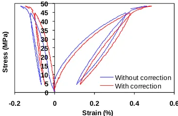
0 5 10 15 20 25 30 35 40 45 50

-0.2 0 0.2 0.4 0.6

S

tr

e

s

s

(

M

P

a

)

Strain (%)

Without correction With correction

Fig. 8. Magnification correction on overall DIC-strain/stress curve

5 Conclusions

An experimental setup, which combines a controlled hydro-mechanical loading device with a multi-scale full-field measurement setup by DIC, has been developed to investigate the deformation of argillaceous rocks under coupled hydro-mechanical conditions.

In order to observe very low creep strain rates and improve the measurement accuracy, two procedures have been developed. The first one allows to minimize the systematic DIC errors by choosing an optimal lens aperture and blue light as the illumination source. Moreover, the comparison of three interpolation methods shows that the higher order interpolations schemes are not always better than a simple bilinear interpolation but that optimal combinations can be found. The second one uses an optical microscope not only to observe several juxtaposed 1.5 x 1.5 mm fields, but also follow the out-of-plane motions with micrometric accuracy. The later characteristic of the microscope can be used to compensate magnification variations induced by the out-of-plane motions. The experimental tests confirm that these are efficient procedure to reduce the errors. These procedures are currently under daily use to determine the evolution of elastic and nonlinear properties of argillaceous rocks under combined hydro-mechanical loads.

5 Acknowledgments

This research was funded by ANDRA and the authors gratefully acknowledge this support.

References

1. M.A. Sutton, J.J. Orteu, H.Schreier. Image Correlation for Shape, Motion and Deformation Measurements (Springer, 2009)

2. M. Bornert, F. Valès, H. Gharbi, D. Nguyen Minh, Strain, 46, 33-46 (2010)

3. D.S. Yang, M. Bornert, D. Nguyen Minh, S. Chanchole, H. Gharbi, P. Valli, Clays in Natural & Engineered Barriers for Radioactive Waste Confinement, Nantes, (2010)

4. S. Choi, S. Shah, Exp. Mech., 37/3, pp. 307-313 (1997)

5. P. Doumalin, M. Bornert, D. Caldemaison, Proc. of ATEM99, pp. 81–86, (1999) 6. H. Schreier, J. Braasch, M.A. Sutton, Opt. Eng. 39/11, pp. 303–311 (2000)

7. Y. Q. Wang, M. A. Sutton, H. A. Bruck, H. W. Schreier, Strain 45, 160–178, (2009). 8. J.C. Dupré, , M. Bornert, L. Robert, B. Watrisse, this conference.