Available Online at www.ijcsmc.com
International Journal of Computer Science and Mobile Computing
A Monthly Journal of Computer Science and Information Technology
ISSN 2320–088X
IMPACT FACTOR: 5.258IJCSMC, Vol. 5, Issue. 7, July 2016, pg.509 – 514
Numerical Solution of Volterra
Integral Equations of Second Kind
Jumah Aswad Zarnan
Asst. Prof. Dr., Dept. Of Accounting by IT, Cihan University \ Campus \ Sulaimaniya, Iraq
Abstract— In the present paper, we solve numerically Volterra integral equations of second kind with regular and singular kernels by given a numerical algorithm to solve the equation. Numerical example are considered to verify the effectiveness of the proposed derivations and numerical solution is compared with the existing method available in the literature.
Keywords— Volterra integral equations, numerically, algorithm, regular, singular.
I. INTRODUCTION
Many problems of mathematical physics can be started in the form of integral equations. These equations also occur as reformulations of other mathematical problems such as partial differential equations and ordinary differential equations. Therefore, the study of integral equations and methods for solving them are very useful in application. In recent years, there has been a growing interest in the Volterra integral equations arising in various fields of physics and engineering [1], e.g., potential theory and Dirichlet problems, electrostatics, the particle transport problems of astrophysics and reactor theory, contact problems, diffusion problems, However, in this paper a very simple and efficient numerical method is used. Some valid numerical methods, for solving Volterra equations using various polynomials [2], have been developed by many researchers.
II. VOLTERRA INTEGRAL EQUATIONS
A typical form of an integral equation in ( )is at the form [3]
( ) ( ) ∫ ( ) ( )
( )
( )
( )
The most standard form of Volterra integral equations is of the form
( ) ( ) ( ) ∫ ( ) ( ) ( )
where the limits of integration are function of and the unknown function ( ) appears linearly under the integral sign. if the function ( ) , then the equation (2) simply becomes
( ) ( ) ∫ ( ) ( ) ( )
and this equation is known as Volterra integral equations of the second kind; whereas if ( ) , the equation (2) becomes
( ) ∫ ( ) ( ) ( )
Which is known as Volterra integral equations is of the first kind.
III.METHODOFSOLUTION
When the kernel of a Volterra integral equations of the difference form ( ) , the equation is said to be of convolution type and may be solved by using the Laplace transform, which is gives the exact solution of Volterra integral equations . In [4], the researchers used a very simple and efficient Galerkin weighted residual numerical method with Chebbyshev polynomials as trial function to solve the Volterra integral equations of the second kind.
In this paper we give numerical algorithm to solve the Volterra integral equations of the second kind using Trapezoidal rule.
Now we give numerical algorithm to solve the Volterra integral equations of the second kind. Recall eq. (3)
( ) ( ) ∫ ( ) ( )
First, with the aid of Trapezoidal rule the integral term in equation (3) would be approximated; this leads to the following equation:
[ ] ( )
This equation gives the approximate solution to (3) at ( ) , where ;
( ) and ( ) .
The approximate solution (5) can be written as equations in at , since is taken as initial value. The system of equation is:
[
( ⁄ )
( ⁄ )
( ⁄ )
( ⁄ ) ][ ] [ ]
IV.NUMERICALEXAMPLE
In this paper, we illustrate the above algorithm with the help of numerical example, which include second kind Volterra integral equation available in the existing literature [1], [3]. The computations, associated with the example, are performed by MATLAB [5], [6]. The convergence of each linear Volterra integral equation is calculated by:
| ( ) ( )|
Where ( ) denotes the approximate solution by the using algorithm.
Consider the Volterra integral equation of second kind
( ) ∫( ) ( )
The exact solution is ( ) . Results have been shown in tables I, II and III for .
TABLEI
COMPUTED EXACT, APPROXIMATE SOLUTION AND ABSOLUTE ERROR FOR
Exact Solution Approximate
Solution Error
0 0 0 0.00E+00
0.333 0.333333333333333 0.327194696796152 6.14E-03
0.666 0.629629629629630 0.618369803069737 1.13E-02
1.000 0.855967078189300 0.841470984807897 1.45E-02
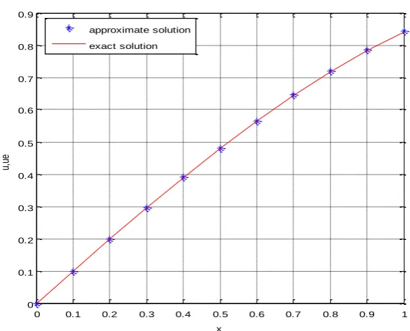
Fig.1 Exact solution and numerical solution for
0 0.1 0.2 0.3 0.4 0.5 0.6 0.7 0.8 0.9 1
0 0.1 0.2 0.3 0.4 0.5 0.6 0.7 0.8 0.9
x
u
,u
e
TABLE II
COMPUTED EXACT, APPROXIMATE SOLUTION AND ABSOLUTE ERROR FOR
Exact Solution Approximate
Solution Error
0 0 0 0.00E+00
0.1 0.099833416646828 0.100000000000000 1.67E-04 0.2 0.198669330795061 0.199000000000000 3.31E-04 0.3 0.295520206661340 0.296010000000000 4.90E-04 0.4 0.389418342308651 0.390059900000000 6.42E-04 0.5 0.479425538604203 0.480209201000000 7.84E-04 0.6 0.564642473395035 0.565556409990000 9.14E-04 0.7 0.644217687237691 0.645248054880100 1.03E-03 0.8 0.717356090899523 0.718487219221399 1.13E-03 0.9 0.783326909627483 0.784541511370484 1.21E-03 1.0 0.841470984807897 0.842750388405864 1.28E-03
Fig.2 Exact solution and numerical solution for
0 0.1 0.2 0.3 0.4 0.5 0.6 0.7 0.8 0.9 1
0 0.1 0.2 0.3 0.4 0.5 0.6 0.7 0.8 0.9
x
u,
ue
TABLE III
COMPUTED EXACT, APPROXIMATE SOLUTION AND ABSOLUTE ERROR FOR
ABLE II
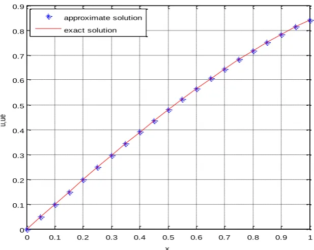
Fig.3 Exact solution and numerical solution for
Exact Solution Approximate
Solution Error
0 0 0 0.00E+00
0.05 0.049979169270678 0.050000000000000 2.08E-05 0.10 0.099833416646828 0.099875000000000 4.16E-05 0.15 0.149438132473599 0.149500312500000 6.22E-05 0.20 0.198669330795061 0.198751874218750 8.25E-05 0.25 0.247403959254523 0.247506556251953 1.03E-04 0.30 0.295520206661340 0.295642471894526 1.22E-04
0.35 0.342897807455451 0.343039281357363 1.41E-04 0.40 0.389418342308651 0.389578492616807 1.60E-04 0.45 0.434965534111230 0.435143757644708 1.78E-04
0.50 0.479425538604203 0.479621163278498 1.96E-04 0.55 0.522687228930659 0.522899516004092 2.12E-04
0.60 0.564642473395035 0.564870619939675 2.28E-04 0.65 0.605186405736040 0.605429547325409 2.43E-04 0.70 0.644217687237691 0.644474900842829 2.57E-04
0.75 0.681638760023334 0.681909067108143 2.70E-04 0.80 0.717356090899523 0.717638460705686 2.82E-04
0.85 0.751280405140293 0.751573758151465 2.93E-04 0.90 0.783326909627483 0.783630121201865 3.03E-04
0.95 0.813415504789374 0.813727408949261 3.12E-04 1.00 0.841470984807897 0.841790378174283 3.19E-04
0 0.1 0.2 0.3 0.4 0.5 0.6 0.7 0.8 0.9 1
0 0.1 0.2 0.3 0.4 0.5 0.6 0.7 0.8 0.9
x
u,
ue
V. CONCLUSIONS
In this paper, a very simple and efficient Trapezoidal method has been developed to solve second kind Volterra integral equations. The numerical results obtained by the proposed method are in good agreement with the exact solutions. In this paper, we may note that the numerical solutions coincide with the exact solutions even a few Numerical Solutions of Volterra Integral Equations of Second kind with the help of Trapezoidal method are used in the approximation, which are shown in the numerical example. We also notice that the accuracy increase with increase the number of interval partitions ( ) in the approximations, which is shown in Table 1, Table 2 and Table 3. We may realize that this method may be applied to solve other integral equations for the desired accuracy.
R
EFERENCES
[1] Abdul J. Jerri, Introduction to Integral Equations with Applications, John Wiley & Sons Inc., (1999). [2] N. Saran, S. D. Sharma and T. N. Trivedi, Special Functions, Seventh edition, Pragati Prakashan, (2000). [3] M. Rahman, Integral equations and their Applications, WITPress, USA (2007).
[4] M. M. Rahman, M . A. Hakim, M. Kamrul Hassan, M. K. Alam and L. Nowsher Ali, Numerical solution of Volterra Integral Equations of second kind with help of Chebyshev polynomials, Annals of Pure and Applied mathematics, Vol. 1, No. 2, (2012), 158-167.
[5] Steven C. Chapra, Applied Numerical Methods with MATLAB for Engineers and Scientists, Second edition, Tata McGraw-Hill, (2007).