Partial Key Exposure Attacks on RSA: Achieving the Boneh-Durfee Bound

(1)

Partial Key Exposure Attacks on RSA:

Achieving the Boneh-Durfee Bound

∗

†_{Atsushi Takayasu and}‡_{Noboru Kunihiro}

May 25, 2018

Abstract

Thus far, several lattice-based algorithms forpartial key exposure attackson RSA, i.e., given the most/least significant bits (MSBs/LSBs) of a secret exponentdand factoring an RSA mod-ulusN, have been proposed such as Bl¨omer and May (Crypto’03), Ernst et al. (Eurocrypt’05), and Aono (PKC’09). Due to Boneh and Durfee’s small secret exponent attack, partial key expo-sure attacks should always work ford < N0.292 _{even without any partial information. However,} it was diﬃcult task to make use of the given partial information without losing the quality of Boneh-Durfee’s attack. In particular, known partial key exposure attacks fail to work for d < N0.292_{with only few partial information. Such unnatural situation stems from the fact that} the additional information makes underlying modular equations involved. In this paper, we pro-pose improved attacks when a secret exponentsdis small. Our attacks are better than all known previous attacks in the sense that our attacks require less partial information. Specifically, our attack is better than all known ones for d < N0.5625 and d < N0.368 with the MSBs and the LSBs, respectively. Furthermore, our attacks fully cover the Boneh-Durfee bound, i.e., they always work ford < N0.292_{. At a high level, we obtain the improved attacks by fully utilizing}

unravelled linearization technique proposed by Herrmann and May (Asiacrypt’09). Although Herrmann and May (PKC’10) already applied the technique to Boneh-Durfee’s attack, we show elegant and impressive extensions to capture partial key exposure attacks. More concretely, we construct structured triangular matrices that enable us to recover more useful algebraic struc-tures of underlying modular polynomials. We embed the given MSBs/LSBs to the recovered algebraic structures and construct our partial key exposure attacks. In this full version, we provide overviews and explicit proofs of the triangular matrix constructions. We believe that the additional explanations help readers to understand our techniques.

∗_{This is the full version of [TK14c].}

†_{The University of Tokyo, National Institute of Advanced Industrial Science and Technology (AIST). e-mail:}

[email protected]

(2)

1 Introduction

1.1 Background

RSA is one of the most famous public key cryptosystems and numerous papers have studied the

security. Let N = pq be a public modulus, where p and q are distinct primes with the same

bit-size. The bit-size of N should be suﬃciently large so that the factorization is computationally

hard. There are a public exponent e and a secret exponent d that satisfy ed = 1 modϕ(N),

whereϕ(N) = (p−1)(q−1) is Euler’s totient function. During decryption/signing, heavy modular

exponentiationscd mod N should be computed. The most trivial way to reduce the computational

cost is using smalld. However, Wiener [Wie90] first reported that too smalldmakes RSA insecure.

He claimed that there is a polynomial time algorithm for factoring N when d < N1/4. Boneh and

Durfee [BD00] revisited the attack by using lattice-based Coppersmith’s method [Cop96b]. At first,

they proposed an improved attack that works for d < N(7−2√7)/6 = N0.284···. In the same work,

they further improved the bound tod < N1−1/√2 =N0.292···. Throughout the paper, we call these

bounds the Boneh-Durfee weaker and the stronger bound, respectively.

Boneh, Durfee, and Frankel [BDF98] introduced partial key exposure attacks on RSA, where

the attackers are given the most/least significant bits (MSBs/LSBs) of full size d. The attack

is theoretically interesting to study how many portions of secret information enable attackers to break the security of RSA. Although Boneh et al.’s partial key exposure attacks work only for small

e, several improvements have been proposed by using Coppersmith’s methods [Cop96a,Cop96b].

Bl¨omer and May [BM03] improved the bound to e < N7/8 with the LSBs of d. Ernst et al.

[EJMdW05] proposed the first attack for full size ewith the MSBs ofd.

In the same work [EJMdW05], Ernst et al. also studied the attacks with the MSBs/LSBs of small d. By definition, the attack scenario is an extension of Boneh-Durfee’s work [BD00]. Specifically, Boneh-Durfee’s small secret exponent attack is a special case of the partial key exposure attack when the given partial information is exactly zero. Hence, Boneh and Durfee’s result suggests that partial

key exposure attacks should always work for d < N0.292··· even without any partial information.

However, Ernst et al.’s attacks only cover the Boneh-Durfee weaker bound d < N0.284··· when the

given partial information is exactly zero. Aono [Aon09] proposed the first attack to cover the

Boneh-Durfee stronger bound with the LSBs of d. Aono’s attack requires less partial information

than Ernst et al.’s attack for d < N(9−√21)/12 =N0.368··· to factor a modulusN. Unfortunately, a

trick of Aono’s algorithm is not applicable to the MSBs case. Hence, extending the Boneh-Durfee

stronger attack with MSBs ofdis still an interesting open problem.

1.2 Our Results

In this paper, we propose improved partial key exposure attacks on RSA with the MSBs/LSBs

of d. Our attacks work with less partial information than the previous attacks [Aon09, BM03,

EJMdW05, SSM10] for d < N9/16 = N0.5625 and d < N(9−√21)/12 = N0.368··· with the MSBs

and the LSBs, respectively. Furthermore, the most impressive feature of our proposed attacks is

that they always work for d < N0.292··· even when the given partial information is exactly zero.

(4)

0 0.1 0.2 0.3 0.4 0.5 0.6 0.7

0.3 0.35 0.4 0.45 0.5 0.55

(

)

/

<latexit sha1_base64="0c5NwzOcfwdlSkA7lmD896Alg40=">AAACeXichVHLSsNAFD2N7/pofSwEN2pRqmC9UUFxJbpxWR9VwUpJ0lFD0yQk04IWf8AfcOFGBRH1M9z4Ay76CeJSwYUuvE0DoqLekJlzz9xz58yM7lqmL4mqEaWhsam5pbUt2t7R2RWLd/ds+E7JM0TGcCzH29I1X1imLTLSlJbYcj2hFXVLbOqFpdr6Zll4vunY6/LAFTtFbc82d01Dk0zl4n3JrC6kNpHNC0tqY5NBlosnKEVBDP4EaggSCCPtxK+QRR4ODJRQhIANydiCBp+/bagguMztoMKcx8gM1gWOEGVtiasEV2jMFnjc42w7ZG3Oaz39QG3wLhb/HisHMUIPdE3PdE+39Ejvv/aqBD1qXg541uta4eZix/1rr/+qijxL7H+q/vQssYu5wKvJ3t2AqZ3CqOvLhyfPa/OrI5VRuqAn9n9OVbrjE9jlF+NyRayeIsoPoH6/7p9gYyqlUkpdmUksLIZP0YoBDCPJ9z2LBSwjjQzve4gzXOMm8qYMKUllvF6qREJNL76EMv0BnRCRcg==</latexit><latexit sha1_base64="0c5NwzOcfwdlSkA7lmD896Alg40=">AAACeXichVHLSsNAFD2N7/pofSwEN2pRqmC9UUFxJbpxWR9VwUpJ0lFD0yQk04IWf8AfcOFGBRH1M9z4Ay76CeJSwYUuvE0DoqLekJlzz9xz58yM7lqmL4mqEaWhsam5pbUt2t7R2RWLd/ds+E7JM0TGcCzH29I1X1imLTLSlJbYcj2hFXVLbOqFpdr6Zll4vunY6/LAFTtFbc82d01Dk0zl4n3JrC6kNpHNC0tqY5NBlosnKEVBDP4EaggSCCPtxK+QRR4ODJRQhIANydiCBp+/bagguMztoMKcx8gM1gWOEGVtiasEV2jMFnjc42w7ZG3Oaz39QG3wLhb/HisHMUIPdE3PdE+39Ejvv/aqBD1qXg541uta4eZix/1rr/+qijxL7H+q/vQssYu5wKvJ3t2AqZ3CqOvLhyfPa/OrI5VRuqAn9n9OVbrjE9jlF+NyRayeIsoPoH6/7p9gYyqlUkpdmUksLIZP0YoBDCPJ9z2LBSwjjQzve4gzXOMm8qYMKUllvF6qREJNL76EMv0BnRCRcg==</latexit>

<latexit sha1_base64="0c5NwzOcfwdlSkA7lmD896Alg40=">AAACeXichVHLSsNAFD2N7/pofSwEN2pRqmC9UUFxJbpxWR9VwUpJ0lFD0yQk04IWf8AfcOFGBRH1M9z4Ay76CeJSwYUuvE0DoqLekJlzz9xz58yM7lqmL4mqEaWhsam5pbUt2t7R2RWLd/ds+E7JM0TGcCzH29I1X1imLTLSlJbYcj2hFXVLbOqFpdr6Zll4vunY6/LAFTtFbc82d01Dk0zl4n3JrC6kNpHNC0tqY5NBlosnKEVBDP4EaggSCCPtxK+QRR4ODJRQhIANydiCBp+/bagguMztoMKcx8gM1gWOEGVtiasEV2jMFnjc42w7ZG3Oaz39QG3wLhb/HisHMUIPdE3PdE+39Ejvv/aqBD1qXg541uta4eZix/1rr/+qijxL7H+q/vQssYu5wKvJ3t2AqZ3CqOvLhyfPa/OrI5VRuqAn9n9OVbrjE9jlF+NyRayeIsoPoH6/7p9gYyqlUkpdmUksLIZP0YoBDCPJ9z2LBSwjjQzve4gzXOMm8qYMKUllvF6qREJNL76EMv0BnRCRcg==</latexit>

<latexit sha1_base64="8Y5XGkcC2kNWQPt7gXv4LujJi+I=">AAACaHichVFNLwNBGH66vuurOCAujYY4Ne+KhDgJF0dtVSU0ze4aTGx3N7vTJjT+gIsj4kQiIn6Giz/g0J+AI4mLg7fbTQTBO5mZZ555n3eemTE9WwaKqB7TWlrb2js6u+LdPb19/YmBwbXArfiWyFuu7frrphEIWzoir6SyxbrnC6Ns2qJg7i019gtV4QfSdVbVvieKZWPHkdvSMhRT+U1TKKOUSFGawkj+BHoEUohixU1cYxNbcGGhgjIEHCjGNgwE3Dagg+AxV0SNOZ+RDPcFDhFnbYWzBGcYzO7xuMOrjYh1eN2oGYRqi0+xufusTGKCHuiGXuiebumR3n+tVQtrNLzs82w2tcIr9R+N5N7+VZV5Vtj9VP3pWWEbc6FXyd69kGncwmrqqwcnL7n57ERtki7pmf1fUJ3u+AZO9dW6yojsOeL8Afr35/4J1qbTOqX1zExqYTH6ik6MYRxT/N6zWMAyVpDncyWOcYqz2JOW0Ia10WaqFos0Q/gS2vgHj+iLoA==</latexit>

[EJMdW05]

0 0.05 0.1 0.15 0.2 0.25 0.3 0.35 0.4

0.28 0.29 0.3 0.31 0.32 0.33 0.34 0.35 0.36 0.37

<latexit sha1_base64="8Y5XGkcC2kNWQPt7gXv4LujJi+I=">AAACaHichVFNLwNBGH66vuurOCAujYY4Ne+KhDgJF0dtVSU0ze4aTGx3N7vTJjT+gIsj4kQiIn6Giz/g0J+AI4mLg7fbTQTBO5mZZ555n3eemTE9WwaKqB7TWlrb2js6u+LdPb19/YmBwbXArfiWyFuu7frrphEIWzoir6SyxbrnC6Ns2qJg7i019gtV4QfSdVbVvieKZWPHkdvSMhRT+U1TKKOUSFGawkj+BHoEUohixU1cYxNbcGGhgjIEHCjGNgwE3Dagg+AxV0SNOZ+RDPcFDhFnbYWzBGcYzO7xuMOrjYh1eN2oGYRqi0+xufusTGKCHuiGXuiebumR3n+tVQtrNLzs82w2tcIr9R+N5N7+VZV5Vtj9VP3pWWEbc6FXyd69kGncwmrqqwcnL7n57ERtki7pmf1fUJ3u+AZO9dW6yojsOeL8Afr35/4J1qbTOqX1zExqYTH6ik6MYRxT/N6zWMAyVpDncyWOcYqz2JOW0Ia10WaqFos0Q/gS2vgHj+iLoA==</latexit>

(

)

/

<latexit sha1_base64="0c5NwzOcfwdlSkA7lmD896Alg40=">AAACeXichVHLSsNAFD2N7/pofSwEN2pRqmC9UUFxJbpxWR9VwUpJ0lFD0yQk04IWf8AfcOFGBRH1M9z4Ay76CeJSwYUuvE0DoqLekJlzz9xz58yM7lqmL4mqEaWhsam5pbUt2t7R2RWLd/ds+E7JM0TGcCzH29I1X1imLTLSlJbYcj2hFXVLbOqFpdr6Zll4vunY6/LAFTtFbc82d01Dk0zl4n3JrC6kNpHNC0tqY5NBlosnKEVBDP4EaggSCCPtxK+QRR4ODJRQhIANydiCBp+/bagguMztoMKcx8gM1gWOEGVtiasEV2jMFnjc42w7ZG3Oaz39QG3wLhb/HisHMUIPdE3PdE+39Ejvv/aqBD1qXg541uta4eZix/1rr/+qijxL7H+q/vQssYu5wKvJ3t2AqZ3CqOvLhyfPa/OrI5VRuqAn9n9OVbrjE9jlF+NyRayeIsoPoH6/7p9gYyqlUkpdmUksLIZP0YoBDCPJ9z2LBSwjjQzve4gzXOMm8qYMKUllvF6qREJNL76EMv0BnRCRcg==</latexit>

[EJMdW05]

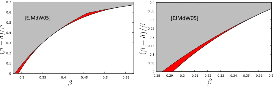
Figure 1: Comparison of attack conditions

Figure 1 compares attack conditions with Ernst et al’s and ours. Since a condition of Aono’s

attack is close to ours, we do not compare it in the figure. The left and the right figure is for the MSBs and the LSBs, respectively. Horizontal axes and vertical axes represent sizes of secret

exponents β := log_Nd and ratios of exposed bits (β−δ)/β, whereδ represents sizes of d1 which

are unknown parts ofd, respectively. Ernst et al.’s attacks work in the gray areas while our attack

improve the red areas whenβ is small.

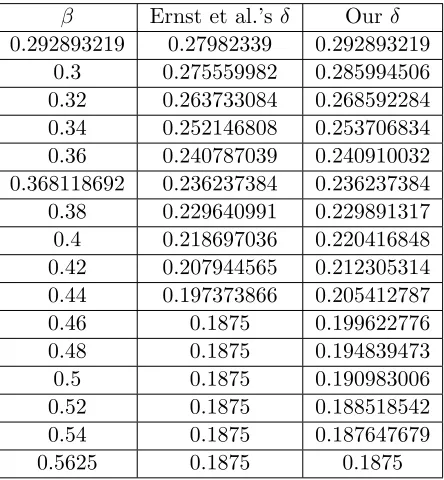
We also show numerical comparisons for attack conditions. Table 1 provides a comparison

between Ernst et al.’s attack and our attack with the MSBs for 1−1/√2 = 0.292· · · ≤β ≤9/16 =

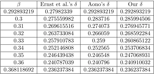
0.5625. Table2 provides a comparison between Ernst et al.’s attack, Aono’s attack, and our attack

for 1−1/√2 = 0.292· · · ≤ β ≤(9−√21)/12 = 0.368· · ·. In such small β, our proposed attacks

are better than other ones.

1.3 Technical Overview

Here, we summarize technical background of the work. Then, we explain a technical overview of our improvements.

Coppersmith’s Methods. In 1996, Coppersmith [Cop96a, Cop96b] introduced lattice-based

methods for solving integer/modular equations with small solutions in polynomial time. The meth-ods first construct a matrix whose rows consist of coeﬃcient vectors of polynomials that have the same roots as the original polynomials. Then, we apply the LLL reduction algorithm [LLL82] to the matrix. If the LLL outputs suﬃciently short vectors, one can obtain the desired solutions. The methods are actively utilized to study the security of RSA including Boneh and Durfee’s small secret

exponent attack [BD00], and partial key exposure attacks [Aon09,BM03,EJMdW05,SSM10].

Some researchers believe that if there is an attack based on Coppersmith’s integer equation solving method, there should be an analogous attack based on the modular equation solving method,

and vice versa. For example, Bl¨omer-May’s [BM03] and Ernst et al.’s [EJMdW05] partial key

(5)

Table 1: Comparison of the recoverable bounds for partial key exposure attacks with the MSBs

β Ernst et al.’s δ Ourδ

0.292893219 0.27982339 0.292893219

0.3 0.275559982 0.285994506

0.32 0.263733084 0.268592284

0.34 0.252146808 0.253706834

0.36 0.240787039 0.240910032

0.368118692 0.236237384 0.236237384

0.38 0.229640991 0.229891317

0.4 0.218697036 0.220416848

0.42 0.207944565 0.212305314

0.44 0.197373866 0.205412787

0.46 0.1875 0.199622776

0.48 0.1875 0.194839473

0.5 0.1875 0.190983006

0.52 0.1875 0.188518542

0.54 0.1875 0.187647679

0.5625 0.1875 0.1875

there are several counterexamples. The most basic example is Boneh-Durfee’s attack [BD00]. Boneh and Durfee utilized Coppersmith’s modular equation solving method to construct their attack. After the proposal, numerous papers have studied several variants of the attack. Then, integer

equation solving analogue has been reported for the Boneh-Durfee weaker bound d < N0.284···.

However, such analogue has not been reported for the stronger boundd < N0.292···.

Due to the situation, solving modular equations seems an appropriate approach to construct partial key exposure attacks that cover the Boneh-Durfee stronger bound. Indeed, Aono [Aon09] took the approach and obtained the desired attack with the LSBs. Hence, Sarkar et al. [SSM10] tried to improve partial key exposure attacks with the MSBs by solving modular equations. However,

what they obtained is the same attack condition as Ernst et al. for N235/512 = N0.458··· ≤ d ≤

N11/16=N0.6875.

Unraveled Linearization. As we claimed above, Coppersmith’s methods can solve modular

equa-tions whose soluequa-tions are small in polynomial time. Constructing partial key exposure attacks with less partial information is equivalent to constructing modular equation solving algorithms that can find larger solutions. Technically, it is further equivalent to constructing basis matrices such that lattices spanned by the matrices have shorter vectors. How to construct such matrices is the most technical part in this research area. To resolve the technical issue, Jochemsz and May [JM06] intro-duced a strategy for the matrix construction. Since the strategy is easy to understand, most works

follow it including partial key exposure attacks of Bl¨omer-May [BM03], Ernst et al. [EJMdW05],

(6)

Table 2: Comparison of the recoverable bounds for partial key exposure attacks with the LSBs

β Ernst et al.’sδ Aono’sδ Our δ

0.292893219 0.27982339 0.292893219 0.292893219

0.3 0.275559982 0.283716 0.285994506

0.31 0.269615516 0.274073 0.276945771

0.32 0.263733084 0.266059 0.268592284

0.33 0.257910783 0.259 0.260865122

0.34 0.252146808 0.252565 0.253706834

0.35 0.246439438 0.246548 0.247068931

0.36 0.240787039 0.240796 0.240910032

0.368118692 0.236237384 0.236237384 0.236237384

always enables ones to construct optimal algorithms. For example, by following the strategy, we obtain the Boneh-Durfee weaker attack. Constructing the stronger one requires a more technical matrix construction. Matrices obtained by the Jochemsz-May strategy are always triangular. Since computing determinants of large matrices is essential task to obtain attack conditions of modular equation solving algorithms, triangular ones simplify the analyses. However, Boneh and Durfee constructed non-triangular matrices to obtain the stronger bound with highly technical analyses.

Due to the fact, there were several attacks [Aon13, DN00, Sar14, Sar16] that are extensions of

Boneh-Durfee’s attack, however, cover only the weaker attack.

In 2009, Herrmann and May [HM09] introduced a novel technique which they called unraveled

linearization. They aimed at introducing the technique to solve nonlinear modular equations.

For the purpose, the technique first applies linearization and obtain new linearized variables; the

linearization combines several monomials into one monomial. Although the linearization has been already taken by numerous papers, the unraveled linearization technique has an additional trick. Reducing the number of monomials has benefit in general, however, the linearization may lose some algebraic information. Hence, during the matrix construction, the technique also applies

unravelingthat cancels the linearization and separates the combined monomials as they were. The

unraveling enables ones to recover the lost algebraic structures. In other words, the unraveled linearization transforms non-triangular basis matrices to triangular ones. Furthermore, if we can apply appropriate unraveling, the matrices preserve useful algebraic structures. Indeed, Herrmann and May [HM10] provided a simpler proof of the Boneh-Durfee stronger attack. After the proposal, the unraveled linearization technique has been intensively utilized to improve several lattice-based

attacks on RSA [BVZ12, Her11, HM10, HHX14, Kun12, KSI14, TK14b, TK14c,TK16a,TK16c,

TK17a,TK17b].

Our Approach. In this paper, we fully utilize the unraveled linearization technique and improve

partial key exposure attacks with the MSBs/LSBs of dby solving modular equations. In this full

(7)

it enables readers to easily understand our subsequent matrix constructions of partial key exposure attacks. In the proof, we apply additional unraveling to Herrmann-May’s triangular matrix while the matrix is still triangular. It means that our triangular matrix recovers lost algebraic structures from Herrmann-May’s one. Although the recovered algebraic structures do not aﬀect the attack condition of the Boneh-Durfee, they are useful for partial key exposure attacks. Specifically, the

recovered structures will enable us to embed the partial information of d.

We provide an improved partial key exposure attack with the MSBs of d by solving modular

equations. As we claimed above, Sarkar et al.’s attack [SSM10] is a modular equation solving

analogue of Ernst et al.’s attack [EJMdW05] forN0.458···≤d≤N0.6875. In this full version, before

providing our improved attack, we first construct modular equation solving analogue of Ernst et

al.’s attack forN0.284···≤d≤N0.458···. The analogous attack can be viewed as an extension of the

Boneh-Durfee weaker attack that utilize the given MSBs of d. We believe that the attack helps

readers to understand how to embed the partial information in Boneh-Durfee’s matrix. Then, we provide our main attack that can be viewed as an extension of the Boneh-Durfee stronger attack with the partial information. We construct the attack by embedding the partial information in Boneh-Durfee’s stronger matrix with additional unraveling. To this end, our additional unraveling becomes eﬀective. Herrmann-May’s matrix does not preserve enough algebraic structures to embed the given partial information. On the other hand, by applying additional unraveling, we recovered lost algebraic structures that are useful to embed the partial information. As a result, we can successfully construct the partial key exposure attack that is an extension of the Boneh-Durfee stronger attack.

Next, we provide an improved partial key exposure attack with the LSBs ofdby solving modular

equations. As we suggested above, Bl¨omer-May’s attack [BM03] works for the same condition

as Ernst et al.’s attack [EJMdW05] and it can be viewed as an extension of the Boneh-Durfee

weaker attack that utilized the given LSBs of d. Hence, the result tells us how to embed the

given partial information in Boneh-Durfee’s weaker matrix. To improve the attack, Aono [Aon09]

constructed a matrix that has two layers. The first layer is the same as Bl¨omer-May’s matrix while

the second layer is the same as Boneh-Durfee’s stronger matrix. The second layer did not utilize

the partial information at all, however, it was eﬀective to improve Bl¨omer-May’s attack. Although

Aono analyzed non-triangular basis matrices, we can obtain the same attack condition by using Herrmann-May’s matrix, which does not have much algebraic structures to embed the given partial information, in the second layer. In our attack, we construct a matrix, where the second layer is replaced by Boneh-Durfee’s stronger matrix with additional unraveling. Since the matrix has more algebraic structures to embed partial information than Aono’s one, we can successfully improve the attack.

1.4 Related Works

Boneh-Dufee’s small secret exponent attack [BD00] is one of the most famous application of

Cop-persmith’s methods [Cop96a, Cop96b]. Thus far, several variants of the attack has been

pro-posed. They include attacks on RSA variants, e.g., unbalanced RSA [DN00, TK16d], prime

power RSA [LZPL15,Sar14, Sar16, TK16a], Takagi’s RSA [IKK08, IKK09,TK16a], multi-prime

(8)

exten-sions [Kun11, Kun12, KSI14, TK17a]. Recently, Aono et al. [AASW18] found an optimality of the Boneh-Durfee stronger attack under heuristic assumptions. As similar settings, there are small CRT exponent attacks [TLP17]. Similarly, there are several partial key exposure on RSA variants,

e.g., prime power RSA [LZPL15,TK16a], Takagi’s RSA [TK16a], multi-prime RSA [Hin08,TK17b],

and RSA with multiple exponent pairs [TK14b,TK16c]. As similar settings, several papers study

partial key exposure attacks on CRT-RSA [SM09,LZL14,TK15,TK16b].

1.5 Roadmap

The organization of this paper is as follows. In Section2, we recall basic tools and an overview of

Coppersmith’s methods to solve modular equations. In Section 3, we provide an alternative proof

of the Boneh-Durfee stronger attack. In Sections 4 and 5, we study partial key exposure attacks

with the MSBs and the LSBs, respectively.

2 Preliminaries

In this section, we recall Coppersmith’s method to solve modular equations with small solu-tions [Cop96b]. Coppersmith’s method has been utilized to reveal several vulnerabilities of RSA.

See [Cop97,Cop01,May03,May10,NS01] for more information. In this paper, we use

Howgrave-Graham’s simpler reformulation of the method [How97]. At the end of the section, we summarize a basic approach to maximize solvable root bounds by utilizing a notion of helpful

polynomi-als [May10,TK14a].

For bivariate polynomialsh(x, y) =∑hi_X,iYx

iX_yiY_{, let}∥_{h(x, y)}∥_:=√∑_h2

iX,iY denote a norm

of the polynomial. The following Howgrave-Graham’s lemma [How97] enables us to solve modular equations by solving integer equations.

Lemma 1 (Howgrave-Graham’s lemma [How97]). Let h(x, y)∈Z[x, y]be a bivariate integer

poly-nomial that consists of at most n monomials. Let W, X, Y be positive integers. If the polynomial

h(x, y) satisfies

1. h(˜x,y) = 0 (mod˜ W), where |x˜|< X,|y˜|< Y,

2. ∥h(xX, yY)∥< W/√n.

Then h(˜x,y) = 0˜ holds over the integers.

Based on the lemma, solving bivariate modular equations is reduced to finding two low norm polynomials that has the same small solutions. To find the polynomials, we utilize the LLL

lat-tice reduction algorithm [LLL82]. Let b1, . . . ,bn be linearly independent k-dimensional vectors.

The lattice L(b1, . . . ,bn) spanned by the basis vectors b1, . . . ,bn is defined as L(b1, . . . ,bn) =

{∑n

j=1cjbj : cj ∈ Z}. When n = k, lattices are described as full rank. The basis matrix of the

lattice B is defined as the n×k matrix that has a basis vector b1, . . . ,bn in each row. In this

paper, we use only full rank lattices, i.e.,k=n. The determinant of a full rank lattice is computed

by vol(L(B)) = |det(B)|. A lattice has infinitely many bases. Finding a basis that contains low

norm vectors is a fundamental lattice problem. The LLL algorithm proposed by Lenstra, Lenstra

(9)

Proposition 1 (LLL algorithm [LLL82, May03]). Given k-dimensional basis vectors b1, . . . ,bn,

the LLL algorithm finds linearly independent lattice vectors v1 and v2 in L(b1, . . . ,bn) such that

∥v1∥ ≤2(n−1)/4(vol(L(B)))1/n and ∥v2∥ ≤2n/2(vol(L(B)))1/(n−1).

These norms are Euclidean norms. The running time is polynomial in k, n, and the maximum

input length of B.

We summarize how Coppersmith’s method finds a solution (˜x,y) of a bivariate modular equation˜

h(x, y) = 0 (modW) if |x˜| < X,|y˜|< Y. At first, we create n polynomialsh1(x, y), . . . , hn(x, y)

that have the root (˜x,y) modulo˜ Wmfor a positive integerm, and so do any integer linear

combina-tions ofh1(x, y), . . . , hn(x, y). Then, we generate basis vectorsb1, . . . ,bnthat are coeﬃcient vectors

of h1(xX, yY), . . . , hn(xX, yY), respectively. All lattice points correspond to polynomials that are

integer linear combinations of h1(x, y), . . . , hn(x, y). Hence, applying the LLL algorithm to B, we

obtain two short vectors v1 and v2 along with their corresponding low norm polynomials ˜h1(x, y)

and ˜h2(x, y). If norms of the polynomials are enough small to satisfy Howgrave-Graham’s lemma,

they have the root (˜x,y) over the integers. The root can eﬃciently be recovered by computing the˜

Gr¨obner bases or resultants of the polynomials. The method is heuristic for the bivariate case since

the polynomials ˜h1(x, y) and ˜h2(x, y) have no assurance of algebraic independency. In this paper,

we assume that these polynomials are algebraic independent and the resultant will not vanish. This assumption should be reasonable since few negative cases have been reported.

To conclude this section, we briefly explain how to construct a better matrix to find larger

solutions. By using Coppersmith’s method, we can recover the root when |det(B)|1/n < Wm by

omitting small terms. Hence, we can recover larger solutions if we can construct a matrix B with

smaller |det(B)|1/n for a fixed m. Since matrices B usually tend to be triangular, |det(B)|1/n

is an absolute value of a geometric mean of all diagonals. Thus, May [May10] defined a notion

of helpful polynomials whose diagonals in B has smaller absolute values than the modulus Wm

since such polynomials reduce the quantity of |det(B)|1/n and contribute to recovering larger

solutions. Indeed, Takayasu and Kunihiro [TK14a] constructed matrices by collecting as many helpful polynomials as possible and as few unhelpful polynomials as possible, then improve several algorithms for solving multivariate modular equations.

In this paper, we follow the approach to improve partial key exposure attacks. Furthermore, we extend the definition of helpful to capture special matrices which we will use. Specifically, to recover algebraic structures of modular polynomials, several diagonals of our matrices will change

by adding a new polynomial. Hence, to minimize |det(B)|1/n for fixed m, we use the following

notion.

Definition 1 (Helpful Polynomials). Let B be a matrix to solve a modular equation h(x, y) = 0

(modW). Let B′ be a matrix that has the same polynomials as B except h′(x, y) and does not

have further polynomials. We call h′(x, y) a helpful polynomial if and only if

det(B′)

det(B) ≤W

m

(10)

3 Revisiting Herrmann-May’s Matrix

In this section, we recall Herrmann-May’s triangular matrix that provides a simpler proof for the Boneh-Durfee stronger attack. Then, we provide an alternative triangular matrix with additional unraveling. Although our matrix does not improve Boneh-Durfee’s attack at all, it will recover useful algebraic structures that will be essential to improve partial key exposure attacks in the subsequent sections.

3.1 Boneh-Durfee’s Attack

We first review the Boneh-Durfee weaker attack. Then, we explain how Boneh-Durfee improves it to the stronger attack.

Recall an RSA key generation

ed= 1 +ℓ(p−1)(q−1) = 1 +ℓ(N −p−q+ 1),

whereℓ is an unknown integer. Boneh and Durfee [BD00] solved the following modular equation

fBD(x, y) := 1 +x(N +y) = 0 (mode)

whose solution is (x, y) = (ℓ,−p−q+ 1). Let ebe full size andd=Nβ. Then, an absolute value of

the solution is bounded above by X := Nβ and Y := N1/2 within a constant factor, respectively.

To recover the solution, Boneh and Durfee utilized the following shift-polynomials

g_[u,i]BD.x(x, y) :=xu−ifBD(x, y)iem−i and g_[u,j]BD.y(x, y) :=yjfBD(x, y)uem−u. (1)

They first defined sets of indices

IBD,x:={u= 0,1, . . . , m;i= 0,1, . . . , u},

IBD,y1:={u= 0,1, . . . , m;j = 1,2, . . . , k}, (2)

where κ = k/m ≥ 0 is a parameter to be optimized. They constructed a matrix B that has a

coeﬃcient vector ofgBD.x_[u,i] (xX, yY) for (u, i)∈ IBD,xandgBD.y_[u,j] (xX, yY) for (u, j)∈ IBD,y1 in each

row. Based on the construction, the matrixB becomes triangular as follows.

Lemma 2 (Boneh-Durfee Weaker Matrix [BD00]). Let shift-polynomials g_[u,i]BD.x(x, y) and

gBD.y_[u,j] (x, y), sets of indices IBD,x and IBD,y1, be defined as in (1), (2), respectively. Let B be

a matrix whose rows consist of coeﬃcients of gBD.x_[u,i] (xX, yY) for (u, i)∈ IBD,x and g_[u,j]BD.y(xX, yY)

for (u, j)∈ IBD,y1. If the shift-polynomials are ordered as

• gBD.x_[u,i] (xX, yY)≺g_[u,j]BD.y(xX, yY),

• gBD.x_[u′_,i′_](xX, yY)≺g_[u,i]BD.x(xX, yY) for

(11)

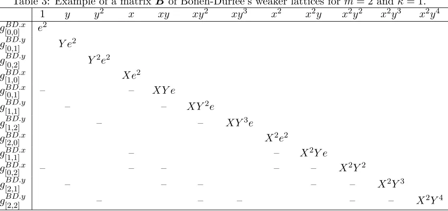
Table 3: Example of a matrixB of Boneh-Durfee’s weaker lattices form= 2 and κ= 1.

1 y y2 _x _xy _xy2 _xy3 _x2 _x2_y _x2_y2 _x2_y3 _x2_y4

g_[0,0]BD.x e2

g_[0,1]BD.y Y e2

g_[0,2]BD.y Y2e2

g_[1,0]BD.x Xe2

g_[0,1]BD.x – – XY e

g_[1,1]BD.y – – XY2e

g_[1,2]BD.y – – XY3e

g_[2,0]BD.x X2e2

g_[1,1]BD.x – – X2Y e

g_[0,2]BD.x – – – – – X2Y2

g_[2,1]BD.y – – – – – X2Y3

g_[2,2]BD.y – – – – – X2Y4

– u′ =u, i′< i,

• gBD.y_[u_′_,j_′_](xX, yY)≺g_[u,j]BD.y(xX, yY) for

– u′ < u,

– u′ =u, j′< j,

then the matrix B becomes triangular with diagonals

• XuYiem−i for gBD.x_[u,i] (xX, yY),

• XuYu+jem−u for g_[u,j]BD.y(xX, yY).

Table3shows1 an example of the triangular matrix. By optimizingκ= (1−2β)/2, the matrix

provides the Boneh-Durfee weaker attack that works whenβ <(7−2√7)/6 = 0.284· · ·.

To improve the weaker attack, Boneh and Durfee exploited sublattices. To be precise, they used a submatrix of the previous one as a lattice basis. For the purpose, they replaced a set of index

IBD,y1 by2

IBD,y2 :={u= 0,1, . . . , m;j= 1,2, . . . , k+⌊τ u⌋}, (3)

1_{“–” in matrices denote non-zero elements throughout the paper.}

2

To be precise, the upper bound ofjinIBD,y2 was⌊τ u⌋in the original paper [BD00]. Indeed, the additionalk

is optimized tok = 0. We modify the upper bound since it will be convenient to explain our partial key exposure

(12)

whereτ is a parameter to be optimized such that 0≤τ ≤1. By optimizingk= 0 andτ = 1−2β,

the matrix B that has a coeﬃcient vector of gBD.x

[u,i] (xX, yY) for (u, i)∈ IBD,x and g

BD.y

[u,j] (xX, yY)

for (u, j) ∈ IBD,y2 in each row provides the Boneh-Durfee stronger attack that works when β <

1−1/√2 = 0.292· · ·. Since the matrix does not become triangular, the analysis is involved.

3.2 Herrmann-May’s Matrix

Herrmann and May [HM10] revisited Boneh-Durfee’s work and provided a simpler proof. Specif-ically, they applied unraveled linearization [HM09] to the Boneh-Durfee’s stronger matrix and transformed it to be triangular. For the purpose, a new variable

z:= 1 +xy

plays an essential role, where an absolute value of the solution is bounded above by Z := XY =

Nβ+1/2within a constant factor. In the following lemma, we summarize Herrmann-May’s triangular

matrix.3

Lemma 3(Herrmann-May’s Triangular Matrix [HM10,TK17a]). Let shift-polynomialsg_[u,i]BD.x(x, y)

and gBD.y_[u,j] (x, y), sets of indices IBD,x and IBD,y2, be defined as in (1), (3), respectively. Let B be

a matrix whose rows consist of coeﬃcients of gBD.x_[u,i] (xX, yY) for (u, i)∈ IBD,x and g_[u,j]BD.y(xX, yY)

for (u, j) ∈ IBD,y2. If the shift-polynomials are ordered as the same way in Lemma 2, then the

matrix B becomes triangular with diagonals

• Xu−i_Zi_em−i _for _gBD.x

[u,i] (xX, yY),

• YjZuem−u for gBD.y_[u,j] (xX, yY).

As the last statement suggests, all monomials do not have two variablesxandy, simultaneously.

Although the linearization z = 1 +xy loses the information of x and y, it can be recovered by

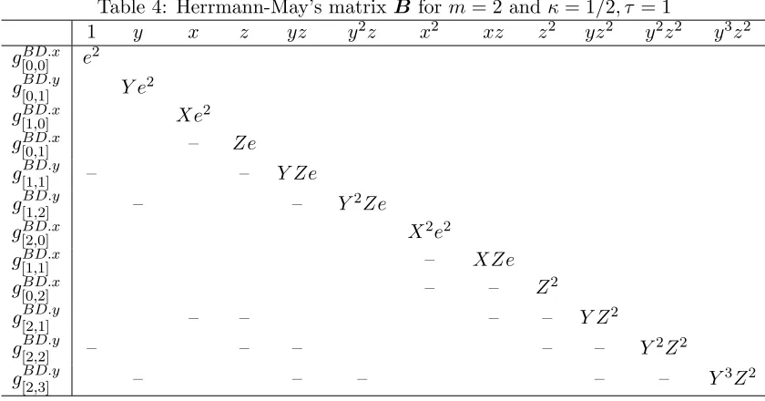
unraveling. Table 4 shows an example of the triangular matrix. The triangular matrix enables us

to analyze the structure easily. Indeed, the following lemma shows one evidence of the optimality of the Boneh-Durfee stronger attack.

Lemma 4. In the matrix B of the Boneh-Durfee stronger attack, polynomials gBD.y_[u,j] (x, y) are

helpful if and only ifj ≤(1−2β)u for all u.

Proof of Lemma 4. Letg_[uBD.y′_,j′_](x, y) be a polynomial with fixed indices (u′, j′), and B′ be a matrix

that is a matrix B without the polynomial gBD.y_[u′_,j′_](x, y). As stated in Lemma3, a diagonal of the

polynomial g_[uBD.y_′_,j_′_](x, y) inB isYj′Zu′em−u′. Hence,

det(B)

det(B′) =Y

j′_Zu′_em−u′

3

As we mentioned, the set of indicesIBD,y2is not the same as the the original one in [BD00]. Hence, it is not the

same as the one which Herrmann and May studied in [HM10]. However, Herrmann-May’s approach is also useful for

(13)

Table 4: Herrmann-May’s matrix B form= 2 andκ= 1/2, τ = 1

1 y x z yz y2z x2 xz z2 yz2 y2z2 y3z2

g_[0,0]BD.x e2

g_[0,1]BD.y Y e2

g_[1,0]BD.x Xe2

g_[0,1]BD.x – Ze

g_[1,1]BD.y – – Y Ze

g_[1,2]BD.y – – Y2Ze

g_[2,0]BD.x X2e2

g_[1,1]BD.x – XZe

g_[0,2]BD.x – – Z2

g_[2,1]BD.y – – – – Y Z2

g_[2,2]BD.y – – – – – Y2Z2

g_[2,3]BD.y – – – – – Y3Z2

that is smaller than or equal to the modulusem _{if and only if}

Yj′Zu′em−u′ ≤em⇔Yj′Zu′ ≤eu′

⇔ 1

2j

′₊(_β₊1

2

)

u′ ≤u′

⇔j′ ≤(1−2β)u′.

Hence, we conclude the proof.

The lemma suggests that the Boneh-Durfee stronger attack used only helpful g_[u,j]BD.y(x, y) and

no unhelpful g_[u,j]BD.y(x, y). That is why they could successfully improve their own weaker attack.

However, we should note that the lemma does not prove a rigorous optimality of the attack.

3.3 Herrmann-May’s Matrix with Additional Unraveling

In this subsection, we show a new triangular matrix for the Boneh-Durfee stronger attack. In short, we apply additional unraveling to Herrmann-May’s triangular matrix. Then, there are several

monomials which have two variables x and y, simultaneously, in our matrix. Before providing the

matrix, we introduce some functions that will be used to control the power of unraveling throughout the paper.

Definition 2. Let m and k be non-negative integers, τ be a real number such that 0 ≤ τ ≤ 1.

(14)

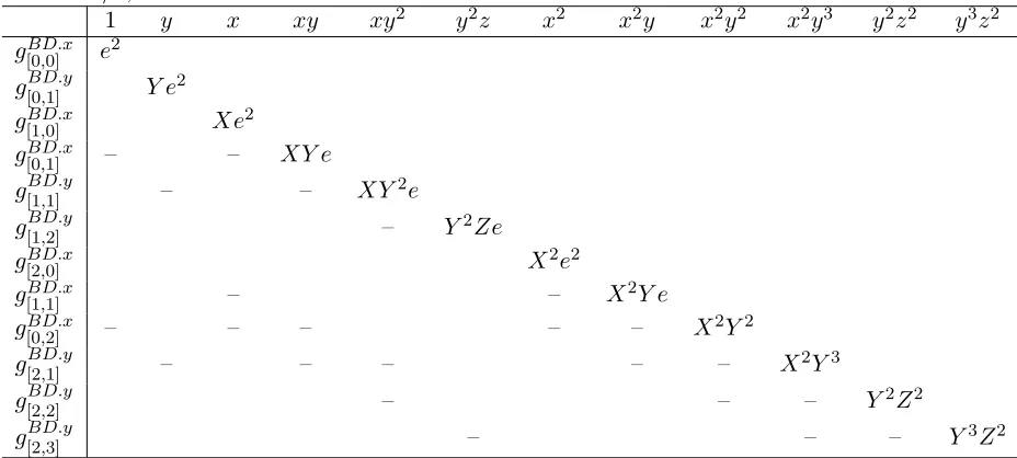
Table 5: Herrmann-May’s matrixB with additional unraveling by the functionlLSBs_k,τ (j) form= 2

and κ= 1/2, τ = 1

1 y x xy xy2 _y2_z _x2 _x2_y _x2_y2 _x2_y3 _y2_z2 _y3_z2

g_[0,0]BD.x e2

g_[0,1]BD.y Y e2

g_[1,0]BD.x Xe2

g_[0,1]BD.x – – XY e

g_[1,1]BD.y – – XY2e

g_[1,2]BD.y – Y2Ze

g_[2,0]BD.x X2e2

g_[1,1]BD.x – – X2Y e

g_[0,2]BD.x – – – – – X2Y2

g_[2,1]BD.y – – – – – X2Y3

g_[2,2]BD.y – – – Y2Z2

g_[2,3]BD.y – – – Y3Z2

integers:

l_k,τM SBs(x) := max

{

0,

⌈

x−k

τ+ 1

⌉}

and l_k,τLSBs(x) := max

{

0,

⌈

x−k

τ

⌉}

.

Then, we provide our matrix.

Lemma 5. Let shift-polynomials g_[u,i]BD.x(x, y) and g_[u,j]BD.y(x, y), sets of indices IBD,x and IBD,y2, a

function lLSBs_k,τ (x), a matrix B be defined as in (1), (3), Definition 2, and Lemma 3, respectively.

If the shift-polynomials are ordered as the same way in Lemma 2, then the matrix B becomes

triangular with diagonals

• XuYiem−i for gBD.x_[u,i] (xX, yY),

• Xu−lLSBsk,τ (j)_Yu+j−lk,τLSBs(j)_ZlLSBsk,τ (j)_em−u _for _gBD.y

[u,j] (xX, yY).

In Herrmann-May’s matrix, two variables x and y does not appear in the same monomials.

Specifically, X does not appear in diagonals ofg_[u,j]BD.y(x, y). However,X appears in our matrix. It

means that we apply less linearizationz= 1 +xy or more unraveling than Herrmann-May’s matrix.

How much we apply linearization/unraveling is controlled by a function lLSBs_k,τ (j).

Table 5 shows an example of the matrix that has the same polynomials as Herrmann-May’s

matrix in Table 4. To illustrate our idea, we use the examples. Herrmann-May’s matrix has

(15)

x2y3 for the same polynomials. We apply additional unravelings z ⇒ 1 +xy and transform the former diagonals to the latter ones by using the following simple relations:

yz =y(1 +xy) =y+xy2 and yz2=y(1 +xy)2 =y+ 2xy2+x2y3.

The relation suggests that all integer linear combinations of (y, yz) and (y, yz, yz2) can be replaced

by those of (y, xy2) and (y, xy2, x2y3), respectively. Hence, the matrix is still triangular even if

we apply the additional unravelings. Here, we want to claim that integer linear combinations of

(yz) and (yz, yz2) cannot be rewritten as those of (xy2) and (xy2, x2y3), respectively. To apply the

additional unraveling, the existence of y was essential. Without the variable y, we cannot replace

yz by xy2. However, since yz exists, we can replaceyz2 by xy2zby using a relation

yz2=yz(1 +xy) =yz+xy2z.

Therefore, we define the function lLSBs_k,τ (j) so that yjzlLSBsk,τ (j) _exists, _however,

yjzlLSBsk,τ (j)−1_{, y}j_zl

LSBs

k,τ (j)−2_,· · · _{do not exist in Herrmann-May’s matrix} _B_. _{In other words,}

in the a set of indicesIBD,y2, there are indices (u, j) = (lLSBs

k,τ (j′), j′),(lk,τLSBs(j′) + 1, j′), . . . ,(m, j′)

whereas no indices (u, j) = (0, j′),(1, j′), . . . ,(lLSBs

k,τ (j′)−1, j′) for a fixed j′ ≥k. The fact follows

from that

• k+⌊τ u⌋< j′ foru < lLSBs

k,τ (j′) since k+⌊τ(lk,τLSBs(j′)−1)⌋< j′ holds,

• k+⌊τ u⌋ ≥j′ foru≥lLSBs_k,τ (j′) since k+⌊τ lLSBs_k,τ (j′)⌋ ≥j′ holds.

Therefore, the functionlLSBs_k,τ (j) tells us the maximum unraveling which we can apply.

The matrix with additional unraveling does not provide any benefits in the context of Boneh-Durfee’s attack. We use the matrix to explain an overview of an unraveled linearization for our

partial key exposure attacks with the LSBs in Section 5.3.

Proof of Lemma 5. We apply unraveling z ⇒ 1 +xy to each variable of Herrmann-May’s

ma-trix B in Lemma 3 and obtain a claimed matrix in Lemma 5. Since the diagonals Xu−iZiem−i

of gBD.x_[u,i] (xX, yY) and those YjZuem−u of g_[u,j]BD.y(xX, yY) for (u, j) = (lLSBs_k,τ (j), j) are the same

between Lemmas3 and 5, we focus on the other variables

• xu−lLSBsk,τ (j)_yu+j−lLSBsk,τ (j)_zlLSBsk,τ (j)_for_j_{= 1,}_{2, . . . , k}₊⌊τ m⌋;_lLSBs

k,τ (j) + 1, , lk,τLSBs(j) + 2, . . . , m.

We want to claim that a matrix B is still triangular when all variables yjzu are replaced by

xu−lk,τLSBs(j)_yu+j−lLSBsk,τ (j)_zlLSBsk,τ (j) _{by applying unraveling}_zu−lLSBsk,τ (j)⇒_{(1 +}_xy)u−lLSBsk,τ (j)_.

Here, we show an inductive proof that

yjzu=

u−lLSBs

k,τ (j) ∑

t=0

(16)

holds, where c0, c1, . . . , cu−lLSBs

k,τ (j) are integers and cu−lLSBsk,τ (j) = 1. The statement holds for u =

lLSBs_k,τ (j). We assume that the statement holds for fixed (u′, j′) and prove that the statement also

holds for (u′+ 1, j′). It follows that

yj′zu′+1 =yj′zu′(1 +xy)

=

  

u′−lLSBs

k,τ∑(j′)

t=0

ctxtyj

′_+t

zlLSBsk,τ (j′)

 

(1 +xy)

=

u′−lLSBs

k,τ (j′) ∑

t=0

ctxtyj

′_+t

zlLSBsk,τ (j′)

+

  

u′−lLSBs

k,τ∑(j′)−1

t=0

ctxtyj′+tzlLSBsk,τ (j′)₊_xu′−lLSBsk,τ (j′)_yu′+j′−lk,τLSBs(j′)_zlLSBsk,τ (j′)

 

xy

=

u′−lLSBs

k,τ (j′) ∑

t=0

c′_txtyj′+tzlLSBsk,τ (j′)₊_xu′−lk,τLSBs(j′)+1_yu′+j′−lk,τLSBs(j′)+1_zlLSBsk,τ (j′)_,

where c′₀, c′₁, . . . , c′_u_′₋_lLSBs

k,τ (j)

are integers. Hence, the statement holds for all (u, j). By

using the relation, we can replace all integer linear combinations of ∑u_u=l′ LSBs

k,τ (j)duy

j_zu

by ∑u_u=l′ LSBs

k,τ (j)d

′

ux

u−lLSBs

k,τ (j)_yu+j−lLSBsk,τ (j)_zlk,τLSBs(j)_, _where _d

lLSBs

k,τ (j), dl LSBs

k,τ (j)+1, . . . , du′ and

d′_lLSBs

k,τ (j)

, d′_lLSBs

k,τ (j)+1

, . . . , d′_u′ are integers such that du′ = d′u′. Thus, we can replace all

vari-ablesyj_zu _{in diagonals of} _gBD.y

[u,j] (x, y) byx

u−lLSBs

k,τ (j)_yu+j−lk,τLSBs(j)_zlLSBsk,τ (j)_{. Hence, we complete the}

proof.

As we claimed, the function lLSBs_k,τ (j) tells us the maximum unraveling which we can apply to

Herrmann-May’s matrixB. On the other hand, Herrmann-May’s matrixB is still triangular when

we apply less additional unraveling than the above one. For example, Herrmann-May’s matrix B

can be modified as a triangular matrix with diagonals

• Xu−lM SBsk,τ (i)_Yi−l M SBs k,τ (i)_Zl

M SBs

k,τ (i)_em−i _for_gBD.x

[u,i] (xX, yY),

• Xu−lM SBsk,τ (u+j)_Yu+j−lk,τM SBs(u+j)_ZlM SBsk,τ (u+j)_em−u _for_gBD.y

[u,j] (xX, yY).

Here, observe that

l_k,τM SBs(u+j) = max

{

0,

⌈

u+j−k

τ+ 1

⌉}

≥max

{

0,

⌈

j−k

τ

⌉}

=lLSBs_k,τ (j)

holds for (u, j) ∈ IBD.y2 since j ≤ k+τ u. Hence, when we apply an unraveling by the function

(17)

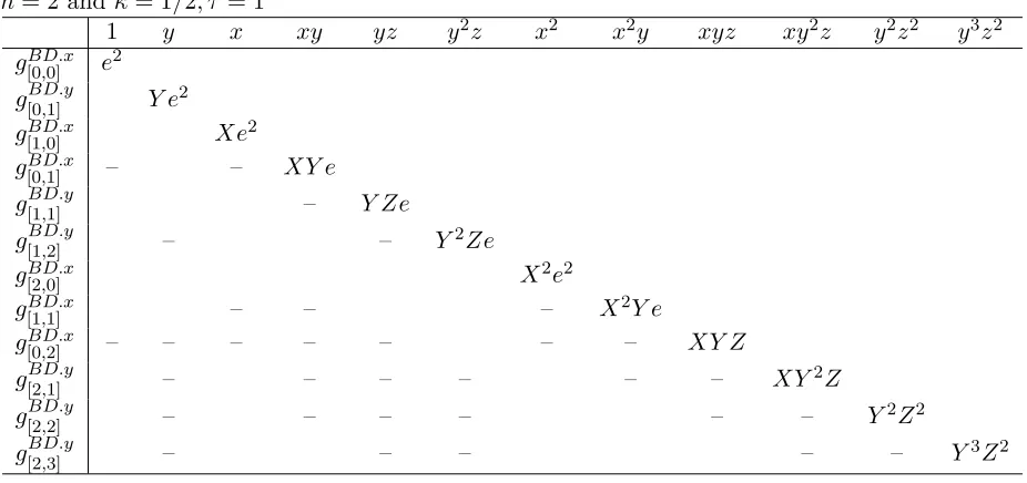
Table 6: Herrmann-May’s matrixB with additional unraveling by the function lM SBs_k,τ (u+j) for

m= 2 and κ= 1/2, τ = 1

1 y x xy yz y2_z _x2 _x2_y _xyz _xy2_z _y2_z2 _y3_z2

g_[0,0]BD.x e2

gBD.y_[0,1] Y e2

g_[1,0]BD.x Xe2

g_[0,1]BD.x – – XY e

gBD.y_[1,1] – Y Ze

gBD.y_[1,2] – – Y2Ze

g_[2,0]BD.x X2e2

g_[1,1]BD.x – – – X2Y e

g_[0,2]BD.x – – – – – – – XY Z

gBD.y_[2,1] – – – – – – XY2Z

gBD.y_[2,2] – – – – – – Y2Z2

gBD.y_[2,3] – – – – – Y3Z2

original matrix and a matrix with an additional unraveling by the function l_k,τLSBs(j). We omit a

proof that a matrix with an unraveling by the function lM SBs

k,τ (u+j) is triangular with the above

diagonals since the proof is almost the same as the that of Lemma5. We use the matrix to explain

an overview of an unraveled linearization for our partial key exposure attacks with the MSBs in

Section4.4.

Table6shows an example of the matrix with an additional unraveling by the functionlM SBs_k,τ (u+

j), where the matrix has the same polynomials as Tables4and5. Herrmann-May’s matrix in Table4

has diagonalsz, xz, z2_,_and_yz2_for_gBD.x

[0,1] , gBD.x[1,1] , gBD.x[0,2] , andg

BD.y

[2,1] whereas our matrix has diagonals

xy, x2_{y, xyz, and} _xy2_z _{for the same polynomials. Our matrix in Table} ₅ _{has diagonals} _xy2_{, x}2_y2_,

and x2y3 for g_[1,1]BD.y, g_[0,2]BD.x, and gBD.y_[2,1] whereas our matrix in Table 6 has diagonals yz, xyz, and

xy2z for the same polynomials.

4 Partial Key Exposure Attacks with the MSBs

In this section, we propose our improved partial key exposure attack on RSA with the MSBs ofd.

In Section 4.1, we formulate the attack scenario as a modular equation. In Section 4.2, we recall

previous attacks [EJMdW05,SSM10]. In Section4.3, we propose an attack that works in the same

condition as Ernst et al.’s attack [EJMdW05] by solving modular equations. In Section 4.4, we

(18)

4.1 Formulation

In this subsection, we formulate the attack scenario with the MSBs as modular equations. We

write a secret exponentd=Nβ asd=d0M+d1, whered0 > Nβ−δandd1< Nδdenote the known

MSBs and the unknown LSBs of d, respectively, with an integer M := 2⌊δlogN⌋. Recall an RSA

key generation

e(d0M +d1) = 1 +ℓ(p−1)(q−1) = 1 +ℓ(N−p−q+ 1) (4)

with an unknown integer ℓas in Section3.1. Let publicly computableℓ0 =⌊(ed0M−1)/N⌋ be an

approximation toℓsince

|ℓ−ℓ0|=e(d0M+d1)−1

N −p−q+ 1 −

⌊

ed0M−1

N

⌋

≤e(d0M+d1)N−N −(ed0M−1)(N−p−q+ 1)

(N−p−q+ 1)N −1

=ed1N−(ed0M−1)(−p−q+ 1)

(N −p−q+ 1)N −1

≤ ed1

N −p−q+ 1

+(ed0M−1)(p+q−1)

(N −p−q+ 1)N

+ 1

≤Nδ+Nβ−1/2+ 1.

Hence, we can bound unknown |ℓ−ℓ0| < Nγ _{such that} _γ _{= max}_{_{δ, β} ₋_1/2_} _{within a constant}

factor. By taking moduloeof the equation (4), we obtain a modular polynomial

fM SBs(x, y) := 1 + (ℓ0+x)(N +y) (mod e)

whose root is (x, y) = (ℓ−ℓ0,−p−q + 1). Absolute values of the root are bounded above by

X:=Nγ andY :=N1/2 within constant factors.

4.2 Previous Works

In this subsection, we briefly recall previous attacks proposed by Ernst et al. [EJMdW05] and Sarkar et al. [SSM10]. Ernst et al.’s attack, which solves integer equations, works when

(1) δ < 5₆ −1₃√1 + 6β,

(2) δ < ₁₆3 and β ≤ 11₁₆,

(3) δ < 1₃ +1₃β−1₃√4β2_{+ 2β}−_{2 and}_{β >} 11

16.

The condition (1) is the best forβ <235/512. Ernst et al.’s attack can be viewed as an extension of

the Boneh-Durfee weaker attack since the condition (1) is the same asβ <(7−2√7)/6 = 0.284· · ·

(19)

Sarkar et al.’s attack, which solves the modular equation fM SBs(x, y) = 0, works in the above condition (2). To solve the modular equation, they used shift-polynomials

g_[u,i]M SBs.x(x, y) :=xu−ifM SBs(x, y)iem−i,

g_[u,j]M SBs.y(x, y) :=yjfM SBs(x, y)uem−u. (5)

Both shift-polynomials modulo em have the same root as the original solutions, i.e., g_[u,i]M SBs.x(ℓ−

ℓ0,−p−q+ 1) = 0 (modem) andg_[u,j]M SBs.y(ℓ−ℓ0,−p−q+ 1) = 0 (modem). They defined sets of

indices

ISSM,x:={u= 0,1, . . . , m;i= 0,1, . . . ,min{u, s}},

ISSM,y :={u= 0,1, . . . , s−1;j= 1,2, . . . , s−u},

and used shift-polynomials gM SBs.x_[u,i] (xX, yY) for (u, i) ∈ ISSM,x and g_[u,j]M SBs.y(xX, yY) for (u, j)∈

ISSM,y to construct a triangular matrix B. The definitions of ISSM,x and ISSM,y quite diﬀers

from Boneh-Durfee’s one although Sarkar et al. solved the similar equation. Indeed, Sarkar et al.’s

attack is not an extension of the Boneh-Durfee attack since it does not work for small d.

4.3 Revisiting Ernst et al.’s Attack by Solving Modular Equations

In this subsection, we show that by solving modular equation fM SBs(x, y) = 0 as Sarkar et al., we

can obtain an attack that works in Ernst et al.’s condition (1). We believe that a content in this

subsection will be useful to understand our improved attacks in Section4.4.

Technically, we use the same shift-polynomials as Sarkar et al., however, we use sets of indices

IBD,xand IBD,y1 as the Boneh-Durfee weaker attack to construct a basis matrixB. Furthermore,

we employ the unraveled linearization to construct triangular matrices. Observe that the modular polynomial

fM SBs(x, y) = 1 + (ℓ0+x)(N+y) (mode)

becomes the same as Boneh-Durfee’s one

fBD(w, y) = 1 +w(N+y) = 0 (mode)

by introducing a linearized variable

w:=ℓ0+x,

where the absolute value of the solution w =ℓ is bounded above by W := Nβ within a constant

factor. Hence, our matrix construction starts from that of the Boneh-Durfee weaker attack in

Section3.1. Then, we partially apply unraveling w=ℓ0+x to utilize the given MSBs.

Proof of the Condition (1) of Ernst et al. As Sarkar et al., we solve the modular equation

fM SBs(x, y) = 0 and use the shift-polynomials g_[u,i]M SBs.x(w, x, y) and g_[u,j]M SBs.y(w, x, y) defined

in (5). As a lattice construction of the Boneh-Durfee weaker attack, we use shift-polynomials

(20)

of indices IBD,x and IBD,y1 were defined in Section 3.1, then construct a basis matrix B. As in

Lemma2, we can construct a triangular matrix if we only use a linearized variablewand do not use

x. To utilize the given partial information and equivalently a variable x, we construct a triangular

matrix as follows.

Lemma 6. Let shift-polynomials g_[u,i]M SBs.x(w, x, y) and g_[u,j]M SBs.y(w, x, y), sets of indices IBD,x and

IBD,y1, a function lM SBs_k,0 (·) be defined as in (5), (2), and Definition 2, respectively. Let B

be a matrix whose rows consist of coeﬃcients of g_[u,i]M SBs.x(wW, xX, yY) for (u, i) ∈ IBD,x and

gM SBs.y_[u,j] (wW, xX, yY) for (u, j)∈ IBD,y1. If the shift-polynomials are ordered as

• gM SBs.x_[u′_,i′_] (wW, xX, yY)≺gM SBs.x_[u,i] (wW, xX, yY) for

– u′ < u,

– u′ =u, i′< i,

• gM SBs.x_[u′_,i′_] (wW, xX, yY)≺gM SBs.y_[u,j] (wW, xX, yY) for u′ ≤u,

• gM SBs.y_[u′_,j′_] (wW, xX, yY)≺g_[u,i]M SBs.x(wW, xX, yY) for u′ < u,

• gM SBs.y_[u′_,j′_] (wW, xX, yY)≺g_[u,j]M SBs.y(wW, xX, yY) for

– u′ < u,

– u′ =u, j′< j′,

then the matrix B becomes triangular with diagonals

• Wlk,M SBs0 (i)_Xu−l M SBs

k,0 (i)_Yi_em−i _for _gM SBs.x

[u,i] (wW, xX, yY),

• Wlk,M SBs0 (u+j)_Xu−lk,M SBs0 (u+j)_Yu+j_em−u _for _gM SBs.y

[u,j] (wW, xX, yY).

If we apply linearizationℓ0+x⇒wto all terms,fM SBs(x, y) =fBD(w, y) holds. Hence, a basis

matrix B is the same as that of the Boneh-Durfee weaker attack in Lemma 2. To utilize partial

information ℓ0, we apply unraveling w⇒ℓ0+x and obtain a matrix as stated in Lemma6. How

much we apply linearization/unraveling is controlled by a function l_k,0M SBs(·).

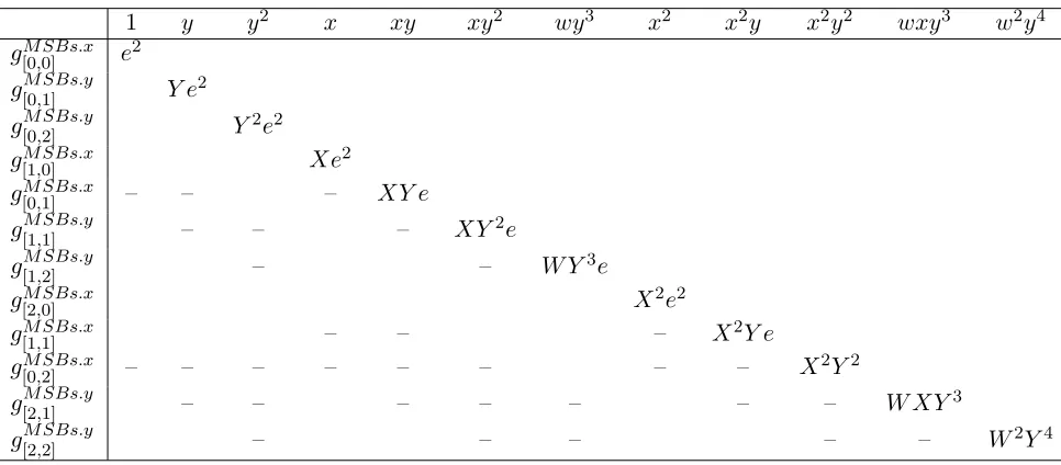
Table 7 shows an example of the matrix that has the same polynomials as Boneh-Durfee’s

weaker matrix in Table 3. To illustrate our idea, we use the examples. Here, please replace a

variable x, a polynomial gBD.x_[u,i] and gBD.y_[u,j] in Table 3 by w, g_[u,i]M SBs.x, and gM SBs.y_[u,j] , respectively,

in mind. Boneh-Durfee’s weaker matrix has diagonals y, wy, and w2y for gM SBs.y_[0,1] , g_[0,1]M SBs.x, and

gM SBs.x

[1,1] whereas our matrix has diagonals y, xy, and x2y for the same polynomials. We apply

unravelings w ⇒ ℓ0+x and transform the former diagonals to the latter diagonals by using the

following simple relations:

Partial Key Exposure Attacks on RSA: Achieving the Boneh-Durfee Bound

Partial Key Exposure Attacks on RSA:

Achieving the Boneh-Durfee Bound

Contents

1

Introduction

(

)

/

2

Preliminaries

3

Revisiting Herrmann-May’s Matrix

4

Partial Key Exposure Attacks with the MSBs