PERFORMANCE EVALUATION FOR GRID ARCHITECTURE

PERFORMANCE EVALUATION FOR GRID

ARCHITECTURE

Nawneet Kumar Pandey

, Raj Kumar Goel

, Ravi Ranjan

ABSTRACT

The parallel computer is one of the remarkable developments of methodology and technology in computer science in recent years. Due to multiprocessor structure of the computer architecture, this computer has a capability to execute multiple instructions or multiple data simultaneously. The parallel computer not only provides support for efficient computation of mathematical, economical, industrial, and ecological problems but also aims new computer architecture beyond the traditional von Neumann type.

In the paper describes the efforts are concentrated on the design of a novel multiprocessor architecture and to schedule the arriving load on to it in order to achieve higher performance. In addition to designing an appropriate network, the efficient management of parallelism on the network involves optimizing performance needed like the minimization of communication and scheduling overhead.

Keywords: Dynamic load balancing, LEC, LET, Hypercube, Gradient model, Debruinju,

Computation delay, Communication delay.

I

INTRODUCTION

One of the most important issues is how to effectively utilized parallel computers that has become increasingly

complex to improve the performance. Such systems are constructed by different processor connected with

communication link to operate in parallel with relatively low cost known as multi processor system.

Multiprocessor system is very efficient at solving problems that can be partitioned into tasks with uniform

computation and communication patterns. However, there exists a large class of non uniform problems with

uneven and unpredictable computation and communication requirements. Therefore Dynamic load balancing

(DLB) schemes are needed to efficiently solve non-uniform problems on multiprocessor systems.

II LITERATURE REVIEW

Achieving Parallelism is now a necessity to improve the performance of computer system. One of the main

Issues is how to effectively utilized parallel computer that has become increasingly complex. It is estimated that

many modern supercomputers and parallel processor deliver only 10 percent or less of their peak performance

potential in a variety of applications. Yet high performance degradation are many. Performance losses occur

because of mismatches among applications software and hardware. Research is active in the direction of

developing new multiprocessor architectures and schedule the partitioned program on to it to achieve higher

Effort concentrated on the Study of all factors for developing a novel multiprocessor Architecture and after

developing we will evaluate the performance of a multiprocessor architecture for server and networking with on

study and to schedule the arriving load on to it in order to achieve higher performance. The other important

issue are accessing delay and downloading the information while using multiprocessor technique. Comparable

with similar architecture. In addition to designing an appropriate network, the efficient management of

parallelism on the network involves optimizing performance needs, like the minimization of communication and

scheduling over head. A simulation studies are carried out to compare the performance of different

multiprocessor architecture (such as LEC, LET, Hypercube, Debruinju etc) with the various standard dynamic

scheduling algorithms like Sender initiated diffusion (SID), receiver initiated diffusion (RID) etc .The

simulation result will show that our Multiprocessor architecture (linearly extensible triangle) gives better

performance as compare to other existing multiprocessor architecture with low cost and reduce the load

balancing time and scheduling over head. Exploiting parallelism is now a necessity to improve the performance

of computer systems one of the most important issues is how to effectively utilize parallel computers that has

become increasingly complex to improve the performance. Such systems are constructed by different processor

connected with communication link to operate in parallel with relatively low cost known as multi processor

system [3,5].

Multiprocessor system is very efficient at solving problems that can be partitioned into tasks with uniform

computation and communication patterns. However, there exists a large class of non uniform problems with

uneven and unpredictable computation and communication requirements. Therefore Dynamic load balancing

(DLB) schemes [1,2,7] are needed to efficiently solve non-uniform problems on multiprocessor systems. Over

the year, much different multiprocessor architecture, having different topological structure and different

interconnection, has been used in different commercially available parallel systems. An enormous amount of

research has centred on the design and their interconnection. Major architecture are found in ring network,

hypercube, debruijn network, LET and LEC network.[3,4,8]. A number of multiprocessor architecture have

been reported in literature.[ 6,7,8] mply with the conference paper formatting requirements is to use this

document as a template and simply type your text into it.

III PROBLEM STATEMENT

Exploiting parallelism is now a necessity to improve the performance of computer systems. In the whole work,

our effort is concentrated on develop a novel multiprocessor architecture with low cost and higher performance.

Schedule the arriving load on it by simulating various scheduling scheme, in order to achieve higher

performance. Compare the performance of proposed network and these scheduling schemes with the standard

hypercube arch and other existing architecture. In addition to designing an appropriate network, the efficient

management of parallelism on the network involves optimizing performance needed like the minimization of

communication and scheduling overhead.

IV DESCRIBING HOW YOU SOLVED THE PROBLEM

 Need of parallelism arise from the need to build faster and faster machines and achieve higher

computing speed.

 When applications require throughput rates that are not easily obtained with today’s sequential

machines, parallel processing offers a solution.

 Parallel processing is based on Multiprocessor processors working together to accomplish a task to

gain high performance.

 Exploiting parallelism is now a necessity to improve the performance of computer systems.

That’s why we need to develop a multiprocessor architecture with low cost and high performance.

Generally stated, parallel processing is based on several processors working together to accomplish a task. The

basic idea is to break down, or partition, the computation into smaller units that are distributed among the

processors. In this way, computation time is reduced by a maximum factor of p, where p is the number of processors present in the multiprocessor system.

Most parallel algorithms incur two basic cost components:

1. Computation delay—under which we subsume all related arithmetic/logic operations, and

2. Communication delay—which includes data movement.

In a realistic analysis, both factors should be considered.

4.2 Existing Multiprocessor Architecture

A processor organization can be represented by a graph in which nodes (Vertices) represent processors and the

edge represent communication paths between pairs of processors.

Figure 1 Figure 2

Hypercube Architecture Debruijn Architecture

Figure 3 Figure4

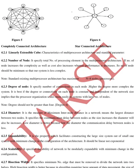
Figure 5 Figure 6

Completely Connected Architecture Star Connected Architecture

4.2.1 Linearly Extensible Cube: Characteristics of multiprocessor architecture and standard parameter:

4.2.2 Number of Node: It specify total No. of processing element in the multiprocessor architecture. If no. of

node increases the complexity as well as cost also increases whereas performance is decreases. So no of node

should be minimum so that our system is less complex.

Note: Standard existing multiprocessor architecture has maximum N=8 nodes (processors).

4.2.3 Degree of node: It specify number of connections in each node .Higher the degree more complex the

system. It is best if the degree or connectivity on each node is constant and independent of the network size

implies that the processor organization scales more easily to systems with large no. of nodes.

Note: Degree should not be greater than four. [Degree 4]

4.2.4 Diameter: It is the measure of Maximum Inter-node distance in a network means the largest distance

between two nodes. It specifies the communication delay between nodes as the size increases the diameter will

also be increases. Low diameter is better because low the diameter the communication delay between nodes is

less.

4.2.5 Expandability: It is the property which facilitates constructing the large size system out of small one

system with minimum change in the configuration of the architecture. It should be linear not exponential

4.2.6 Scalability: It specifies the ability of network to be modularly expandable with minimum change in the

configuration.

4.2.7 Bisection Width: It specifies minimum No. edge that must be removed to divide the network into two

halves. High bisection width is better because in algorithm requiring large amount of data movement, the size of

the data set divided by the bisection width puts a lower bound on the complexity of the parallel system.

4.2.8 Cost: Cost is directly proportional to no. of node in the network. Cost should be minimum as possible as.

4.2.9 Complexity: Complexity is directly proportional to no of node and deg. of node in the network. Less

4.3 Characteristics of Existing Architecture (Comparative study)

V PROPOSED ARCHITECTURE

The proposed architecture named as ―Linearly Extensible Triangle‖ triangular multi- processor network is

simple extensible multiprocessor architecture having different topological properties comparable with existing

architecture.

5.1 Linearly Extensible Triangle

Figure: 7

5.2 Characteristics of Proposed Architecture

No of Node- N=5

Bisection Width- 3

Degree of node- N-1, 3

Diameter- 2

Complexity-Less in comparison to other existing Multi-processor architecture.

Extensibility-Constantly Extensible on each level.

Linearly extensible by Layer of one processor.

5.3 Proposed Performance Parameter

Network No. of Link Node degree. Diameter Bisection Width

Linear Array N-1 2 N-1 1

Star N-1 N-1 2 N-1

Completely Connected N(N-1)/2 N-1 1 (N/2)2 N

Binary Tree N-1 3 2(Log2N -1) 1

Illiac Mesh 2N 4 N -1 2 N

Hypercube NLog2N/2 N Log2N N/2

De-bruijn 2N-1 4 Log2N N/Log2N

To achieve high performance with low cost and minimization of the communication and scheduling overhead

and uniform distribution of load among the processor Standard dynamic scheduling schemes are used namely:

 Hierarchical Balancing method

 Gradient model

 Sender Initiated Diffusion (SID)

5.4 Dynamic load balancing

Dynamic load balancing (DLB) is essential for the efficient use of highly parallel systems when solving

non-uniform problems with unpredictable load estimates. Dynamic load balancing schemes which seek to minimize

total execution time of a single application running in parallel on a multi computer system.

Multi processor system be very efficient at solving problems that can be partitioned into tasks with uniform

computation and communication patterns. However, there exists a large class of non uniform problems with

uneven and unpredictable computation and communication requirements. Therefore Dynamic load balancing

(DLB) schemes are needed to efficiently solve non-uniform problems on multiprocessor systems

To do so, an optimal tradeoff between the processing & communication overhead and the degree of knowledge

used in the balancing process must be sought.

VI A GENERAL DYNAMIC LOAD BALANCING MODEL

We have developed a general model for dynamic load balancing.

This model is organized as a four phase process:

1)Processor load evaluation

2)Load balancing profitability Determination

3)Task migration strategy

4) Task selection strategy

Phase1: Processor Load Evaluation

 A load value is estimated for each processor in the system.

 These values are used as input to the load balancer to detect load imbalances and make load migration

decisions.

Phase2: Load Balancing Profitability Determination

 The imbalance factor quantifies the degree of load imbalance within a processor domain.

 It is used as an estimate of potential speedup obtainable through load balancing

 It is weighed against the load balancing overhead to determine whether or not load balancing is

Phase 3: Task Migration Strategy

Sources and destinations for task migration are determined. Sources are notified of the quantity and destination

of tasks for load balancing.

Phase 4: Task Selection Strategy

Source processors select the most suitable tasks for efficient and effective load balancing and send them to the

appropriate destinations.

 The first and fourth phases of the model are application dependent and purely distributed. Both of these

phases can be executed independently on each individual processor.

 Our focus is on the Profitability Determination and Task Migration phases, the second and third phases,

of the load balancing process

 As the program execution evolves, the inaccuracy of the task requirement estimates leads to

unbalanced load distributions.

 The imbalance must be detected and measured (Phase 2) and an appropriate migration strategy devised

to correct the imbalance (Phase 3).

 During the Profitability Determination Phase a decision is made as to whether or not to invoke the load

balancer.

 The load imbalance factor Ф(t) is an estimate of the potential speedup obtainable through load balancing at time t .

 It is defined as the difference between the maximum processor loads before and after load balancing,

Lmaxand Lbal , respectively.

Ф(t)= Lmax - Lbal

A decision on whether or not to load balance is made based on the value of Ф(t) relative to the balancing overhead, Loverhead, required to perform the load balancing. In general, load balancing is profitable if the savings

is greater than the overhead, i.e.

Ф(t)> Loverhead

The responsibility of invoking the balancer may either be authorized to all processors in the system or only to

designated processors containing the necessary information. For highly parallel systems it is desirable to

distribute the responsibility to multiple points in the system. This may be accomplished by

Partitioning the system into independent groups of processors called balancing domains. The size of a balancing domain may range anywhere from a few processors to the entire system.

Load balancing decisions are based solely on information pertaining to those processors within each domain.

The notion of balancing domains is a way of distributing the balancing process. Furthermore, by decreasing the

number of processors being considered in the balancing process, balancing domains

reduce the complexity of calculating the imbalance factor as well as the complexity of phase 3, the Load Migration Strategy.

The role of the Task Migration Phase is first, to balance the load within each domain by identifying source and

balance the load across the entire system. The concept of balancing domains reduces the overhead of the

balancing process, but does not ensure a balanced load for the entire system. This is accomplished by either

overlapping domains, whereby excess load can diffuse from more heavily loaded domains into lightly loaded

ones, or through the use of variable domains, whereby the set of processors belonging to a domain periodically

changes to encompass a different subset of processors within the system. Potentially more accurate migration

strategies are made possible by larger balancing domains. However, larger domains may increase the aging

period of information and cause the load balancing overhead to be more unevenly distributed. These tradeoffs

are illustrated by the different strategies to be discussed.

VII DYNAMIC LOAD BALANCING STRATEGIES

The following five DLB strategies are designed to support highly parallel systems.

 Sender Initiated Diffusion (SID)

 Receiver Initiated Diffusion (RID)

 Hierarchical Balancing Method (HBM)

 Gradient Model (GM)

 Dimension Exchange Method (DEM)

The schemes presented vary in the amount of processing and communication overhead and in the degree of knowledge used in making balancing decisions.

(1) Knowledge- The accuracy of each balancing decision

(2) Overhead- The amount of added processing and communication incurred by the balancing process.

The load balancing overhead includes the communication costs of acquiring load information and of informing

processors of load migration decisions, and the processing costs of evaluating load information to determine

task transfers. In this work, we use Sender Initiated Diffusion (SID) for performance evaluation our proposed

architecture on the basis of parameter LIF and TIME.

7.1

Sender Initiated Diffusion (SID)

The SID strategy is a, local, near-neighbor diffusion approach which employs overlapping balancing domains to achieve global balancing. A similar strategy, called Neighborhood averaging, is proposed in . The scheme is

purely distributed and asynchronous. Each processor acts independently, apportioning excess load to deficient

neighbors.

It has been shown in, that for an N processor system with a total system load L unevenly distributed across the system, a diffusion approach, such as the SID strategy, will eventually cause each processor’s load to converge

to L/N.

Balancing is performed by each processor whenever it receives a load update message from a neighbor

indicating that the neighbors load, 1i<Ideal Load, where Ideal Load is apreset threshold. Each processor is limited to load information from within its own domain, which consists of itself and its immediate neighbors.

execution. The profitability of load balancing is determined by first computing the average load in the domain,

Lp,

7.2 Receiver Initiated Diffusion (RlD)

The RID strategy can be thought of as the converse of the SID strategy in that it is a receiver initiated approach

as opposed to a sender initiated approach. However, besides the fact that in the RID strategy under loaded

processors request load from overloaded neighbors, certain subtle differences exist between the strategies. First,

the balancing process is initiated by any processor whose load drops below a pre specified threshold ( L L o w ) .

Second, upon receipt of a load request, a processor will fulfill the request only up to an amount equal to half of

its current load (this reduces the effect of the aging of the data upon which the request was based). Finally, in the

receiver initiated approach the underloaded processors in the system take on the majority of the load balancing

overhead, which can be significant when the task granularity is fine.

As with the SID strategy, each processor is limited to load information from within its own domain, which

consists of itself and its immediate neighbors. All processors inform their near-neighbors of their load levels and

update this information throughout program execution.

The RID strategy differs from its counterpart SID in the task migration phase. Here, an underloaded processor

first sends out requests for load and then receives acknowledgment for each request.

7.3 The Gradient Model (GM)

 The gradient model is a demand driven approach .

 The basic concept is that under loaded processors inform other processors in the system of their state,

and overloaded processors respond by sending a portion of their load to the nearest lightly loaded

processor in the system.

 This model employs a gradient map of the proximities of under loaded processors in the system to

guide the migration of tasks between overloaded and under loaded processors.

The resulting effect is a form of relaxation where tasks migrating through the system are guided by the

proximity gradient and gravitate towards underloaded points. The scheme is based on two threshold parameters:

the Low-Water-Mark (LWM) and the High- Water-Mark (HWM). A processor’s state is considered light if its

load is below the LWM, heavy if above the HWM, and moderate otherwise. A node’s proximity is defined as

the shortest distance from itself to the nearest lightly loaded node in the system. All nodes are initialized with a

proximity of wmax, aconstant equal to the diameter of the system. The proximity of a node is set to 0 if its state

becomes light. All other nodes p with near-neighbors n2 computes their proximity as proximity(p) = min (proximity(ni)) + 1.

A node’s proximity may not exceed wmax. A system is saturated, and does not require load balancing if all nodes

report proximity of wmax.If the proximity of a node changes it must notify its near-neighbors. Hence, the

proximities of underloaded processors in the system serves to route tasks between overloaded and underloaded

processors. Load balancing profitability determination is controlled by the LWM and HWM thresholds. In order

for load balancing to take place, there must be at least one overloaded processor and one underloaded processor

in the system. No measure of the degree of imbalance is made, only that one exists. This criterion is

characterized by the simplified version of the load balancing profitability determination phase , where, given an overloaded processor p and an underloaded processor q,

Lp - Lq > HWM - LWM.

The proximity map is used to perform the migration phase. If a processor’s state is heavy and any of its

near-neighbors report a proximity less than wmax, then it sends a unit of its load to the neighbor of lowest proximity. Tasks are routed through the system in the direction of the nearest underloaded processors. A task continues to

migrate until it reaches an underloaded processor or it reaches a node for which no neighboring nodes report a

lower proximity. The scheme is illustrated in Fig. In this example, there are two overloaded nodes in the system

and one under loaded node. The overloaded nodes are at different proximities from the under loaded node, but

both send a fraction of load, 6, in the direction of the under loaded processor. The value of 5 can be determined as either a percentage of the initial load, or as a fixed number of tasks. The scheme may perform inefficiently

when either too much or too little work is sent to an under loaded processor.

7.3.1 GM Complexity: The overhead incurred by the GM strategy includes the updating of the proximity map an the routing of tasks from overloaded processors to under loaded ones. The proximity map is constructed in an

iterative fashion as the existence of an under loaded processor is propagated through the system. The number of

messages required to update the proximity map is dependent on the interconnection network topology, the

number of under loaded processors, their locations, and the order in which they become under loaded. All but

one of these factors is application dependent, making it very difficult to model the complexity. Given N

processors interconnected using a hypercube topology, in the worst case, an update of the gradient map, to

recognize the presence of a new under loaded processor, would require,

CtOt(update) = N log Nmessages.

The worst case occurs when there are no other under loaded processors in the system. Normally, the presence of

other under loaded processors will halt the propagation of update messages to processors closer to the existing

under loaded processors than to the new one.

The migration of tasks from overloaded to under loaded processors incurs added overhead due to the

asynchronous nature of the algorithm. An overloaded processor sends a fixed portion of load in the direction of the nearest under loaded processor. Since the ultimate destination of migrating tasks is not explicitly known,

intermediate processors in the migration path must be interrupted to perform the routing. Furthermore,

Figure 8

The proximity map may change during a task’s migration, altering its destination. This may occur since the

quantity of the imbalances is not known and multiple overloaded processors may send tasks towards the same

destination, creating a migration overflow and a sudden change in the proximity gradient. At the other extreme,

an overloaded processor, in transferring a preset portion of load, may not send enough to solve the imbalance.

Hence, the degree of information used in the balancing process may lead to inefficient migration decisions.

7.4 Hierarchical Balancing Method (HBM)

 Itis an asynchronous global, approach which organizes the system into a hierarchy of subsystems.

 Load balancing is initiated at the lowest levels in the hierarchy with small subsets of processors and

ascends to the highest level which encompasses the entire system.

 Specific processors are designated to control the balancing operations at different levels of the

hierarchy.

Figure 9

 The hierarchical balancing scheme functions asynchronously.

 The balancing process is triggered at different levels in the hierarchy by the receipt of load update

messages indicating an imbalance between lower level domains.

 All load levels are initialized with each processor sending its load information up the tree.

7.5 Dimension Exchange Method (DEM)

 Load balancing is performed in an iterative fashion by ―folding‖ an N processor system into log N

dimensions and balancing one dimension at a time.

Figure 10

 In this scheme small domains are balanced first and these then combine to form larger domains until

ultimately the entire system is balanced.

 In this scheme Balancing is initiated by any underloaded processor which hasa load that drops below a

preset threshold ,

Lp < LThreshold

 This processor broadcasts a load balancing request to all other processors in the system.

7.4.1 DEM Complexity

 In any case, the balancing process is evenly distributed with a total communication overhead :

Ctot = 3N log N (messages).

VIII TESTING & RESULTS (EXPERIMENTAL RESULTS)

In this work, We use Sender Initiated Diffusion (SID) dynamic load balance Strategy for performance

evaluation of our Architecture.

We use two performance parameter for performance evaluation:

1. Load Imbalance Factor (LIF)

2. Load Balancing Time (LBT)

We use four existing multiprocessor architecture for comparative study such as:

1. Linearly Extensible Cube (LEC)

2. Linearly Extensible Tree (LET)

3. Hypercube

4. Debruijn

We use parameter for performance evaluation:

LIF=[(max load on a processor after balancing –Ideal Load)/Ideal Load)]*100

Load Balancing Time= (Time after balancing – Time before balancing)

VIII CONCLUSION AND FUTURE WORK

In this work, we have intended to evaluate the performance of our proposed architecture by comparing other

existing multiprocessor architecture.

So we have use two performance parameter (LIF & LBT). And ―Ideal Load‖ for identifying processor is

overloaded or underloaded. And one scheduling strategy SID (Source Initiated Diffusion) for scheduling or

balancing the arriving the load on processor.

On the basis of above two parameter we have seen that performance of our architecture is better than the other

existing multiprocessor architecture in term of Load Balancing Time and Load Imbalance Factor.

Our architecture has less complexity in terms of interconnection and less processing element in comparison to

other existing multi processor architecture.

So we can say that our proposed architecture( Linearly Extensible Triangle) give better performance in

comparison to other existing multiprocessor architecture.

We are using only one Dynamic Load Balancing Strategies (SID) for simulation study, it can be extended to use

more than one DLB Strategies (Such as RID, Gradient model etc) for comparison and simulation Study.

We use the only two performance parameter (LIF & TIME) for performance evaluation of our proposed

architecture; it can be extended to include other performance parameter of performance evaluation.

We compare our architecture with some existing multiprocessor architecture,

It can be extended to include some more existing multiprocessor architecture.

References:

[1] A.Samad, M.Q. Rafiq and Omar Farooq ―A novel algorithim for fast retrival of information from a

multiprocessor server‖ Proc. Intl. on parallel and distributed system, U.K. Feb 20 to feb 22, 2008

[2] Marc H. Willebeek-LeMair, Member, IEEE, and Anthony P. Reeves ―Strategies for Dynamic Load

Balancing on Highly Parallel Computers‖, Senior Member, IEEE, IEEE TRANSACTIONS ON

PARALLEL AND DISTRIBUTED SYSTEMS, VOL. 4, NO. 9, SEPTEMBER 1993

[3] Z. Zeng and B.Veeravalli ―Design and Performance of Queue and Rate Adjustment Dynamic load Balancing Polices for Distributed Network‖. IEEE trans. On computer, vol 55 ,no. 11, pp. 1410-1422,nov 2006. [4] Abdel A E and Khaled d,‖ The Hyperstar interconnection Network‖journal of Parallel and distributed

computing no. 48,pp 175-199,1998

[5] Razi-Azad H., ―Constraint-based performance comparison of multi-dimensional interconnection networks

with deterministic and adaptive routing strategies‖, Journal of Computers and Electrical Engineering, vol. 30, pp.167-82,2004.

[6] Meraji S., Sarbazi-Azad H., Nayebi A., ―Message routing and performance issues in necklace hypercubes‖,

Technical Report, School of Computer Science, IPM, Tehran,Iran, 2006.

[7] Nizadeh M., and Sarbazi-Azad, H., The necklace hypercube: a well scalable hypercube-based

[8] K. G. Shin and Y.-C. Chang, ―Load sharing in distributed realtime systems with state-change broadcasts,‖

IEEE Trans. Comput., pp. 1124-1142, Aug. 1989.

[9] V. A. Saletore, ―A distrubuted and adaptive dynamic load balancing scheme for parallel processing of

medium-grain tasks,‖ in Proc. Fifth Distributed Memory Comput. Conf, Apr. 1990, pp. 995-999.

[10] W. Shu and L. V. Kale, ―A dynamic scheduling strategy for the Charekernel system,‖ in Proc. ACM Supercomput. Con$, 1989, pp. 389-398.

[11] M. Willebeek-LeMair and A. P. Reeves, ―A general dynamic load balancing model for parallel computers,‖

Tech. Rep. EE-CEG-89- 1,Cornell School of Electrical Engineering, 1989.

[12] T. L. Casavant and J. G. Kuhl, ―A taxonomy of scheduling in generalpurpose distributed computing

systems,‖ IEEE Trans. Software Eng.,vol. 14, no. 2, pp. 141-154, Feb. 1988.

[13] G. Cybenko, ―Dynamic load balancing for distributed memory multiprocessors,‖ J. Parallel and

Distributed Comput., vol. 7:279-301, October, 1989.

[14] D. P. Bertsekas and J. N. Tsitsiklis, Parallel and Distributed Computation:Numerical Methods. Englewood Cliffs, NJ: Prentice-Hall, 1989.K. M. Dragon and J. L. Gustafson,

[15] Aebi A., Sarbazi Azad, H., Shamaei, A., Meraji, S., XMulator: An Object Oriented XML-Based