Article
1
Optimal Network Reconfiguration in Active
2
Distribution Networks with Soft Open Points and
3
Distributed Generation
4
Ibrahim M. Diaaeldin 1, Shady H. E. Abdel Aleem2,*, Ahmed El-Rafei 3, Almoataz Y. Abdelaziz 4
5
and Ahmed F. Zobaa 5,*
6
1 Engineering Physics and Mathematics Department, Ain Shams University, Cairo, Egypt;
7
[email protected]; [email protected]
8
2 Mathematical, Physical and Engineering Sciences Department, 15th of May Higher Institute of
9
Engineering, Cairo, Egypt; [email protected]; [email protected]
10
3 Engineering Physics and Mathematics Department, Ain Shams University, Cairo, Egypt;
11
12
4 Electric Power and Machines Department, Ain Shams University, Cairo, Egypt;
13
[email protected]; [email protected]; [email protected]
14
5 Electronic and Computer Engineering Department, Brunel University London, Uxbridge UB8 3PH, U.K.;
15
16
* Correspondence: [email protected]; Tel.: +2-01227567489
17
18
Abstract: In this paper, a recent meta-heuristic optimization algorithm called the
discrete-19
continuous hyper-spherical search algorithm is used to solve the mixed-integer nonlinear problem
20
of soft open points (SOPs) and renewable distributed generators allocation along with new network
21
reconfiguration methodology under different loading conditions to minimize the total power loss
22
in balanced distribution systems. Multi-scenario studies, which aim to improve the investigation of
23
the overall performance of the strategies, are conducted on IEEE 33-node and 83-node balanced
24
distribution systems. The contributions of SOP losses to the total active losses, as well as the effect
25
of increasing the number of SOPs connected to the system, are investigated to determine the real
26
benefits gained from their allocation. The results obtained validate, with proper justifications, the
27
effectiveness of allocating both SOPs and renewable distributed generators with the proposed
28
network reconfiguration methodology to provide the best operation of distribution networks with
29
minimum losses and enhanced power quality performance. It was also shown that SOPs
30
successfully assist the growing integration plans of the renewable distributed generators units and
31
can address issues related to voltage violations and network losses efficiently.
32
Keywords: Distributed generator, load balancing, network reconfiguration, optimization, power
33
loss minimization, soft open points.
34
Abbreviations:
35
ADN Active distribution network
B2B VSC Back-to-back voltage source converter
BLP Bi-level programming
CB Capacitor bank
D-HSS Discrete hyper-spherical search algorithm
DC-HSS Discrete-continuous HSS algorithm
DG Distributed generation
EA Evolutionary algorithm
ESS Energy storage system
HC Hosting capacity
HSS Hyper-spherical search algorithm
HSA Harmony search algorithm
MHM Modified honeybee mating
MINLP Mixed-integer nonlinear programming
MISOCP Mixed-integer second-order cone programming
NR Network reconfiguration
PF Power factor
PQ Power quality
PSO Particle swarm optimization
SOP Soft open point
SOCP Second-order cone programming
SC Sphere-center
VSC Voltage source converter
VD Voltage deviation
GA Genetic algorithm
Nomenclature:
36
𝐴𝐴𝑙𝑙𝑙𝑙𝑙𝑙𝑙𝑙𝑆𝑆𝑆𝑆𝑆𝑆 Loss coefficient of VSCs
𝐴𝐴𝐴𝐴𝐴𝐴𝐴𝐴 Aggregate voltage deviation index
AP The assigning probability
𝐴𝐴𝑆𝑆𝑆𝑆 Normalized dominance for each SC
𝐴𝐴𝐷𝐷𝐷𝐷𝐷𝐷 Difference of set objective functions for each set of particles and their sphere-center
𝑓𝑓𝑆𝑆𝑆𝑆 Objective function value for each SC
𝑓𝑓𝑝𝑝𝑝𝑝𝑝𝑝𝑝𝑝𝑝𝑝𝑝𝑝𝑙𝑙𝑝𝑝𝑙𝑙𝑙𝑙𝑜𝑜𝑆𝑆𝑆𝑆 Objective function value for each particle assigned to a SC 𝐴𝐴𝑏𝑏 line current flowing in line 𝑏𝑏
𝐴𝐴𝑏𝑏𝑝𝑝𝑝𝑝𝑝𝑝𝑝𝑝𝑟𝑟 Rated line current flowing in line 𝑏𝑏 𝐿𝐿𝐿𝐿𝐴𝐴𝑏𝑏 Load balancing index of line 𝑏𝑏 𝐿𝐿𝐿𝐿𝐴𝐴𝑝𝑝𝑙𝑙𝑝𝑝 Total load balancing index 𝑀𝑀𝑀𝑀𝑥𝑥𝑝𝑝𝑝𝑝𝑝𝑝𝑝𝑝 Maximum number of iterations
𝑀𝑀 Incidence matrix
𝑁𝑁𝑏𝑏𝑝𝑝 Number of lines existing in the distribution network 𝑁𝑁𝑛𝑛 Number of nodes existing in the distribution network
𝑁𝑁𝑜𝑜 Number of feeders
𝑁𝑁𝐷𝐷𝐷𝐷 Number of distributed generators 𝑁𝑁𝑆𝑆𝑆𝑆𝑆𝑆 Number of allocated SOPs 𝑁𝑁𝑝𝑝𝑙𝑙𝑝𝑝 Population size
𝑁𝑁𝑆𝑆𝑆𝑆 Number of sphere-centers
𝑁𝑁𝑛𝑛𝑝𝑝𝑛𝑛𝑝𝑝𝑝𝑝𝑝𝑝 Number of new generated particles
𝑁𝑁 Number of decision variables
OFD Objective function difference
𝑃𝑃𝑟𝑟𝑝𝑝𝑛𝑛𝑎𝑎𝑙𝑙𝑝𝑝 Probability of changing particle’s angle
𝑃𝑃𝑝𝑝, 𝑄𝑄𝑝𝑝 Active and reactive power injected at the 𝑖𝑖𝑝𝑝ℎ node
𝑃𝑃𝑝𝑝𝐿𝐿, 𝑄𝑄𝑝𝑝𝐿𝐿 Active and reactive power of the connected load to the 𝑖𝑖𝑝𝑝ℎ node 𝑃𝑃𝑝𝑝𝐷𝐷𝐷𝐷, 𝑄𝑄𝑝𝑝𝐷𝐷𝐷𝐷 Active and reactive DG power injected at the 𝑖𝑖𝑝𝑝ℎ node
𝑃𝑃𝐼𝐼𝑆𝑆𝑆𝑆𝑆𝑆, 𝑄𝑄𝐼𝐼𝑆𝑆𝑆𝑆𝑆𝑆 SOP active and reactive power injected to the 𝐴𝐴𝑝𝑝ℎ feeder 𝑃𝑃𝐼𝐼𝑆𝑆𝑆𝑆𝑆𝑆−𝑙𝑙𝑙𝑙𝑙𝑙𝑙𝑙 Internal power loss of the converter connected to the 𝐴𝐴𝑝𝑝ℎ feeder 𝑃𝑃𝑙𝑙𝑙𝑙𝑙𝑙𝑙𝑙𝑝𝑝𝑙𝑙𝑝𝑝 Total active power losses
𝑄𝑄𝐼𝐼𝑆𝑆𝑆𝑆𝑆𝑆−𝑚𝑚𝑝𝑝𝑛𝑛, 𝑄𝑄𝐼𝐼𝑆𝑆𝑆𝑆𝑆𝑆−𝑚𝑚𝑝𝑝𝑚𝑚
Minimum and maximum SOP reactive injected to the 𝐴𝐴𝑝𝑝ℎ feeder
𝑟𝑟𝑝𝑝,𝑝𝑝+1, 𝑥𝑥𝑝𝑝,𝑝𝑝+1 Line resistance and reactance between nodes 𝑖𝑖 and 𝑖𝑖+ 1 𝑟𝑟,𝜃𝜃 Distance and angle between the particle and the sphere-center
𝑟𝑟𝑚𝑚𝑝𝑝𝑛𝑛, 𝑟𝑟𝑚𝑚𝑝𝑝𝑚𝑚 Minimum and maximum radius of the sphere-center for continuous HSS 𝑟𝑟𝑟𝑟,𝑚𝑚𝑝𝑝𝑛𝑛, 𝑟𝑟𝑟𝑟,𝑚𝑚𝑝𝑝𝑚𝑚 Minimum and maximum radius of the sphere-center for discrete HSS 𝐷𝐷𝐼𝐼𝑆𝑆𝑆𝑆𝑆𝑆 Maximum capacity limit of the planned SOP
𝐷𝐷𝐷𝐷𝐷𝐷 Maximum capacity limit of the installed DGs
SOF Set objective function
µ Binary variable set to 1 if the SOP loss is considered and to 0 if the SOP loss is not considered.
|𝐴𝐴𝑝𝑝| Magnitude of the voltage at the 𝑖𝑖𝑝𝑝ℎ node 𝐴𝐴𝑚𝑚𝑝𝑝𝑛𝑛, 𝐴𝐴𝑚𝑚𝑝𝑝𝑚𝑚 Minimum and maximum voltage limits 𝑋𝑋𝑝𝑝𝑝𝑝𝑛𝑛𝑟𝑟 Random binary vector
𝑋𝑋𝑝𝑝𝑝𝑝𝑚𝑚𝑝𝑝 Temporary binary vector
𝐴𝐴𝑝𝑝𝑝𝑝𝑚𝑚𝑝𝑝 A vector equal to the difference between the temporary and random vectors
𝑋𝑋𝑝𝑝ℎ𝑝𝑝𝑝𝑝𝑒𝑒 Reconfiguration checking vector 𝑋𝑋𝑏𝑏𝑝𝑝𝑙𝑙𝑝𝑝𝑝𝑝𝑝𝑝𝑝𝑝 Best reconfiguration vector
𝑥𝑥𝑝𝑝 A vector of decision variables
𝑋𝑋𝑝𝑝𝑚𝑚𝑝𝑝𝑛𝑛, 𝑋𝑋𝑝𝑝max Minimum and maximum values of continuous decision variables 𝑋𝑋𝑝𝑝𝑟𝑟,𝑚𝑚𝑝𝑝𝑛𝑛,𝑋𝑋𝑝𝑝𝑟𝑟,𝑚𝑚𝑝𝑝𝑚𝑚 Minimum and maximum values of discrete decision variables 𝛽𝛽𝑚𝑚𝑝𝑝𝑛𝑛 Minimum lagging power factor
37
1. Introduction
38
The high penetration of distributed generation (DG) units has resulted in new challenges for the
39
planning and operation of power distribution systems, such as power loss increase, harmonic
40
distortion aggregation, equipment overloads, and voltage quality problems. Thus, there is significant
41
room for improvement and new perceptions to face these challenges are needed to cope with future
42
advances in order to realize resilient electrical distribution systems with high renewables penetration
43
and guarantee reliable and efficient network performance. In this regard, transmission and
44
distribution network operators are facing a great challenge to identify the sources of network losses,
45
utilize appropriate solutions to ensure reduced losses, operational costs and emissions, while keeping
46
future energy losses as low as possible through proper planning of distribution systems with low
47
carbon technologies [1], [2].
48
Traditionally, power loss can be minimized via several methods such as using power quality
49
(PQ) devices to enhance the PQ performance of a system by limiting inefficiencies in the way power
50
is transferred and reducing harmonic distortion, which result in increased loss in distribution
51
networks [3]; reducing network imbalance, as an unbalanced power system will have higher currents
52
in one or more phases compared to balanced power systems [4]; improving the power factor (PF)
53
where low PF circuits suffer from a significant increase in the current at the same power delivered
54
[5]; configuring power system networks to provide a flexible framework to transfer electrical loads
55
between feeders that result in minimized loss and improved balancing of loads [6]; upgrading
56
networks to higher voltage levels while expanding reinforcement plans to guarantee significant loss
57
savings [7], [8] considering enhanced demand response programs to reschedule energy usage and
58
improve the reliability and efficiency of electrical networks and consequently reduce losses [9]; and
59
allocating DG units and power electronic devices in the distribution network [10] to control power
60
ensure that DGs or electronic devices are optimally sized and connected to suitable locations in power
62
systems to take full advantage of their positive benefits [1], [6].
63
Power systems are electrically separated via open points (switches). These open points are
64
strategically positioned to balance loads and hence reduce losses. Hence, network reconfiguration
65
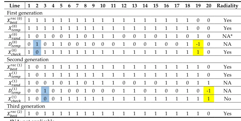
(NR) can be performed by changing the state of sectionalized (closed) and tie (open) switches,
66
considering the need not to lose the radiality of the system. In the literature, NR has been applied in
67
different works to minimize network losses, improve the voltage profile, balance loads between two
68
or more feeders, and reduce the need for network reinforcement, while considering the influence and
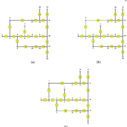
69
increase of penetration of the DG units [6]. Also, the NR problem can be solved while taking into
70
account the optimal placement of shunt capacitors [11], harmonic filters [12] and power electronic
71
devices [13] to control the flow of either reactive and active powers or both between the feeders they
72
are connected to, because the extra power conditioners may be beneficial in some cases to enhance
73
the operational flexibility of the existing configurations, leading to more cumulative benefits of
74
reduced losses.
75
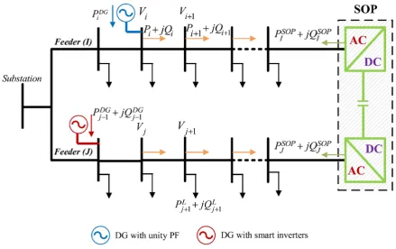
In this regard, soft open points (SOPs) are power electronic devices that can be placed instead of
76
normally open/closed points to provide a fast response, frequent actions and enhanced control
77
scheme for power flow between adjacent feeders they are connected to. In the near past, the optimal
78
operation of SOPs was investigated in balanced and unbalanced active distribution networks [14],
79
[15]. Several design strategies are manipulated for their optimal operation, such as the minimization
80
of energy loss [15] or annual expense [16] in a system, loads balancing [17], voltage profile
81
enhancement [18], and increasing the renewables hosting capacity [19] in distribution systems.
82
Various single-objective and multi-objective optimization techniques were used to solve these
83
optimization problems. Table 1 presents an overview of research works that have addressed SOPs
84
design and operation [15]–[34].
85
Some researchers such as Xiao et al. [34] did not consider the active power loss of the SOP
86
although there is active power loss in the SOP itself. However, they assumed that the active power
87
loss of the SOP is relatively small when compared to the entire distribution system losses. On the
88
other hand, the impact of the internal active losses of SOPs was presented in many research works,
89
but the influence of SOPs’ power loss on the system performance, its share in the total active power
90
loss, and the effect of increasing the number of SOPs connected to the system are not investigated in
91
these works. Also, throughout the literature, one can see that most of the studies concerned with NR
92
and SOPs assume a fixed number and location of the SOP, which might not result in optimal
93
operational performance, in addition to permitting reverse power flow in the systems considered in
94
these studies. Moreover, optimizing the NR, DGs allocation and SOPs placement strategies separately
95
has some drawbacks, such as the lack of collaboration between strategies, which may lead to
sub-96
optimal overall performance and an inability to model the correlation between the benefits of each
97
strategy. To redress these gaps, in this study, we are motivated to allocate SOPs and DGs
98
simultaneously with and without NR and investigate the contribution of SOP losses to the total active
99
losses, as well as the effect of increasing the number of SOPs connected to the studied systems under
100
different loading conditions to determine the real benefits gained from each strategy. In addition, an
101
analytical NR approach is proposed to obtain radial configurations in an efficient manner without
102
the possibility of getting trapped in local minima. Further, multi-scenario studies, which aim to
103
improve the investigation of the overall performance of the strategies, are conducted on an IEEE
33-104
node balanced benchmark distribution system and an 83-node balanced distribution system from a
105
Table 1. Overview of research works addressing SOPs design and operation
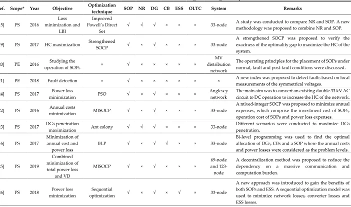
107
Ref. Scope* Year Objective Optimization
technique SOP NR DG CB ESS OLTC System Remarks
[15] PS 2016
Loss minimization and
LBI
Improved Powell’s Direct
Set
√ √ √ × × × 33-node A study was conducted to compare NR and SOP. A new methodology was proposed to combine NR and SOP.
[19] PS 2017 HC maximization Strengthened
SOCP √ × √ × × × 33-node
A strengthened SOCP was proposed to verify the exactness of the optimality gap to maximize the HC of the system.
[20] PE 2016 Studying the
operation of SOPs × √ × × × × ×
MV distribution
network
The operating principles for the placement of SOPs under normal, fault and post-fault conditions were discussed.
[21] PE 2018 Fault detection × √ × × × × × × A new index was proposed to detect faults based on local measurements of the symmetrical voltages.
[24] PS 2017 minimization Power loss PSO √ × √ × × × Anglesey network The main aim was to convert an existing double 33 kV AC circuit to DC operation to increase the HC of the network.
[22] PS 2016 Annual costs
minimization MISOCP √ × √ × × × 33-node
A mixed-integer SOCP was proposed to minimize annual expenses, which comprise the investment cost of SOPs, operation cost of SOPs and power loss expenses.
[23] PS 2017 DGs penetration maximization Ant colony √ √ √ × × × 33-node Different scenarios were conducted to maximize DGs penetration.
[16] PS 2017
Minimization of annual cost and
power loss
BLP √ × √ √ × × 33-node
Bi-level programming was used to find the optimal allocation of DGs, CBs and a SOP where the annual costs and power losses were considered as the problem levels.
[25] PS 2019
Combined minimization of total power loss
and VD
MISOCP √ × √ × × ×
69-node and 123-node
A decentralization method was proposed to reduce the dependency on a massive communication and computation burden.
[26] PS 2018 Power loss minimization
Sequential
optimization √ × √ × √ × 33-node
Ref. Scope* Year Objective Optimization
technique SOP NR DG CB ESS OLTC System Remarks
[27] PS 2016 HC maximization × √ × √ × × × Generic
system
HC maximization gained from insertion of a SOP between two distinct 33 kV networks were presented. [28] PS 2016 Power loss
minimization MISOCP √ √ √ × × × 33-node
A new methodology to allocate a SOP along with NR simultaneously considering the cost of switching actions and SOP losses was presented.
[29] PS 2017 Minimization of
ESS costs MISOCP √ √ √ × √ √ 33-node
Optimally sited and sized ESSs in an ADN that includes SOP and DGs smart inverters were presented.
[30] PS 2017 loss minimization LBI and power SOCP √ × √ × × × 33-node Installation of a multi-terminal SOP using an enhanced SOCP-based method was proposed.
[31] PS 2018 Restored loads maximization
Primal-dual
interior-point √ × √ × √ ×
33-node and 123-node
SOP islanding partitioning of ADNs with DGs, loads and ESSs time series characteristics was presented.
[32] PS 2017
Operation cost and VD minimization
MISOCP √ × √ √ √ √
33-node and 123-node
Optimal coordination between OLTC, CBs and SOP using a time-series model was presented.
[17] PE 2016
VD, LBI and energy loss minimization
Interior-point √ × √ × × ×
MV distribution
network
A Jacobian matrix-based sensitivity method was proposed to operate a SOP under various conditions.
[18] PS 2017
Power loss, LBI and VD minimization
MOPSO and
Taxicab √ √ √ × × × 69-node
Optimal allocation of SOP with NR at various DGs penetrations was presented.
[33] PS 2017 Annual expenses
minimization MISOCP √ √ √ × × ×
33-node and
83-node
A new concept was presented to install SOPs in normally closed lines as well as normally open lines.
[34] PS 2018 Voltage imbalance
Improved differential
evolution algorithm
√ × √ × × ×
Hybrid distribution
system
Optimal allocation of SOPs to improve 3-phase imbalance with DGs and loads uncertainties were proposed using an improved differential evolution algorithm.
The multi-scenario studies investigated in this work are: 1) NR as a stand-alone strategy, 2) DGs
109
allocation as a stand-alone strategy, 3) simultaneous NR and DGs allocation, 4) SOPs allocation
110
without NR, 5) SOPs allocation after NR is performed, 6) simultaneous SOPs allocation and NR, 7)
111
simultaneous SOPs and DGs allocation without NR, 8) simultaneous SOPs and DGs allocation after
112
NR is performed, and 9) simultaneous NR and SOPs and DGs allocation.
113
A recent meta-heuristic optimization algorithm called the discrete-continuous hyper-spherical
114
search (DC-HSS) algorithm is used to solve the mixed-integer nonlinear problem (MINLP) of SOPs
115
and DGs allocation along with NR to minimize power loss in the distribution systems. The DC-HSS
116
has the advantages of fast convergence to the optimal/near-optimal solutions [35], [36].
117
The contribution of this work is twofold. First, we propose a new NR methodology to obtain the
118
possible radial configurations from random configurations to minimize power loss in two
119
distribution systems, taking into account different strategies for DGs, SOPs, and NR while
120
considering multi-scenarios to improve the investigation of the overall performance of the
121
strategies, and in turn their priorities. Second, the contribution of SOP losses to the total active losses
122
as well as the effect of increasing the number of SOPs connected to the system are investigated under
123
different loading conditions to determine the real benefits gained from SOPs and DGs allocation with
124
network reconfiguration to provide the best operation of distribution networks with minimum losses
125
and enhanced power quality performance. It was clear from the results obtained that placing SOPs
126
and DGs into a distribution system creates a hybrid configuration that merges the benefits offered by
127
radial and meshed distribution systems and mitigates drawbacks related to losses, PQ, and voltage
128
violations, while offering far more efficient and optimal network operation.
129
The rest of the paper is organized as follows: Section II presents the problem statement, proposed
130
NR methodology, modeling of SOPs and DGs, and PQ indices that evaluate the system performance.
131
Further, Section III presents the problem formulation and the search algorithm used to solve the
132
mixed-integer nonlinear problem. Section IV presents the results and discusses them, and Section V
133
presents the conclusions and limitations of our study as well as a preview of future works.
134
2. Problem Statement
135
The NR, SOPs and DGs modeling, and PQ performance indices, namely the load balancing index
136
(LBI), and aggregate voltage deviation index (AVDI), are presented and discussed. Hence, the
137
formulation of the load flow calculations, the objective function to minimize the network active
138
power loss, the constraint conditions of voltage, current, SOP capacity, active and reactive powers,
139
and the DC-HSS algorithm proposed to solve the formulated MINLP problem are presented.
140
2.1. Proposed Network Reconfiguration
141
Distribution systems have sectionalizing switches (normally closed switches) that connect line
142
sections and tie switches (normally open switches) that connect two primary feeders, two substation
143
buses, or loop-type laterals. Each line is assumed a sectionalized line with a normally closed
144
sectionalized switch in the line. Also, each normally open tie switch is assumed to be in each tie line.
145
Thus, NR is the change that occurs in the status of tie and sectionalized switches to reconnect
146
distribution feeders to form a new radial structure for a certain operation goal without violating the
147
condition of having a radial structure. In this study, the procedure of NR to generate possible radial
148
configurations in a fast and efficient manner is implemented analytically and is clarified as follows:
149
Step 1: A binary vector 𝑋𝑋𝑝𝑝𝑝𝑝𝑛𝑛𝑟𝑟(0) = [1 0 0 1 1 … 1]1×𝑁𝑁𝑏𝑏𝑏𝑏 is initialized with random binary values, in
150
which its length is equal to the number of lines (𝑁𝑁𝑏𝑏𝑝𝑝) with its sectionalized and tie switches. The
151
sectionalized switches are denoted "1" and the tie switches are denoted "0".
152
Step 2: The best reconfiguration vector of the system (𝑋𝑋𝑏𝑏𝑝𝑝𝑙𝑙𝑝𝑝𝑝𝑝𝑝𝑝𝑝𝑝), which represents the best vector that
153
meets the radiality requirements (described in Step 6) and achieves the desired goal, is initialized
154
with the base configuration of the system.
155
Step 3: A temporary vector 𝑋𝑋𝑝𝑝𝑝𝑝𝑚𝑚𝑝𝑝(0) that is equal to 𝑋𝑋𝑏𝑏𝑝𝑝𝑙𝑙𝑝𝑝𝑝𝑝𝑝𝑝𝑝𝑝 is created. At that point, each element in
156
𝐴𝐴𝑝𝑝𝑝𝑝𝑚𝑚𝑝𝑝(0) =𝑋𝑋𝑝𝑝𝑝𝑝𝑚𝑚𝑝𝑝(0) − 𝑋𝑋𝑝𝑝𝑝𝑝𝑛𝑛𝑟𝑟(0) . Further, ∀𝑏𝑏 ∈ 𝑁𝑁𝑏𝑏𝑝𝑝, if 𝐴𝐴𝑝𝑝𝑝𝑝𝑚𝑚𝑝𝑝(0) (𝑏𝑏) = 1, it means that this bth line is changed to
158
a tie line in the random vector; also if 𝐴𝐴𝑝𝑝𝑝𝑝𝑚𝑚𝑝𝑝(0) (𝑏𝑏) =−1 , it means that the bth line is changed to a
159
sectionalized line in the random vector. Otherwise, if 𝐴𝐴𝑝𝑝𝑝𝑝𝑚𝑚𝑝𝑝(0) (𝑏𝑏) = 0, this indicates that no change has
160
occurred.
161
Step 4: Starting from the first element in 𝐴𝐴𝑝𝑝𝑝𝑝𝑚𝑚𝑝𝑝(0) , if 𝐴𝐴𝑝𝑝𝑝𝑝𝑚𝑚𝑝𝑝(0) (𝑏𝑏) = 1 and 𝐴𝐴𝑝𝑝𝑝𝑝𝑚𝑚𝑝𝑝(0) (𝑗𝑗) =−1 , where 𝑗𝑗
162
denotes a random line selected from the remaining lines in the system with the condition that 𝑏𝑏 ≠ 𝑗𝑗,
163
a vector 𝑋𝑋𝑝𝑝ℎ𝑝𝑝𝑝𝑝𝑒𝑒(0) is generated so that 𝑋𝑋𝑝𝑝ℎ𝑝𝑝𝑝𝑝𝑒𝑒(0) is equal to 𝑋𝑋𝑝𝑝𝑝𝑝𝑚𝑚𝑝𝑝(0) subjected to 𝑋𝑋𝑝𝑝ℎ𝑝𝑝𝑝𝑝𝑒𝑒(0) (𝑏𝑏) = 0 and
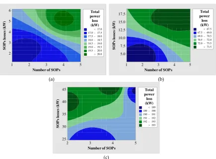
164
𝑋𝑋𝑝𝑝ℎ𝑝𝑝𝑝𝑝𝑒𝑒(0) (𝑗𝑗) = 1. The vector 𝑋𝑋𝑝𝑝ℎ𝑝𝑝𝑝𝑝𝑒𝑒(0) is then checked for radiality described in Step 6. If it is found to be
165
radial, then 𝑏𝑏 is updated so that 𝑏𝑏=𝑏𝑏+ 1, and the vector 𝑋𝑋𝑝𝑝𝑝𝑝𝑚𝑚𝑝𝑝(1) is generated equal to 𝑋𝑋𝑏𝑏𝑝𝑝𝑙𝑙𝑝𝑝𝑝𝑝𝑝𝑝𝑝𝑝 (1). It
166
should be mentioned that a set of 𝑋𝑋𝑝𝑝ℎ𝑝𝑝𝑝𝑝𝑒𝑒(0) vectors may be generated as soon as 𝑏𝑏 is smaller than or
167
equal to 𝑁𝑁𝑏𝑏𝑝𝑝, and the vectors found to be radial in this set are evaluated based on their fitness value
168
to give the best 𝑋𝑋𝑏𝑏𝑝𝑝𝑙𝑙𝑝𝑝𝑝𝑝𝑝𝑝𝑝𝑝.
169
Step 5: The steps will terminate when we achieve a very small distance among serial solutions by
170
evaluation of the objective function.
171
Step 6: The procedure of radiality check is done as follows:
172
• Build an incidence matrix 𝑀𝑀 where its rows and columns represent the lines and nodes of the
173
distribution network, respectively. The nodes of each line are denoted “1” in 𝑀𝑀, and the rest of
174
the elements in the row are denoted “0”.
175
• Elements in the rows of each tie line are set to “0”. Then, we create a vector 𝐷𝐷, in which its length
176
is equal to the number of nodes, and each element 𝑒𝑒 in 𝐷𝐷 is equal to the sum of its corresponding
177
𝑒𝑒𝑝𝑝ℎ column in 𝑀𝑀. If an element in 𝐷𝐷 is equal to “1”, it means that this element represents an end
178
node. Further, the row that corresponds to this end node in 𝑀𝑀 is set to “0”.
179
• Recalculate 𝐷𝐷 and repeat the former process as soon as an element in 𝐷𝐷 is equal to 1. At that
180
point, calculate the sum of all the elements in 𝑀𝑀. If the sum is equal to zero, this means that the
181
configuration is radial, otherwise, it is not radial.
182
An illustrative example for a 19-node system is given in Table 2 to clarify the proposed
183
reconfiguration procedure, in which the lines changed to ties are shaded blue, and the lines changed
184
to sectionalized are shaded yellow. Fig. 1(a) shows the initial configuration of the 19-node system.
185
Figs. 1(b) and 1(c) show two possible attempts to obtain a new configuration of the system in the first
186
two generations of the reconfiguration procedure. From that, it can be noted that the proposed
187
algorithm can produce a series of radial configurations and modify the obtained non-radial
188
configurations to be radial.
189
Table 2.Proposed NR Procedure
190
Line 1 2 3 4 5 6 7 8 9 10 11 12 13 14 15 16 17 18 19 20 Radiality
First generation
𝑋𝑋𝑏𝑏𝑝𝑝𝑙𝑙𝑝𝑝𝑝𝑝𝑝𝑝𝑝𝑝 (0) 1 1 1 1 1 1 1 1 1 1 1 1 1 1 1 1 1 1 0 0 Yes 𝑋𝑋𝑝𝑝𝑝𝑝𝑚𝑚𝑝𝑝(0) 1 1 1 1 1 1 1 1 1 1 1 1 1 1 1 1 1 1 0 0 Yes 𝑋𝑋𝑝𝑝𝑝𝑝𝑛𝑛𝑟𝑟(0) 1 0 1 0 0 1 1 0 1 1 1 0 0 1 0 1 1 0 1 0 NA* 𝐴𝐴𝑝𝑝𝑝𝑝𝑚𝑚𝑝𝑝(0) 0 1 0 1 1 0 0 1 0 0 0 1 0 0 1 0 0 1 -1 0 NA 𝑋𝑋𝑝𝑝ℎ𝑝𝑝𝑝𝑝𝑒𝑒(0) 1 0 1 1 1 1 1 1 1 1 1 1 1 1 1 1 1 1 1 0 Yes
Second generation
𝑋𝑋𝑏𝑏𝑝𝑝𝑙𝑙𝑝𝑝𝑝𝑝𝑝𝑝𝑝𝑝 (1) 1 0 1 1 1 1 1 1 1 1 1 1 1 1 1 1 1 1 1 0 Yes 𝑋𝑋𝑝𝑝𝑝𝑝𝑚𝑚𝑝𝑝(1) 1 0 1 1 1 1 1 1 1 1 1 1 1 1 1 1 1 1 1 0 Yes 𝑋𝑋𝑝𝑝𝑝𝑝𝑛𝑛𝑟𝑟(1) 1 0 0 1 0 1 1 0 1 1 1 0 0 1 0 1 1 0 1 1 NA 𝐴𝐴𝑝𝑝𝑝𝑝𝑚𝑚𝑝𝑝(1) 0 0 1 0 1 0 0 1 0 0 0 1 1 0 1 0 0 1 0 -1 NA 𝑋𝑋𝑝𝑝ℎ𝑝𝑝𝑝𝑝𝑒𝑒(1) 1 0 0 0 1 1 1 1 1 1 1 1 1 1 1 1 1 1 1 1 No Third generation
𝑋𝑋𝑏𝑏𝑝𝑝𝑙𝑙𝑝𝑝𝑝𝑝𝑝𝑝𝑝𝑝 (2) 1 0 1 1 1 1 1 1 1 1 1 1 1 1 1 1 1 1 1 0 Yes *NA: not applicable
(
a)
(
b)
192
(c)
193
Figure 1. Illustrative 19-node distribution system: (a) base configuration, (b) radial configuration generated
194
(𝑿𝑿𝒄𝒄𝒄𝒄𝒄𝒄𝒄𝒄𝒄𝒄(𝟎𝟎) ), and (c) non-radial configuration generated (𝑿𝑿𝒄𝒄𝒄𝒄𝒄𝒄𝒄𝒄𝒄𝒄(𝟏𝟏) ).
195
196
2.2. SOP Modeling
197
SOPs were first presented in 2011 [39] to provide resilience between distribution feeders. They
198
can be integrated in distribution networks using three topologies, comprising a back-to-back (B2B)
199
voltage source converter (VSC), static series synchronous compensator and unified power flow
200
controller [40]. In this work, we used a B2B-VSC as the integration topology for SOPs connected to
201
the studied systems because of its flexibility and dynamic capability to enhance the power quality.
202
Fig. 2 shows an illustration of SOPs integration into a distribution system. To model a SOP, the main
203
equations to model the flow of power in the network under study are expressed as follows:
204
𝑃𝑃𝑝𝑝+1=𝑃𝑃𝑝𝑝− 𝑃𝑃𝑝𝑝+1𝐿𝐿 − 𝑟𝑟𝑝𝑝,𝑝𝑝+1∙𝑃𝑃𝑝𝑝 2+𝑄𝑄
𝑝𝑝2
|𝐴𝐴𝑝𝑝|2 (1)
205
𝑄𝑄𝑝𝑝+1=𝑄𝑄𝑝𝑝− 𝑄𝑄𝑝𝑝+1𝐿𝐿 − 𝑥𝑥𝑝𝑝,𝑝𝑝+1∙𝑃𝑃𝑝𝑝 2+𝑄𝑄
𝑝𝑝 2
|𝐴𝐴𝑝𝑝|2 (2)
206
|𝐴𝐴𝑝𝑝+1|2= |𝐴𝐴𝑝𝑝|2−2�𝑟𝑟𝑝𝑝,𝑝𝑝+1∙ 𝑃𝑃𝑝𝑝+𝑥𝑥𝑝𝑝,𝑝𝑝+1∙ 𝑄𝑄𝑝𝑝�+�𝑟𝑟𝑝𝑝2,𝑝𝑝+1+𝑥𝑥𝑝𝑝2,𝑝𝑝+1�𝑃𝑃𝑝𝑝 2+𝑄𝑄
𝑝𝑝2
|𝐴𝐴𝑝𝑝|2 (3)
207
209
Figure 2. Illustration of SOPs integration into a distribution system
210
active and reactive powers of the connected loads onto node 𝑖𝑖+ 1, |𝐴𝐴𝑝𝑝| is the magnitude of the 𝑖𝑖𝑝𝑝ℎ
211
node voltage and 𝑟𝑟𝑝𝑝,𝑝𝑝+1 and 𝑥𝑥𝑝𝑝,𝑝𝑝+1 are the feeder resistance and reactance between nodes 𝑖𝑖 and 𝑖𝑖+
212
1.
213
Then, the SOP is integrated using its active and reactive powers injected at its terminals as
214
presented in Fig. 2, in which the summation of the injected powers at the SOP terminals and the
215
internal power loss of its converters must equal zero, as expressed in (4). Thus:
216
𝑃𝑃𝐼𝐼𝑆𝑆𝑆𝑆𝑆𝑆+𝑃𝑃𝐽𝐽𝑆𝑆𝑆𝑆𝑆𝑆+𝑃𝑃𝐼𝐼𝑆𝑆𝑆𝑆𝑆𝑆−𝑙𝑙𝑙𝑙𝑙𝑙𝑙𝑙+𝑃𝑃𝐽𝐽𝑆𝑆𝑆𝑆𝑆𝑆−𝑙𝑙𝑙𝑙𝑙𝑙𝑙𝑙= 0 (4)
217
The reactive power limits are given in (5) and the SOP capacity limit is shown in (6). Thus:
218
𝑄𝑄𝐼𝐼𝑆𝑆𝑆𝑆𝑆𝑆−𝑚𝑚𝑝𝑝𝑛𝑛≤ 𝑄𝑄𝐼𝐼𝑆𝑆𝑆𝑆𝑆𝑆≤ 𝑄𝑄𝐼𝐼𝑆𝑆𝑆𝑆𝑆𝑆−𝑚𝑚𝑝𝑝𝑚𝑚,∀𝐴𝐴,𝐽𝐽 ∈ 𝑁𝑁𝑜𝑜 (5)
219
�(𝑃𝑃𝐼𝐼𝑆𝑆𝑆𝑆𝑆𝑆)2+ (𝑄𝑄𝐼𝐼𝑆𝑆𝑆𝑆𝑆𝑆)2≤ 𝐷𝐷𝐼𝐼𝑆𝑆𝑆𝑆𝑆𝑆,∀𝐴𝐴 ∈ 𝑁𝑁𝑜𝑜 (6)
220
where 𝑁𝑁𝑜𝑜 is the number of feeders, 𝑃𝑃𝐼𝐼𝑆𝑆𝑆𝑆𝑆𝑆 is the SOP’s active power injected to the 𝐴𝐴𝑝𝑝ℎ feeder, 𝑃𝑃𝐽𝐽𝑆𝑆𝑆𝑆𝑆𝑆
221
is the SOP’s active power to the 𝐽𝐽𝑝𝑝ℎ feeder, 𝑃𝑃
𝐼𝐼𝑆𝑆𝑆𝑆𝑆𝑆−𝑙𝑙𝑙𝑙𝑙𝑙𝑙𝑙 is the active power loss of the converter
222
connected to the 𝐴𝐴𝑝𝑝ℎ feeder, 𝑃𝑃
𝐽𝐽𝑆𝑆𝑆𝑆𝑆𝑆−𝑙𝑙𝑙𝑙𝑙𝑙𝑙𝑙 is the internal power loss of the converter connected to the
223
𝐽𝐽𝑝𝑝ℎ feeder, 𝑄𝑄
𝐼𝐼𝑆𝑆𝑆𝑆𝑆𝑆 is the SOP’s reactive power injected to the 𝐴𝐴𝑝𝑝ℎ feeder,𝑄𝑄𝐽𝐽𝑆𝑆𝑆𝑆𝑆𝑆 is the SOP’s reactive
224
power injected to the 𝐽𝐽𝑝𝑝ℎ feeder, 𝑄𝑄
𝐼𝐼𝑆𝑆𝑆𝑆𝑆𝑆−𝑚𝑚𝑝𝑝𝑛𝑛 and 𝑄𝑄𝐼𝐼𝑆𝑆𝑆𝑆𝑆𝑆−𝑚𝑚𝑝𝑝𝑚𝑚 are the minimum and maximum limits
225
of the SOP’s reactive power injected to the 𝐴𝐴𝑝𝑝ℎ feeder, and 𝐷𝐷
𝐼𝐼𝑆𝑆𝑆𝑆𝑆𝑆 is the maximum capacity limit of
226
the planned SOP. Further, the active loss of each converter (𝑃𝑃𝐼𝐼𝑆𝑆𝑆𝑆𝑆𝑆−𝑙𝑙𝑙𝑙𝑙𝑙𝑙𝑙 and 𝑃𝑃𝐽𝐽𝑆𝑆𝑆𝑆𝑆𝑆−𝑙𝑙𝑙𝑙𝑙𝑙𝑙𝑙) and the total
227
SOPs active power loss (𝑃𝑃𝑆𝑆𝑆𝑆𝑆𝑆−𝑙𝑙𝑙𝑙𝑙𝑙𝑙𝑙) are formulated in (7) and (8) as follows [32]:
228
𝑃𝑃𝑆𝑆𝑆𝑆𝑆𝑆−𝑙𝑙𝑙𝑙𝑙𝑙𝑙𝑙 = � 𝑃𝑃
𝐼𝐼𝑆𝑆𝑆𝑆𝑆𝑆−𝑙𝑙𝑙𝑙𝑙𝑙𝑙𝑙 𝑁𝑁𝑓𝑓
𝐼𝐼=1
(7)
229
𝑃𝑃𝐼𝐼𝑆𝑆𝑆𝑆𝑆𝑆−𝑙𝑙𝑙𝑙𝑙𝑙𝑙𝑙=𝐴𝐴𝑙𝑙𝑙𝑙𝑙𝑙𝑙𝑙𝑆𝑆𝑆𝑆𝑆𝑆�(𝑃𝑃𝐼𝐼𝑆𝑆𝑆𝑆𝑆𝑆)2+ (𝑄𝑄𝐼𝐼𝑆𝑆𝑆𝑆𝑆𝑆)2,∀𝐴𝐴 ∈ 𝑁𝑁𝑜𝑜 (8)
230
where 𝐴𝐴𝑙𝑙𝑙𝑙𝑙𝑙𝑙𝑙𝑆𝑆𝑆𝑆𝑆𝑆 is the loss coefficient of VSCs, which represents leakage in the transferred power to the
231
total power transferred between feeders [32]-[34].
232
Mathematically, to represent the SOP variables, first, we can consider a lossless SOP, i.e.
233
𝑃𝑃𝐼𝐼𝑆𝑆𝑆𝑆𝑆𝑆−𝑙𝑙𝑙𝑙𝑙𝑙𝑙𝑙= 0,∀𝐴𝐴 ∈ 𝑁𝑁𝑜𝑜; hence, a SOP can be represented by its injected active and reactive powers
234
�𝑃𝑃𝐼𝐼𝑆𝑆𝑆𝑆𝑆𝑆,𝑄𝑄𝐼𝐼𝑆𝑆𝑆𝑆𝑆𝑆,𝑄𝑄𝐽𝐽𝑆𝑆𝑆𝑆𝑆𝑆�, where 𝑃𝑃𝐽𝐽𝑆𝑆𝑆𝑆𝑆𝑆=−𝑃𝑃𝐼𝐼𝑆𝑆𝑆𝑆𝑆𝑆. Therefore, multiple SOPs can be modeled by the vector
235
�𝑃𝑃𝐼𝐼𝑆𝑆𝑆𝑆𝑆𝑆(1),𝑄𝑄𝐼𝐼𝑆𝑆𝑆𝑆𝑆𝑆(1),𝑄𝑄𝐽𝐽𝑆𝑆𝑆𝑆𝑆𝑆(1), …𝑃𝑃𝑀𝑀𝑆𝑆𝑆𝑆𝑆𝑆(𝑛𝑛),𝑄𝑄𝑀𝑀𝑆𝑆𝑆𝑆𝑆𝑆(𝑛𝑛),𝑄𝑄𝐾𝐾𝑆𝑆𝑆𝑆𝑆𝑆(𝑛𝑛)� such that the first three variables in the
236
vector represent the first SOP connected between the Ith and Jth feeders, while the last three variables
237
Second, we can consider the SOP with its losses taken into account, i.e. 𝑃𝑃𝐼𝐼𝑆𝑆𝑆𝑆𝑆𝑆−𝑙𝑙𝑙𝑙𝑙𝑙𝑙𝑙 ≠0,∀𝐴𝐴 ∈ 𝑁𝑁𝑜𝑜;
239
hence, starting from (4), we can get 𝑃𝑃𝐼𝐼𝑆𝑆𝑆𝑆𝑆𝑆−𝑙𝑙𝑙𝑙𝑙𝑙𝑙𝑙 as follows:
240
𝑃𝑃𝐽𝐽𝑆𝑆𝑆𝑆𝑆𝑆=−𝑃𝑃𝐼𝐼𝑆𝑆𝑆𝑆𝑆𝑆− 𝑃𝑃𝐼𝐼𝑆𝑆𝑆𝑆𝑆𝑆−𝑙𝑙𝑙𝑙𝑙𝑙𝑙𝑙− 𝑃𝑃𝐽𝐽𝑆𝑆𝑆𝑆𝑆𝑆−𝑙𝑙𝑙𝑙𝑙𝑙𝑙𝑙 (9)
241
Substituting (8) into (9), then
242
𝑃𝑃𝐽𝐽𝑆𝑆𝑆𝑆𝑆𝑆=−𝑃𝑃𝐼𝐼𝑆𝑆𝑆𝑆𝑆𝑆− 𝐴𝐴𝑆𝑆𝑆𝑆𝑆𝑆𝑙𝑙𝑙𝑙𝑙𝑙𝑙𝑙�(𝑃𝑃𝐼𝐼𝑆𝑆𝑆𝑆𝑆𝑆)2+ (𝑄𝑄𝐼𝐼𝑆𝑆𝑆𝑆𝑆𝑆)2− 𝐴𝐴𝑙𝑙𝑙𝑙𝑙𝑙𝑙𝑙𝑆𝑆𝑆𝑆𝑆𝑆��𝑃𝑃𝐽𝐽𝑆𝑆𝑆𝑆𝑆𝑆�2+�𝑄𝑄𝐽𝐽𝑆𝑆𝑆𝑆𝑆𝑆�2 (10)
243
Accordingly, if we set 𝑃𝑃𝐼𝐼𝑆𝑆𝑆𝑆𝑆𝑆,𝑄𝑄𝐼𝐼𝑆𝑆𝑆𝑆𝑆𝑆and 𝑄𝑄𝐽𝐽𝑆𝑆𝑆𝑆𝑆𝑆 as the SOP’s decision variables, (10) will be a
244
nonlinear equation with one unknown �𝑃𝑃𝐽𝐽𝑆𝑆𝑆𝑆𝑆𝑆�. So, it can be independently solved using numerical
245
analysis methods such as Newton’s method to find the value of the root (𝑃𝑃𝐽𝐽𝑆𝑆𝑆𝑆𝑆𝑆) of (10). Therefore,
246
assuming that 𝐴𝐴𝑙𝑙𝑙𝑙𝑙𝑙𝑙𝑙𝑆𝑆𝑆𝑆𝑆𝑆 is known; a SOP can be represented by its injected active and reactive powers
247
�𝑃𝑃𝐼𝐼𝑆𝑆𝑆𝑆𝑆𝑆,𝑄𝑄𝐼𝐼𝑆𝑆𝑆𝑆𝑆𝑆,𝑄𝑄𝐽𝐽𝑆𝑆𝑆𝑆𝑆𝑆� as the lossless SOP case.
248
2.3. DG Modeling
249
In this study, we used two types of DGs. The first type includes generators with unity power
250
factor and the second is DGs with smart inverters with a reactive power compensation capability
251
within specified limits of the reactive power.
252
The DGs with unity PF are limited by the maximum capacity limit (𝐷𝐷𝐷𝐷𝐷𝐷) of the installed DGs as
253
follows:
254
0≤ 𝑃𝑃𝑝𝑝𝐷𝐷𝐷𝐷≤ 𝐷𝐷𝐷𝐷𝐷𝐷 (11)
255
where 𝑃𝑃𝑝𝑝𝐷𝐷𝐷𝐷is the active DG power injected at the 𝑖𝑖𝑝𝑝ℎ node.
256
In the second type of DG, the reactive power varies based on specified PF limits, so that −𝛽𝛽𝑚𝑚𝑝𝑝𝑛𝑛 and
257
𝛽𝛽𝑚𝑚𝑝𝑝𝑛𝑛are the minimum leading and lagging PF values.
258
�(𝑃𝑃𝑝𝑝𝐷𝐷𝐷𝐷)2+ (𝑄𝑄𝑝𝑝𝐷𝐷𝐷𝐷)2≤ 𝐷𝐷𝐷𝐷𝐷𝐷 (12)
259
−tan(𝑐𝑐𝑐𝑐𝑐𝑐−1𝛽𝛽
𝑚𝑚𝑝𝑝𝑛𝑛)∙ 𝑃𝑃𝑝𝑝𝐷𝐷𝐷𝐷 ≤ 𝑄𝑄𝑝𝑝𝐷𝐷𝐷𝐷≤ 𝑡𝑡𝑀𝑀𝑛𝑛(𝑐𝑐𝑐𝑐𝑐𝑐−1𝛽𝛽𝑚𝑚𝑝𝑝𝑛𝑛)∙ 𝑃𝑃𝑝𝑝𝐷𝐷𝐷𝐷 (13)
260
where 𝑄𝑄𝑝𝑝𝐷𝐷𝐷𝐷 is the reactive DG power injected at the 𝑖𝑖𝑝𝑝ℎ node.
261
2.4. PQ Indices
262
In power distribution systems, apart from the functions that describe the objective and
263
constraints that assess the operational performance, there are other indices that evaluate the impacts
264
of the proposed solution on the PQ performance of the studied systems, such as the load balancing
265
index (𝐿𝐿𝐿𝐿𝐴𝐴), and aggregate voltage deviation index (𝐴𝐴𝐴𝐴𝐴𝐴𝐴𝐴). The mathematical expressions for these
266
quantities are given as follows:
267
2.4.1. Load Balancing Index (LBI)
268
Changing the state of the switches of a distribution system will change its topography. In turn,
269
the loads between the feeders can be distributed to balance the system and avoid the overloading of
270
feeders. In this work, the balancing index (𝐿𝐿𝐿𝐿𝐴𝐴) is used to reflect the loading level of each line in the
271
distribution network [15]. The 𝐿𝐿𝐿𝐿𝐴𝐴 of the 𝑏𝑏𝑝𝑝ℎ line is formulated as follows:
272
𝐿𝐿𝐿𝐿𝐴𝐴𝑏𝑏 =�𝐴𝐴 𝐴𝐴𝑏𝑏 𝑏𝑏𝑝𝑝𝑝𝑝𝑝𝑝𝑝𝑝𝑟𝑟�
2
,∀𝑏𝑏 ∈ 𝑁𝑁𝑏𝑏𝑝𝑝 (14)
273
where 𝐴𝐴𝑏𝑏 is the current flowing in line 𝑏𝑏 and is limited by its rated value 𝐴𝐴𝑏𝑏𝑝𝑝𝑝𝑝𝑝𝑝𝑝𝑝𝑟𝑟 and 𝑁𝑁𝑏𝑏𝑝𝑝 is the
274
number of lines. Hence, the total load balancing index 𝐿𝐿𝐿𝐿𝐴𝐴𝑝𝑝𝑙𝑙𝑝𝑝 is expressed as the sum of the balancing
275
indices of the lines, thus:
276
𝐿𝐿𝐿𝐿𝐴𝐴𝑝𝑝𝑙𝑙𝑝𝑝 =� 𝐿𝐿𝐿𝐿𝐴𝐴𝑏𝑏 𝑁𝑁𝑏𝑏𝑏𝑏
𝑏𝑏=1
(15)
277
𝐿𝐿𝐿𝐿𝐴𝐴 of a certain line decreases if the total load connected to this line decreases, and hence, the
278
line current decreases. However, line currents may increase in other lines, increasing their 𝐿𝐿𝐿𝐿𝐴𝐴s. For
279
that, the 𝐿𝐿𝐿𝐿𝐴𝐴𝑝𝑝𝑙𝑙𝑝𝑝 is calculated for all branches to help determine the overall load balancing of all lines
280
2.4.2. Aggregate voltage deviation index (AVDI)
282
Voltage deviation is a measure of the voltage quality in the system. It is formulated as the
283
summation of voltage deviations at all nodes in the system from a reference value of 1 per unit, and
284
it is given as:
285
𝐴𝐴𝐴𝐴𝐴𝐴𝐴𝐴=�|𝐴𝐴𝑝𝑝−1| 𝑁𝑁𝑛𝑛
𝑝𝑝=1
(16)
286
where 𝑖𝑖 and 𝑁𝑁𝑛𝑛 are the node number and total number of nodes, respectively. A system with lower
287
𝐴𝐴𝐴𝐴𝐴𝐴𝐴𝐴 indicates a secure system with reduced voltage violations.
288
3. Problem Statement
289
3.1. Objective Function
290
The main aim of this work is to minimize the total power loss (𝑃𝑃𝑙𝑙𝑙𝑙𝑙𝑙𝑙𝑙𝑝𝑝𝑙𝑙𝑝𝑝). The objective function 𝑃𝑃𝑙𝑙𝑙𝑙𝑙𝑙𝑙𝑙𝑝𝑝𝑙𝑙𝑝𝑝
291
is divided into two parts, namely the feeder losses due to current flowing in the lines and the SOP’s
292
internal power loss (𝑃𝑃𝑆𝑆𝑆𝑆𝑆𝑆−𝑙𝑙𝑙𝑙𝑙𝑙𝑙𝑙) as expressed in (17).
293
𝑀𝑀𝑖𝑖𝑛𝑛𝑃𝑃𝑙𝑙𝑙𝑙𝑙𝑙𝑙𝑙𝑝𝑝𝑙𝑙𝑝𝑝 =� �𝑃𝑃𝑝𝑝 2+𝑄𝑄
𝑝𝑝2
|𝐴𝐴𝑝𝑝|2 ∙ 𝑟𝑟𝑝𝑝,𝑝𝑝+1� 𝑁𝑁𝑛𝑛
𝑝𝑝=1
+𝜇𝜇 ∙ 𝑃𝑃𝑆𝑆𝑆𝑆𝑆𝑆−𝑙𝑙𝑙𝑙𝑙𝑙𝑙𝑙 (17)
294
where 𝜇𝜇=0 with no SOP losses considered and 𝜇𝜇=1 if SOP losses are considered.
295
3.2. Constraints and Operation Conditions
296
In addition to the radiality requirements described in Section II. A, power flow equality given in
297
(4), SOP reactive power limits given in (5), SOP capacity limit given in (6), SOP active power loss
298
given in (8), DG capacity limit given in (11) for the first type and (12) for the second type, and DG
299
reactive power limits given in (13), the following constraints regarding voltage magnitudes, lines
300
thermal capacities and the total reactive power injected by DGs and/or SOPs into the system are
301
expressed, respectively, as follows:
302
𝐴𝐴𝑚𝑚𝑝𝑝𝑛𝑛≤|𝐴𝐴𝑝𝑝|≤ 𝐴𝐴𝑚𝑚𝑝𝑝𝑚𝑚 (18)
303
|𝐴𝐴b|≤ 𝐴𝐴𝑏𝑏rated,∀𝑏𝑏 ∈ 𝑁𝑁𝑏𝑏𝑝𝑝 (19)
304
� 𝑄𝑄𝑝𝑝𝐷𝐷𝐷𝐷 𝑁𝑁𝐷𝐷𝐷𝐷
𝑝𝑝=1
+ � �𝑄𝑄𝐼𝐼𝑆𝑆𝑆𝑆𝑆𝑆(𝑘𝑘) +𝑄𝑄𝐽𝐽𝑆𝑆𝑆𝑆𝑆𝑆(𝑘𝑘)� 𝑁𝑁𝑆𝑆𝑆𝑆𝑆𝑆
𝑒𝑒=1
≤ � 𝑄𝑄𝑢𝑢𝐿𝐿 𝑁𝑁𝑛𝑛
𝑢𝑢=1
(20)
305
where 𝐴𝐴𝑚𝑚𝑝𝑝𝑛𝑛 and 𝐴𝐴𝑚𝑚𝑝𝑝𝑚𝑚 represent minimum and maximum voltage limits respectively, and 𝑁𝑁𝐷𝐷𝐷𝐷 is the
306
number of connected DGs. It should be noted that the total reactive power injected by DGs and SOPs
307
must not exceed the total demand reactive power, as expressed in (20), to avoid the system’s
over-308
compensation, and to maintain the PF to be within higher lagging values [35], [36]. Also, no reverse
309
power flow is permitted in the system, as expressed in (21). Otherwise, further precautions should
310
be taken by network operators to control excessive reverse power flows and the associated problems
311
resulting from high DG penetration levels.
312
𝑃𝑃𝑝𝑝𝐿𝐿− 𝑀𝑀 ∙ 𝑃𝑃𝑝𝑝𝐷𝐷𝐷𝐷− 𝑏𝑏 ∙ 𝑃𝑃𝐼𝐼𝑆𝑆𝑆𝑆𝑆𝑆− 𝑐𝑐 ∙ 𝑃𝑃𝐽𝐽𝑆𝑆𝑆𝑆𝑆𝑆≥0,∀𝑖𝑖 ∈ 𝑁𝑁𝑛𝑛 (21)
313
where 𝑀𝑀 equals 1 in the case of node 𝑖𝑖 connected to a DG unit, 𝑏𝑏 equals 1 in the case of node 𝑖𝑖
314
connected to a SOP through feeder 𝐴𝐴, and 𝑐𝑐 equals 1 in the case of node 𝑖𝑖 connected to a SOP
315
through feeder 𝐽𝐽; otherwise, 𝑀𝑀=𝑏𝑏=𝑐𝑐= 0.
316
3.3. Search Algorithm
317
The hyper-spherical search (HSS) algorithm was developed by Karami et al. in 2014 [37] to solve
318
nonlinear functions and was further enhanced in 2016 [38] to consider mixed continuous-discrete
319
decision variables to solve MINLP problems. The DC-HSS has the advantages of fast convergence to
320
the optimal/near-optimal solutions and good performance in solving mixed continuous-discrete
321
problems. Therefore, we have used the DC-HSS algorithm to solve our optimization problem.
322
The population is categorized into two types: particles and sphere-centers (SCs). The algorithm
324
searches in the inner space of the hyper-sphere to find a new particle position with a better value of
325
the objective function as follows:
326
Step 1: Initialization: the algorithm starts by assigning the population size �𝑁𝑁𝑝𝑝𝑙𝑙𝑝𝑝�, the distance
327
between the particle and the sphere-center (𝑟𝑟), taking into account random values between [𝑟𝑟𝑚𝑚𝑝𝑝𝑛𝑛,
328
𝑟𝑟max], the number of sphere-centers (𝑁𝑁𝑆𝑆𝑆𝑆), the number of decision variables (𝑁𝑁), the probability of
329
changing the particle’s angle �𝑃𝑃𝑟𝑟𝑝𝑝𝑛𝑛𝑎𝑎𝑙𝑙𝑝𝑝�, and the maximum number of iterations (𝑀𝑀𝑀𝑀𝑥𝑥𝑝𝑝𝑝𝑝𝑝𝑝𝑝𝑝). Then, a
330
vector of decision variables (𝑥𝑥𝑝𝑝) is initialized with random values between [𝑋𝑋𝑝𝑝𝑚𝑚𝑝𝑝𝑛𝑛, 𝑋𝑋𝑝𝑝max] by a
331
uniform probability function. A set equal to 𝑁𝑁𝑝𝑝𝑙𝑙𝑝𝑝 containing the objective function values is formed
332
for each vector, in which each vector of the decision variables [𝑥𝑥1,𝑥𝑥2, … ,𝑥𝑥𝑁𝑁] is named as a particle.
333
Further, the particles are sorted according to their objective function values, and then the best 𝑁𝑁𝑆𝑆𝑆𝑆
334
particles with the lowest objective function are selected as the initial sphere-centers. The rest of the
335
particles (𝑁𝑁𝑝𝑝𝑙𝑙𝑝𝑝− 𝑁𝑁𝑆𝑆𝑆𝑆) are then distributed among the sphere-centers. Finally, a distribution of the
336
(𝑁𝑁𝑝𝑝𝑙𝑙𝑝𝑝− 𝑁𝑁𝑆𝑆𝑆𝑆) particles among the SCs is performed by the objective function difference (𝐷𝐷𝐷𝐷𝐴𝐴) for each
337
SC, where the 𝐷𝐷𝐷𝐷𝐴𝐴 is equal to the objective function of SC (𝑓𝑓𝑆𝑆𝑆𝑆) subtracted from the maximum
338
objective value of SCs (𝐷𝐷𝐷𝐷𝐴𝐴=𝑓𝑓𝑆𝑆𝑆𝑆−max𝑆𝑆𝑆𝑆𝑙𝑙 𝑓𝑓). The normalized dominance for each SC is defined as:
339
𝐴𝐴𝑆𝑆𝑆𝑆=� 𝐷𝐷𝐷𝐷𝐴𝐴𝑆𝑆𝑆𝑆 ∑𝑁𝑁𝑆𝑆𝑆𝑆𝑝𝑝=1𝐷𝐷𝐷𝐷𝐴𝐴𝑝𝑝
� (22)
340
A randomly chosen 𝑟𝑟𝑐𝑐𝑟𝑟𝑛𝑛𝑟𝑟�𝐴𝐴𝑆𝑆𝑆𝑆×�𝑁𝑁𝑝𝑝𝑙𝑙𝑝𝑝− 𝑁𝑁𝑆𝑆𝑆𝑆�� number of particles is assigned to each SC.
341
Step 2: Searching: each particle seeks to find a better solution by searching the bounding sphere
342
whose center is the assigned SC. The radius of this sphere is 𝑟𝑟. The particle parameters (𝑟𝑟𝑀𝑀𝑛𝑛𝑟𝑟𝜃𝜃) are
343
changed to perform the searching procedure as shown in Fig. 3. The dashed space in Fig. 3 shows the
344
possible positions for a particle. The angle of the particle is changed by ∝, which rangesbetween
345
(0,2𝜋𝜋) with a probability equal to 𝑃𝑃𝑟𝑟𝑝𝑝𝑛𝑛𝑎𝑎𝑙𝑙𝑝𝑝. For each particle, 𝑟𝑟 is changed between [𝑟𝑟𝑚𝑚𝑝𝑝𝑛𝑛, 𝑟𝑟max],
346
where 𝑟𝑟max can be calculated from (23):
347
𝑟𝑟max =���𝑥𝑥𝑝𝑝,𝑆𝑆𝑆𝑆− 𝑥𝑥𝑝𝑝,𝑝𝑝𝑝𝑝𝑝𝑝𝑝𝑝𝑝𝑝𝑝𝑝𝑙𝑙𝑝𝑝�2 𝑁𝑁
𝑝𝑝=1
(23)
348
After the search for particles, if a new particle position has a lower objective function value than that
349
of its SC, both the SC and particle will exchange their roles, i.e. the particle becomes the new SC and
350
the old SC becomes the new particle.
351
Step 3: Dummy particles recovery: An SC with its particles forms a set of particles.
352
The values of the set objective function (𝐷𝐷𝐷𝐷𝐷𝐷) for each set of particles sort these sets to find the worst
353
sets, in which dummy (inactive) particles are located. The 𝐷𝐷𝐷𝐷𝐷𝐷 is given by (24).
354
𝐷𝐷𝐷𝐷𝐷𝐷=𝑓𝑓𝑆𝑆𝑆𝑆+�𝛾𝛾 ∙ 𝑚𝑚𝑒𝑒𝑀𝑀𝑛𝑛�𝑓𝑓𝑝𝑝𝑝𝑝𝑝𝑝𝑝𝑝𝑝𝑝𝑝𝑝𝑙𝑙𝑝𝑝𝑙𝑙𝑙𝑙𝑜𝑜𝑆𝑆𝑆𝑆�� (24)
355
where 𝛾𝛾 is scalar. If 𝛾𝛾 is small, 𝐷𝐷𝐷𝐷𝐷𝐷 will be biased towards 𝑓𝑓𝑆𝑆𝑆𝑆, otherwise, 𝐷𝐷𝐷𝐷𝐷𝐷 will be biased
356
towards 𝑓𝑓𝑝𝑝𝑝𝑝𝑝𝑝𝑝𝑝𝑝𝑝𝑝𝑝𝑙𝑙𝑝𝑝𝑙𝑙𝑙𝑙𝑜𝑜𝑆𝑆𝑆𝑆.
357
358
To assign dummy particles to other SCs, two parameters are calculated: the first parameter represents
360
the difference of 𝐷𝐷𝐷𝐷𝐷𝐷 (𝐴𝐴𝐷𝐷𝐷𝐷𝐷𝐷) for each set and the second one represents the assigning probability
361
(𝐴𝐴𝑃𝑃) for each SC. These parameters are expressed as follows:
362
𝐴𝐴𝐷𝐷𝐷𝐷𝐷𝐷=𝐷𝐷𝐷𝐷𝐷𝐷 − max
𝑎𝑎𝑝𝑝𝑙𝑙𝑢𝑢𝑝𝑝𝑙𝑙{𝐷𝐷𝐷𝐷𝐷𝐷𝑐𝑐𝑓𝑓𝑔𝑔𝑟𝑟𝑐𝑐𝑟𝑟𝑔𝑔𝑐𝑐} (25)
363
𝐴𝐴𝑃𝑃=�𝐴𝐴𝑃𝑃1,𝐴𝐴𝑃𝑃2, … … ,𝐴𝐴𝑃𝑃𝑁𝑁𝑆𝑆𝑆𝑆� (26)
364
Further, a preset number of particles 𝑁𝑁𝑛𝑛𝑝𝑝𝑛𝑛𝑝𝑝𝑝𝑝𝑝𝑝 with the worst function values are exchanged with the
365
new generated 𝑁𝑁𝑛𝑛𝑝𝑝𝑛𝑛𝑝𝑝𝑝𝑝𝑝𝑝 particles. Hence, after several iterations, the particles and their SCs will
366
become close.
367
Step 4: Termination: the termination criterion is fulfilled if the number of iterations reaches its
368
𝑀𝑀𝑀𝑀𝑥𝑥𝑝𝑝𝑝𝑝𝑝𝑝𝑝𝑝 or the difference between the function values of the best SCs is smaller than a pre-set
369
tolerance value.
370
3.3.2. Discrete HSS
371
Like the continuous HSS, the discrete HSS starts with the initialization of particles, but with
372
discrete variables. Solutions are then generated randomly from the discrete variables
373
(𝑋𝑋𝑝𝑝𝑟𝑟,𝑚𝑚𝑝𝑝𝑛𝑛,𝑋𝑋𝑝𝑝𝑟𝑟,𝑚𝑚𝑝𝑝𝑛𝑛+ 1, … ,𝑋𝑋𝑝𝑝𝑟𝑟,𝑚𝑚𝑝𝑝𝑚𝑚−1,𝑋𝑋𝑝𝑝𝑟𝑟,𝑚𝑚𝑝𝑝𝑚𝑚) with a uniform probability. 𝑁𝑁𝑆𝑆𝑆𝑆 particles with the lowest
374
function values are assigned as SCs. The rest of the particles are distributed among the SCs. Then, the
375
same searching procedure as the continuous HSS is performed. It should be mentioned that the angle
376
∝ is not considered in the searching procedure of the discrete HSS and the only parameter used is
377
the radius 𝑟𝑟𝑟𝑟, where 𝑟𝑟𝑟𝑟 is selected between (𝑟𝑟𝑟𝑟,𝑚𝑚𝑝𝑝𝑛𝑛,𝑟𝑟𝑟𝑟,𝑚𝑚𝑝𝑝𝑛𝑛+ 1, … ,𝑟𝑟𝑟𝑟,𝑚𝑚𝑝𝑝𝑚𝑚−1,𝑟𝑟𝑟𝑟,𝑚𝑚𝑝𝑝𝑚𝑚). 𝑟𝑟𝑟𝑟,𝑚𝑚𝑝𝑝𝑚𝑚 is
378
calculated as follows:
379
𝑟𝑟𝑟𝑟,𝑚𝑚𝑝𝑝𝑚𝑚 =���𝑥𝑥𝑝𝑝𝑑𝑑,𝑆𝑆𝑆𝑆− 𝑥𝑥𝑝𝑝𝑑𝑑,𝑝𝑝𝑝𝑝𝑝𝑝𝑝𝑝𝑝𝑝𝑝𝑝𝑙𝑙𝑝𝑝� 2 𝑁𝑁
𝑝𝑝=1
(27)
380
The other steps will be performed as presented in the continuous HSS algorithm.
381
3.3.3. Discrete-continuous HSS (DC-HSS)
382
DC-HSS combines both continuous and discrete HSS algorithms, in which the particles contain both
383
continuous and discrete variables. The procedure for the continuous variables is structured as
384
presented in the continuous HSS formulation, whilst the procedure for the discrete variables is
385
structured as presented in the discrete HSS formulation. To sum up, the optimization parameters of
386
DC-HSS are as follows: 𝑁𝑁𝑝𝑝𝑙𝑙𝑝𝑝=1000,𝑁𝑁𝑆𝑆𝑆𝑆= 100, 𝑟𝑟𝑚𝑚𝑝𝑝𝑛𝑛= 0, 𝑟𝑟max= 1, 𝑟𝑟𝑟𝑟,𝑚𝑚𝑝𝑝𝑛𝑛= 0, 𝑟𝑟𝑟𝑟,𝑚𝑚𝑝𝑝𝑚𝑚= 1, 𝑁𝑁𝑛𝑛𝑝𝑝𝑛𝑛𝑝𝑝𝑝𝑝𝑝𝑝=
387
5, 𝑃𝑃𝑟𝑟𝑝𝑝𝑛𝑛𝑎𝑎𝑙𝑙𝑝𝑝= 75% and 𝑀𝑀𝑀𝑀𝑥𝑥𝑝𝑝𝑝𝑝𝑝𝑝𝑝𝑝= 1000. Fig. 4 illustrates a comprehensive flowchart for the proposed
388
problem formulation using the DC-HSS algorithm.
389
3. Problem Statement
390
In this section, the results obtained in the nine scenarios are presented for IEEE 33-node and
83-391
node systems under different loading conditions. Further, the contribution of SOP loss to the total
392
active power loss as well as the effect of increasing the number of SOPs connected to the systems are
393
studied. Case studies are carried out on an Intel Core i7 CPU, second generation, at 2.2 GHz and 3
394
GHz maximum turbo boost speed, with 6 GB of RAM with speed 1333 MHz, 6 MB cache memory
395
and contains SSD hard disk at 550 MB per second.
396
3.1. IEEE 33-node distribution system
397
The IEEE 33-node base configuration consists of 32 sectionalized lines and 5 tie-lines as shown in Fig.
398
5. The number of SOPs that can be installed ranges from 1 to 5, i.e. 𝑁𝑁𝑆𝑆𝑆𝑆𝑆𝑆∈[1,5], where the individual
399
SOP rating (𝐷𝐷𝐼𝐼𝑆𝑆𝑆𝑆𝑆𝑆=𝐷𝐷𝐽𝐽𝑆𝑆𝑆𝑆𝑆𝑆) is 1 MVA and 𝐴𝐴𝑙𝑙𝑙𝑙𝑙𝑙𝑙𝑙𝑆𝑆𝑆𝑆𝑆𝑆 equals 0.02 [32], [41], [42]. 𝑁𝑁𝐷𝐷𝐷𝐷 is set to 3 while
400
𝐷𝐷𝐷𝐷𝐷𝐷equals 1 MVA with unity PF. 𝐴𝐴
𝑚𝑚𝑝𝑝𝑛𝑛 and 𝐴𝐴𝑚𝑚𝑝𝑝𝑚𝑚 values are 0.95 and 1.05 p.u., respectively. Also,
401
403
Figure 4. A comprehensive flowchart for the proposed problem formulation using the DC-HSS algorithm
404
405
406
First, the results obtained for the system in the first three scenarios with no SOPs installed are
408
given in Table 3.
409
Table 3
410
Total power losses and PQ indices for scenarios 1, 2 and 3: IEEE 33-node system
411
Loading level Scenario 𝑷𝑷𝒍𝒍𝒍𝒍𝒍𝒍𝒍𝒍𝒕𝒕𝒍𝒍𝒕𝒕 (kW) 𝑳𝑳𝑳𝑳𝑰𝑰𝒕𝒕𝒍𝒍𝒕𝒕 𝑨𝑨𝑨𝑨𝑨𝑨𝑰𝑰
Light (50%)
1 33.646 0.058 0.678
2 41.212 0.376 0.862
3 21.346 0.178 0.500
Normal (100%)
1
NA 2
3 90.013 0.765 1.064
Heavy (160%)
1
NA 2
3
412
On the one hand, the results clarify that optimizing the NR and DGs allocation strategies
413
separately cannot satisfy the voltage requirements in either the normal or heavy loading conditions,
414
and only a sub-optimal performance can be achieved in the light loading case. On the other hand,
415
simultaneous NR and DGs allocation can meet the problem limits in light and normal loading
416
conditions only. Hence, one can conclude that the first three scenarios cannot guarantee acceptable
417
performance level of the IEEE 33-node system with loads alteration.
418
Second, the results obtained for scenarios 4 to 9 with lossless SOPs installed in the system are
419
presented in Table 4 under the three loading conditions.
420
Table 4. Total Power Losses and PQ Indices for Scenarios 4 to 9 with Lossless SOPs Installed:
421
IEEE 33-node system
422
Scenario 𝑵𝑵𝑺𝑺𝑺𝑺𝑷𝑷
Light loading (50%) Normal loading (100%) Heavy loading (160%) 𝑷𝑷𝒍𝒍𝒍𝒍𝒍𝒍𝒍𝒍𝒕𝒕𝒍𝒍𝒕𝒕
(kW) 𝑳𝑳𝑳𝑳𝑰𝑰𝒕𝒕𝒍𝒍𝒕𝒕 𝑨𝑨𝑨𝑨𝑨𝑨𝑰𝑰 𝑷𝑷𝒍𝒍𝒍𝒍𝒍𝒍𝒍𝒍 𝒕𝒕𝒍𝒍𝒕𝒕
(kW) 𝑳𝑳𝑳𝑳𝑰𝑰𝒕𝒕𝒍𝒍𝒕𝒕 𝑨𝑨𝑨𝑨𝑨𝑨𝑰𝑰 𝑷𝑷𝒍𝒍𝒍𝒍𝒍𝒍𝒍𝒍 𝒕𝒕𝒍𝒍𝒕𝒕
(kW) 𝑳𝑳𝑳𝑳𝑰𝑰𝒕𝒕𝒍𝒍𝒕𝒕 𝑨𝑨𝑨𝑨𝑨𝑨𝑰𝑰
4
1 38.723 0.343 0.745
NA
NA 2 33.686 0.303 0.709
3 32.097 0.292 0.701 144.337 1.285 1.085 4 29.481 0.271 0.603 143.107 1.255 0.973 5 27.420 0.252 0.572 128.576 1.145 1.093
5
1 23.936 0.211 0.565 NA
NA 2 22.323 0.199 0.427 91.206 0.823 0.928
3 22.613 0.204 0.444 93.576 0.842 0.969
4 22.028 0.205 0.413 89.932 0.833 0.877 269.511 2.317 0.977 5 22.323 0.209 0.403 89.942 0.832 0.830 267.975 2.275 1.081
6
1 23.709 0.215 0.536 98.803 0.897 1.126
NA 2 22.689 0.202 0.464 90.777 0.824 0.931
3 23.384 0.213 0.502 90.303 0.839 0.914 254.480 2.228 1.281 4 22.586 0.205 0.443 89.092 0.823 0.882 255.053 2.255 1.239 5 23.961 0.204 0.399 89.429 0.853 0.848 258.36 2.220 1.141
7
1 20.548 0.179 0.583
NA
NA 2 20.548 0.179 0.583
Scenario 𝑵𝑵𝑺𝑺𝑺𝑺𝑷𝑷
Light loading (50%) Normal loading (100%) Heavy loading (160%) 𝑷𝑷𝒍𝒍𝒍𝒍𝒍𝒍𝒍𝒍𝒕𝒕𝒍𝒍𝒕𝒕
(kW) 𝑳𝑳𝑳𝑳𝑰𝑰𝒕𝒕𝒍𝒍𝒕𝒕 𝑨𝑨𝑨𝑨𝑨𝑨𝑰𝑰 𝑷𝑷𝒍𝒍𝒍𝒍𝒍𝒍𝒍𝒍 𝒕𝒕𝒍𝒍𝒕𝒕
(kW) 𝑳𝑳𝑳𝑳𝑰𝑰𝒕𝒕𝒍𝒍𝒕𝒕 𝑨𝑨𝑨𝑨𝑨𝑨𝑰𝑰 𝑷𝑷𝒍𝒍𝒍𝒍𝒍𝒍𝒍𝒍 𝒕𝒕𝒍𝒍𝒕𝒕
(kW) 𝑳𝑳𝑳𝑳𝑰𝑰𝒕𝒕𝒍𝒍𝒕𝒕 𝑨𝑨𝑨𝑨𝑨𝑨𝑰𝑰 4 19.454 0.172 0.546 77.212 0.681 1.076
5 17.884 0.162 0.512 73.512 0.670 1.050
8
1 15.299 0.121 0.495 NA NA
2 13.760 0.114 0.428 55.498 0.461 0.822 153.348 1.262 1.261 3 13.674 0.114 0.443 54.750 0.464 0.785 142.402 1.217 1.221 4 14.503 0.123 0.416 56.238 0.482 0.798 166.628 1.478 1.302 5 14.565 0.129 0.387 52.306 0.456 0.764 170.249 1.358 1.141
9
1 14.269 0.122 0.433 57.851 0.508 0.752 160.812 1.412 1.303 2 13.840 0.118 0.373 51.748 0.445 0.742 144.826 1.265 1.165 3 13.295 0.116 0.359 49.954 0.448 0.653 125.768 1.133 1.066 4 11.869 0.110 0.312 50.176 0.444 0.634 137.325 1.241 1.091 5 12.087 0.106 0.353 45.885 0.433 0.601 122.062 1.131 1.034
423
On the one hand, the results obtained with one SOP installed in the system with or without NR
424
in the case of no DGs connected exhibit poor performance, which can be explained by the lack of
425
getting an acceptable solution to the problem because of minimum voltage value violation under
426
both the normal and heavy loading conditions, as shown in scenarios 4 and 5. Therefore, to meet the
427
minimum voltage requirement, the reactive power should be compensated by installing additional
428
SOPs, as presented in scenario 6, with 3 to 5 SOPs when NR was considered. On the other hand, the
429
results obtained when DGs were connected into the system without NR (scenario 7) decreased the
430
need for an increasing number of installed SOPs. Further, when NR is enabled, an additional
431
reduction of the number of SOPs is noticed, which will result in reducing the power losses, as
432
revealed by the proposed scenario 9 because it allows freedom in locating SOPs.
433
To sum up, the results obtained for scenario 9 (simultaneous NR with DGs and SOPs allocation)
434
resulted in the best solutions, highlighted in bold in Table 4, with 5 SOPs at the normal and heavy
435
loading levels and 4 SOPs at the light loading level compared to the results obtained by the other
436
scenarios, in which the power losses are reduced by 74.787% at normal, 77.362% at light, and 78.788%
437
at heavy loading levels with respect to the corresponding base system values. Also, the improvement
438
of the voltage profile obtained in scenario 9 for the system at the normal loading condition is shown
439
in Fig. 6.
440
441
Figure 6. Improvement of the voltage profile at normal loading condition: scenario 9
442
Thirdly, the results obtained for scenarios 4 to 9 with the SOPs’ internal power losses considered
443
Table 5. Total Power Losses and PQ Indices for Scenarios 4 to 9 with SOP Losses Considered:
445
IEEE 33-node system
446
Scenario 𝑵𝑵𝑺𝑺𝑺𝑺𝑷𝑷
Light loading (50%) Normal loading (100%) Heavy loading (160%) 𝑷𝑷𝒍𝒍𝒍𝒍𝒍𝒍𝒍𝒍𝒕𝒕𝒍𝒍𝒕𝒕
(kW) 𝑳𝑳𝑳𝑳𝑰𝑰𝒕𝒕𝒍𝒍𝒕𝒕 𝑨𝑨𝑨𝑨𝑨𝑨𝑰𝑰 𝑷𝑷𝒍𝒍𝒍𝒍𝒍𝒍𝒍𝒍 𝒕𝒕𝒍𝒍𝒕𝒕
(kW) 𝑳𝑳𝑳𝑳𝑰𝑰𝒕𝒕𝒍𝒍𝒕𝒕 𝑨𝑨𝑨𝑨𝑨𝑨𝑰𝑰 𝑷𝑷𝒍𝒍𝒍𝒍𝒍𝒍𝒍𝒍 𝒕𝒕𝒍𝒍𝒕𝒕
(kW) 𝑳𝑳𝑳𝑳𝑰𝑰𝒕𝒕𝒍𝒍𝒕𝒕 𝑨𝑨𝑨𝑨𝑨𝑨𝑰𝑰
4
1 45.414 0.376 0.859
NA
NA 2 45.796 0.361 0.819
3 35.479 0.292 0.699 177.087 1.099 1.042 4 35.083 0.281 0.641 133.125 1.057 1.194 5 39.932 0.289 0.635 162.892 1.093 1.049
5
1 27.184 0.219 0.572 NA
NA 2 27.185 0.219 0.573 110.805 0.925 1.147
3 30.747 0.209 0.533 113.375 0.887 1.100
4 37.655 0.221 0.445 126.837 0.964 0.887 415.433 2.497 0.811 5 38.209 0.282 0.537 165.753 0.938 1.047 461.002 2.689 0.751
6
1 26.753 0.212 0.526 106.317 0.921 1.125
NA 2 26.753 0.212 0.526 104.076 0.881 1.015
3 26.754 0.212 0.525 104.774 0.858 0.934 427.952 2.525 1.283 4 26.824 0.205 0.456 106.070 0.897 1.060 386.968 2.338 1.216 5 29.629 0.220 0.544 119.559 0.915 1.058 377.700 2.295 1.166
7
1 23.883 0.188 0.592
NA
NA 2 27.727 0.201 0.659
3 27.669 0.209 0.609 4 29.336 0.213 0.632
5 36.100 0.234 0.579 114.118 0.783 1.123
8
1 18.489 0.129 0.502 NA NA
2 18.489 0.129 0.501 68.064 0.509 0.899 204.716 1.131 1.239 3 19.670 0.118 0.417 72.782 0.494 0.853 196.995 1.279 1.249 4 29.082 0.129 0.385 86.147 0.508 0.966 317.274 1.712 1.309 5 25.052 0.129 0.336 94.222 0.578 0.769 220.982 1.289 1.189
9
1 16.828 0.126 0.441 67.019 0.525 0.911 NA
2 16.575 0.119 0.375 66.131 0.527 0.804 193.316 1.362 1.322 3 17.144 0.126 0.446 73.735 0.483 0.782 189.168 1.352 1.238 4 20.329 0.127 0.390 74.077 0.500 0.746 193.753 1.211 1.029 5 19.819 0.118 0.408 74.695 0.469 0.602 188.831 1.176 1.135
447
Regardless of economic aspects, in the lossless SOP scenarios, the system with an increased
448
number of installed SOPs becomes more efficient because of the considerable power loss reduction.
449
However, this is not the case if the SOPs’ internal losses are considered, because power loss
450
minimization is considerably affected by the SOPs internal losses. This makes clear that loss
451
minimization is not guaranteed by installing more SOPs. In addition, one cannot simply suppose that
452
increasing the number of installed SOPs will increase the SOPs’ internal losses proportionally, as this
453
depends on the power transferred by the SOPs and also on the SOPs’ locations, as clarified in Fig. 7,
454
with results obtained in scenario 9 that make clear that choosing an appropriate number of SOPs is a
455
matter of optimization. Moreover, after considering the internal power losses of the SOPs, it is
456
obvious that the results obtained for scenario 9 are the best results obtained so far compared to the