Fast Quantum Algorithm for Solving Multivariate
Quadratic Equations
Jean-Charles Faug`ere2,1, Kelsey Horan3, Delaram Kahrobaei3,4, Marc Kaplan1,5, Elham Kashefi1,5, and Ludovic Perret1,2
1 UPMC Univ Paris 06, UMR 7606, LIP6, F-75005, Paris, France
CNRS, UMR 7606, LIP6, F-75005, Paris, France 2
INRIA, Paris Center,
[email protected],[email protected] 3
PhD Program in Computer Science, The Graduate Center, The City University of New York 365 5th Ave, New York, NY 10016, USA
4
New York University, Tandon School of Engineering, Brooklyn, NY 11201, USA [email protected],[email protected]
5
School of Informatics
University of Edinburgh, 10 Crichton Street, Edinburgh EH8 9AB, UK [email protected], [email protected]
Abstract. In August 2015 the cryptographic world was shaken by a sudden and surprising announcement by the US National Security Agency (NSA) concerning plans to transition to post-quantum algorithms. Since this announcement post-quantum cryptography has be-come a topic of primary interest for several standardization bodies. The transition from the currently deployed public-key algorithms to post-quantum algorithms has been found to be challenging in many aspects. In particular the problem of evaluating the quantum-bit security of such post-quantum cryptosystems remains vastly open. Of course this question is of primarily concern in the process of standardizing the post-quantum cryptosystems. In this paper we consider the quantum security of the problem of solving a system ofm
Boolean multivariate quadratic equations in n variables (MQ2); a central problem in post-quantum cryptography. When n = m, under a natural algebraic assumption, we present a Las-Vegas quantum algorithm solving MQ2 that requires the evaluation of, on average, O(20.462n) quantum gates. To our knowledge this is the fastest algorithm for solving
MQ2.
Keywords: Multivariate Quadratic Equations, Quantum Computation, Quantum Com-plexity
1
Introduction
The goal of this paper is to study the complexity of solving systems of Boolean multivariate quadratic equations(MQ2) in the quantum setting. This classical NP-hard problem [22] is stated as follows:
MQ2
Input.f1(x1, . . . , xn), . . . , fm(x1, . . . , xn)∈F2[x1, . . . , xn]. Goal.Find – if any – a vector (z1, . . . , zn)∈Fn2 such that:
f1(z1, . . . , zn) = 0, . . . , fm(z1, . . . , zn) = 0.
The status of post-quantum cryptography is currently completely evolving. It is quickly moving from a purely academic theme to a topic of major industrial interest. This is mainly driven by the fact that post-quantum cryptography has recently received much attention from the standard-ization and policy sectors. The triggering event appears to be the announcement in August 2015 by the National Security Agency (NSA) of preliminary plans to transition the existing systems to quantum resistant algorithms6:
“Currently, Suite B cryptographic algorithms are specified by the National Institute of Standards and Technology (NIST) and are used byNSA’s Information Assurance Directorate in solutions approved for protecting classified and unclassified National Security Systems (NSS). Below, we announce preliminary plans for transitioning to quantum resistant
algorithms.”
This was quickly followed by an announcement byNIST, detailing the transition process [15].NIST then released in January 2016 a call to select standards for post-quantum public-key cryptosystems: public-key exchange, signature and public-key encryption [29]. The threat to see a large computer in a medium term was considered to be sufficient byNIST to organize a renewal of the public-key cryptosystems deployed in practice.
A key issue for the wide adoption of quantum-safe standards in the future is our confidence in their security. There is, therefore, a great need to develop quantum cryptanalysis against post-quantum cryptosystems. It is clear that a challenge in the next years will be to precisely evaluate thequantum-bit security of post-quantum cryptosystems submitted to the NIST standardization process.
We study here how quantum techniques can be used to improve the complexity of solving MQ2; an important problem in post-quantum cryptography. In [4], the authors provide a theoretical upper limit on the speed-up that can be obtained in the quantum setting. They demonstrated that – relative to an oracle chosen uniformly at random – a problem in NP can not be decided by any quantum algorithm ino(2n/2). On the other hand, Grover’s algorithm [25] is a quantum algorithm than can decide any problem of NP inO(2n/2); includingMQ2. Thus, Grover’s algorithm is essentially optimal in the setting of [4]. We emphasize that this does not rule out the possibility of a greater than quadratic speed-up in the quantum setting. However, it is mandatory to take advantage of the problem structure to achieve this.
In this paper, we present an algorithm that beats theO(2n/2) bound for solvingMQ2. To do so, we combine Grover’s technique with a Gr¨obner basis-based algorithm.
1.1 State of the Art
Classical Setting. The question of solving MQ2 has been investigated with various algorithmic techniques in the literature. We list below those techniques with the best asymptotic complexity.
Exhaustive search. The first, most obvious, technique for solvingPoSSoq is exhaustive search. For q= 2, the authors of [10] describe a fast exhaustive search for MQ2 and provide the exact cost of this approach :
4 log2(n) 2n binary operations.
A classical (and challenging) theme forMQ2 is to design algorithms that are asymptotically faster than exhaustive search, i.e. that beat theO(2n) barrier.
Approximation algorithm. Recently, the authors of [28] proposed new techniques which solveMQ2 faster than a direct exhaustive search. The techniques from [28] allows for the approximation of a system F = f1(x1, . . . , xn), . . . , fm(x1, . . . , xn)
∈ F2[x1, . . . , xn] by a single, high-degree, multivariate polynomial P over n0 < n variables. The polynomial P is constructed such that it vanishes on the same zeroes as the original system F with high probability. We then must
6
perform an exhaustive search onP to recover, with high probability, the zeroes F. This leads to an algorithm for solvingMQ2with complexity
O∗ 20.8765n. The notationO∗ omits polynomial factors.
Hybrid approaches. To date, the best methods for solvingMQ2are based on Gr¨obner bases [13,12]. More precisely, the fastest methods are hybrid techniques which combine exhaustive search and Gr¨obner bases algorithms [8,7,3]. BooleanSolve, an algorithm originally presented in [3], falls into this category and is the asymptotically fastest approach to solving MQ2(Section 2.1). When m=n, the deterministic variant ofBooleanSolve has complexity bounded byO(20.841n), while a Las-Vegas variant has expected complexity
O(20.792n).
We emphasize that all stated complexities forBooleanSolve are obtained under the assumption of a natural algebraic hypothesis on the input system. In contrast, the complexities of [10,28] do not rely on any such assumption.
Quantum Setting. The hardness of MQq has been directly considered in [31], and somewhat indirectly in [16].
Quantum exhaustive search. In [31], the authors proposed simple quantum algorithms for solving MQ2. The principle is to perform a fast exhaustive search by using Grover’s algorithm. The authors derive precise resource estimates for their algorithms, demonstrating that we can solvem−1 binary quadratic equations inn−1 binary variables usingO(m+n) qubits and requiring the evaluation ofO mn22n/2
quantum gates. The authors also describe a variant usingO n+ log2(m) qubits but with twice as many quantum gates required, when compared to the first approach. In essence, this work constructs a quantum oracle to be used along with amplitude amplification performed by Grover’s algorithm. The oracle is fairly simple and takes advantage of the structure of theMQ2 problem, developing a straightforward way to evaluate a system of equations on a superposition of all possible boolean variable assignments. Then, Grover’s algorithm is utilized to amplify those inputs which satisfy all provided equations.
Quantum hybrid approach. The main goal of [16] is to construct a multivariate signature scheme based on random instances ofMQ2andMQq(for field bigger thanq >2). However, in order to derive secure parameters, the authors considered a quantum variant of the hybrid approach from [8,7] using Grover’s algorithm. They used this approach to explicitly compute the quantum-bit security of random instances ofMQq for given parameters. However, the authors of [16] do not provide the asymptotic complexity of their approach. In this paper, we provide such an asymptotic analysis and build our quantum algorithm on top ofBooleanSolve. It should be mentioned thatBooleanSolve is inspired, but different, from [8,7]. So, the quantum algorithm presented here is different from the one sketched in [16].
1.2 Organization of the Paper and Main Results
Overview of the results. The main result of this paper is the fastest known quantum algorithm algorithm for solvingMQ2 (Section 3.1). More precisely:
Theorem 1 (summarized from Section 4).There is a quantum algorithm that solvesMQ2and
requires to
– evaluateO(20.47n)quantum gates for the deterministic variant,
Overview of the results. A natural step towards developing a quantum algorithm for the MQ2 problem which outperforms quantum exhaustive search via Grover’s algorithm [31] would be the quantization of a classical algorithm for MQ2 which outperforms classical exhaustive search. A first candidate for such quantization is the approximation algorithm [28] described above. The quantization of such algorithm for use in Grover’s algorithm requires building a quantum circuit. Unfortunately, a basic approach to quantize the approximation algorithm mentioned does not seem to be possible, even forMQ2.
Fortunately, we have been able to quantizeBooleanSolveusing amplitude amplification techniques [25,11]. Under a natural algebraic assumption the new algorithm beats quantum exhaustive search, i.e.O(2n/2). This is arguably a significant complexity result for a central problem in post-quantum cryptography, but more generally in computer science. The originality of our algorithm is to instantiate Grover’s algorithm with a non-trivial oracle that implements the quantum circuit corresponding essentially to a simplified Gr¨obner basis computation (Section 3.2). We construct the quantum circuit required to implement the simplified Gr¨obner basis computation.
Cryptographic implications. The complexity analysis is especially important for selecting param-eters in multivariate cryptography. It shows that in order to reach a quantum security level of 2s, one has to consider an instance ofMQ
2 with at least s/0.462 = 2.16·svariables. In the table below, we provide the minimal number of variablesn(second column) required to reach a precise security level (first column) The public-key in a multivariate cryptosystem is usually given by set of boolean equations. We report in the last column the minimum size required for a given security level.
quantum sec. level n O(n3)
64 139 167.36 KB
80 173 326,4 KB
128 277 1.33 MB
256 555 10.65 MB
Finally, we mention that in the signature scheme from [16], the authors proposed to use an instance ofMQ2 withn=m= 256 variables to achieve a quantum security level of 128 bits. According to our new result, the quantum security is slightly less, i.e. 118 bits.
Organisation. After this introduction, the paper is organized as follows. In Section 2, we first review the two main components of our quantum algorithm : BooleanSolve (Section 2.1) and Grover’s algorithm (Section 2.2). We describe the new quantum algorithm,QuantumBooleanSolve, in Section 3.1. We construct the quantum circuit for a simplified Gr¨obner basis computation, used as Grover’s oracle, in Section 3.2. Finally, we derive in Section 4 the complexity of our algorithm.
2
Preliminaries
In the following we assume familiarity with standard classical and quantum computational nota-tion, such as the standard bra-ket notation for specifying a quantum state. We use the following subsections to overview the classical and quantum algorithms which will be of use in this paper.
2.1 Classical BooleanSolve
As explained in the introduction, BooleanSolve [3] is the fastest asymptotic algorithm for MQ2. From now on, we will refer to this algorithm asClassicalBooleanSolve. We will indeed present a quantum version of this algorithm,QuantumlBooleanSolve, in Section 3.
no solution. If the specialized system is inconsistent then the algorithm conducts an exhaustive search on the remainingn−kvariables and recovers the solutions for theMQ2instance.
We cover the more relevant aspects of the theory behind the algorithm in an effort to keep this paper self contained, and refer the reader to additional preliminary and theoretical information which can be found in the original work [3].
Definition 1. Let f ∈F2[x1, . . . , xn], and φ(f) be the square-free part off, i.e. the reduction of f modulohx2
i −xii1≤i≤n. The Boolean Macaulay matrix of degreed for a set of polynomials F = (f1, . . . , fm) ∈ F2[x1, . . . , xn]m, denoted by M
acaulay
d (F), has the following structure: the
rows are the coefficients of polynomials{φ(tfi)} where1≤i≤m, deg(tfi) =d, t is a square-free
monomial, and the columns are the square free monomials in the polynomial ring of degree at most
dordered descendingly with respect to Degree Reverse Lexicographic (DRL) ordering.
We recall below some bounds on boolean Macaulay matrices that will be useful in the complexity analysis.
Proposition 1. ([3]) LetF = (f1, . . . , fm)∈F2[x1, . . . , xn]m. Denote byrMac (resp. cMac, sMac)
the number of rows (resp. columns, number of nonzero entries) of the associated boolean Macaulay matrixMacaulayd (F). If 1≤d <n2, then
cMac< 1−x 1−2x
n
d
, rMac<m
x2 (1−2x)(1−x)
n
d
, sMac<mn2
x2 (1−2x)(1−x)
n
d
wherex= d n.
ClassicalBooleanSolve[3] is based on a fundamental property of Macaulay matrices. Let F = (f1, . . . , fm) ∈ F2[x1, . . . , xn]m and M = Macaulayd (F) be the corresponding boolean Macaulay matrix in degreed. It holds that if the linear system
u·M= (0,0, . . . ,0,1)
has a solution thenF does not have a solution in Fn2. This reduces the problem of deciding the consistency of non-linear equations to the problem of solving a linear system.
We now need to determine which degree of the Macaulay matrix should be considered. This degree is the so-calledwitness degree defined below:
Definition 2. ([3]) Let F = (f1, . . . , fm)∈F2[x1, . . . , xn]m and I ⊂F2[x1, . . . , xn] be the ideal
defined byF. We set:
I≤d =
p∈F2[x1, . . . , xn]|p∈I,deg(p)≤d , J≤d=
p∈F2[x1, . . . , xn]| ∃h1, . . . , hm+n,∀i∈ {1, . . . , m+n},deg(hi)≤d−2,
p= m X
i=1 hifi+
n X
j=1
hm+j(x2j−xj) .
The witness degreeforF, denoteddwit(F), is the smallest integerd0 such that
I≤d0 =J≤d0 and h{LM(f)|f ∈I≤d0}i= LM(I),
whereLM(f)is the leading monomial of the polynomial f with respect toDRLordering.
Alternatively, the witness degree for F can be defined as the degree where any polynomial in a (minimal) Gr¨obner basis of the system is obtained as a linear combination of the rows of the Macaulay matrix in this degree. Therefore, givenF = (f1, . . . , fm)∈F2[x1, . . . , xn]m, the witness degree provides an upper bound on the degreed0ofMacaulayd
0 (F) required to adequately determine
Under some algebraic assumptions, the witness degree can be computed explicitly from the Hilbert series:
HS(m, n, k) = (1 +t) n−k
(1−t)(1 +t2)m. (1)
The witness degree, denoted bydwit(m, n, k), is given by the index of the first nonzero coefficient of (1).
Now that we have reviewed all necessary background information, we can present the algorithm from [3] for solvingMQ2.
ClassicalBooleanSolve
Input:f1, . . . , fm∈F2[x1, . . . , xn]mwith deg(fi) = 2 for alli∈ {1, . . . , m}. Output: All boolean solutions tof1=. . .=fm= 0
1: procedure ClassicalBooleanSolve(m,n,k) 2: S={}
3: d0←dwit(m, n, k)
4: for(an−k+1, . . . , an)∈Fk2 do 5: fori= 1. . . mdo
6: fi˜(x1, . . . , xn−k)←fi(x1, . . . , xn−k, an−k+1, . . . , an)∈F2[x1, . . . , xn−k] 7: end for
8: M← Macaulayd
0 ( ˜f1, . . . ,
˜ fm)
9: ifu·M=r= (0, . . . ,0,1) is inconsistent, determined by theSparseLinearSystemSolver then
10: T = solutions of the system ˜f1=. . .= ˜fm= 0 found by exhaustive search
11: S←S∪T
12: end if 13: end for 14: ReturnS 15: end procedure
There are two variants of ClassicalBooleanSolve: deterministic and Las-Vegas. The only dif-ference is on the algorithm used inSparseLinearSystemSolver, presented in Section 3.2, which can be deterministic or probabilistic. The computational complexity ofClassicalBooleanSolve is lower bounded by the complexity of the consistency check of the Macaulay matrices in degree d0. Therefore, a complete complexity analysis will merely determine the time required to complete the consistency check in term of the input parameters. This yields:
Theorem 2. ([3]) Letθ,2≤θ≤3 be such that any twon×nmatrices [23] can be multiplied in
O(nθ)operations in the underlying field. For any >0, andα≥1and sufficiently largem=dαne, the complexity of all tests of consistency of Macaulay matrices inClassicalBooleanSolve(m,n,k)
is:
– O(2(1−γ+θFα(γ)+)n)in the deterministic variant,
– O(2(1−γ+2Fα(γ)+)n)in the probabilistic variant,
whereγ= 1− k
n,Fα(γ) =−γlog2(DD(1−D)(1−D))with D=M( α γ), and
M(x) =−x+1 2 +
1 2
q
2x2−10x−1 + 2(x+ 2)px(x+ 2).
This complexity is obtained by evaluating the cost of checking the consistency of 2k = 2(1−γ)n Macaulay matrices.
Definition 3. Let F= (f1, . . . , fm)be quadratic polynomials inF2[x1, . . . , xn] and(1−γ)n≤n.
The systemF is called γ-strong semi-regularif both the set of its solutions and the set
(an−k+1, . . . , an)∈Fk2|dwit F(x1, . . . , xn−k, an−k+1, . . . , an)> dwit(m, n, k)
have cardinality at most2(1−γ+2Fα(γ)+), with >0 andFα as in Theorem 2.
Under this assumption, we can now minimize, in term ofk, the complexities of Theorem 2. The results are provided for various values of θ: 3 which is the upper bound, 2.376 which is the current best theoretical bound [21], and 2 which requires careful consideration of the linear algebra problem.
Lemma 1. Let the notations be as in Theorem 2. The function1−γ+θFα(γ)is bounded by: – 1−0.112α, whenθ= 3 andγ= 0.27α,
– 1−0.159α, whenθ= 2.376 andγ= 0.40α,
– 1−0.208α, whenθ= 2 andγ= 0.55α.
Finally:
Theorem 3. ClassicalBooleanSolve is correct and solves MQ2. If m = n, then the algorithm
has complexityO(20.841n), if the system is0.40-strong semi-regular, for the deterministic variant, and of expectation O(20.792n), if the the system is 0.55-strong semi-regular, for the Las-Vegas probabilistic variant.
This is essentially the cost of the first step, i.e. testing the Macaulay matrices, since the second step, i.e. exhaustive search, has negligible cost when compared to the consistency check.
2.2 Grover’s Algorithm
Grover’s algorithm [25], often calleddatabase search, is a quantum algorithm that can be imple-mented to reduce computation time for the exhaustive search of a function over the entire function domain. The problem solved by Grover’s algorithm is as follows: given a functionf :{0,1}n→
F2, determine the uniquex∗∈ {0,1}n such thatf(x∗) = 1.
Determining such ax∗with a classical computer requires exhaustive search on the entire function domain of f. Classical computation techniques cannot do better than evaluating f over every possible input, resulting in time complexity ofO∗(2n). Grover’s quantum algorithm can determine x∗with merely 2n2 evaluations ofF, the quantum circuit which evaluates the functionf.
Grover’s algorithm can be extended to perform exhaustive search over a function where|f−1(1)|= M withM ≥1, as well as searching over a function where the preimage of 1 has arbitrary size. Here we present a simple version of the algorithm.
In the quantum oracle model, when presented with a quantum oracle for the evaluation off, the problem is to locate an x∗ such that f(x∗) = 1. The algorithm utilizes two unitary operations. First, a rotationO±f :αx|xi →(−1)f(x)αx|xiwhich flips the sign of the phase of the desiredx∗.
O±f : √1
2n X
x∈{0,1}n
x→ √1
2n
X
x∈{0,1}n,x6=x∗
|xi −√1
2n|x ∗i
Second, a diffusion operator D which rotates the state around the average amplitude, µ = 1
2n
P
x∈2nax ofx∈2n,
D: X x∈{0,1}n
αx|xi → X
x∈{0,1}n
(2µ−αx)|xi
Successive application of these two oracles performs amplitude amplification on the quantum computer, essentially taking the state of the computer from a uniform superposition over all inputs to a state that, when measured, with high probability will returnx∗. To converge to such a final state the oraclesO±f andD must be applieddπ
4
q 2n
The algorithm proceeds as follows: begin by using a Hadamard gate,H⊕n, to prepare the quan-tum computer in a uniform superposition over all possible inputs, √1
2n
P
x∈{0,1}n|xi. Following
this, apply O±fD to the quantum state dπ 4
q 2n
|f−1(1)|e times. Finally, measure to obtain x∗ with
high probability. The computational complexity of Grover’s algorithm isO(2n· F) whereF is the complexity of the quantum oracle forf.
Theorem 4 (Amplitude Amplification ([11])). Let Abe a quantum algorithm that, with no measurement, produces a superposition P
x∈Gax|xi+ P
y∈Bay|yi. Let a = P
x∈G|ax|
2 be the
probability of obtaining, after measurement, a state in the good subspaceG. Then, there exists a quantum algorithm that calls A and A−1 as subroutines O(√1
a) times and produces an outcome x∈Gwith a probability at least max(a,1−a).
The key to successfully performing Grover’s algorithm for the function f is to determine the quantum circuit for the function, in order to construct O±f. It is sufficient to provide an oracle that computes the functionf, i.e. provide a unitary operatorUf in the form of a quantum circuit which calculates|xi|yi → |xi|y⊕f(x)i, evaluating the function at a superposition of all possible inputs. Then, Grover’s algorithm can be used to amplify the desired output for measurement. What remains is to show that the quantum analog of ClassicalBooleanSolveis reversible and computable on a quantum computer. In the following section, we will construct the quantum circuit for the algorithmClassicalBooleanSolveand analyze the complexity of the circuit.
2.3 Quantum Gates
The following gates are quantum gates of interest which operate on qubits, each directly cor-responding to reversible classical gates. For qubits |xi,|yi,|zi the gates perform the following operations:
– CNOT(XOR, Feynman)
CNOT|xi|yi=|xi|x+yi
– Toffoli (AND)
T|xi|yi|zi=|xi|yi|z+xyi
– X(NOT)
X|xi=|x¯i=|1 +xi
– n-qubit Toffoli(AND)
Tn|x1i. . .|xni=|x1i. . .|xn−1i|xn+ (x1. . . xn−1)i
– Swap
S|xi|yi=|yi|xi
3
A Quantum Version of
BooleanSolve
3.1 QuantumBooleanSolve
We explain here how to combine theClassicalBooleanSolvealgorithm (Section 2.1) with Grover’s algorithm (Section 2.2).ClassicalBooleanSolveconducts two exhaustive searches over the vari-ables. The first exhaustive search is over the last k variables, specializing xn−k+1, . . . , xn and projecting to theklast components of a solution. The second exhaustive search, when necessary, is on the first n−k variables, and allows the algorithm to determine the entire solution. It is clear that one can utilize Grover’s algorithm, as in [14], to quantize the second exhaustive search and obtain a speed up over the classical complexity. In what follows,QuantumSearchwill refer to the quantum algorithm [14] that solves MQ2. We will see that Grover’s algorithm can be used to speed-up the first exhaustive search as well. Essentially, we will quantize the consistency check on Macaulay matrices by providing a quantum circuit which can be used as the function oracle in Grover’s algorithm.
Let F = (f1, . . . , fm) ∈ F2[x1, . . . , xn]m. We consider the function FF,kcons : Fk2 7→ {0,1} which evaluates F on (x1, . . . , xn−k, y1, . . . , yk) with (y1, . . . , yk) ∈ Fk2 and returns 1 only if the non-linear system defined below is consistent :
˜
F= ( ˜f1, . . . ,fm˜ )
= f1(x1, . . . , xn−k, y1, . . . , yk), . . . , fm(x1, . . . , xn−k, y1, . . . , yk)
∈Fm
2 [x1, . . . , xn−k] This is reduced to check whether the linear system below has a solution:
u· Macaulayd ( ˜F) = (0,0, . . . ,0,1), for a well chosend. (2) In order to quantizeClassicalBooleanSolve, we then proceed in two steps. We first use Grover’s algorithm, along with the quantum circuit which evaluatesFF,kconsto determinea2:= (an−k+1, . . . , an)∈ Fk
2 such thatFF,kcons(a2) = 1, i.e.a2is such that the non-linear system below is consistent: ˜
F := ( ˜f1, . . . ,f˜m) = f1(x1, . . . , xn−k,a2), . . . , fm(x1, . . . , xn−k+1,a2)
.
Thea2 then corresponds to the variable assignments of the last components in a solution for the systemF. We can then use Grover’s algorithm, viaQuantumSearchon ˜F to find the remainder of a complete solution corresponding toa2.
1: procedure QuantumBooleanSolve(m,n,k) 2: a2:= (an−k+1, . . . , an) :=GroverSearch(FF,kcons)
3: F˜ ←( ˜f1, . . . ,fm˜ ) = f1(x1, . . . , xn−k,a2), . . . , fm(x1, . . . , xn−k+1,a2)
4: a1:= (a1, . . . , an−k) :=QuantumSearch( ˜F) 5: Return (a1,a2)
6: end procedure
The most essential part of determining the advantage of using Grover’s algorithm to improve the computational complexity ofClassicalBooleanSolveis to construct the quantum circuit for FF,kcons). Below, we construct the quantum circuit that solves (2).
3.2 Quantum Oracle
QuantumBooleanSolve consists of constructing a quantum oracle for the consistency check of Macaulay matrices, i.e. for Fcons
Classical case. SparseLinearSystemSolver is the classical algorithm employed to determine the consistency of the Macaulay matrices in degree d0. The algorithm takes as input a matrix A, a vectorb and a subset of the field or a field extension L, and outputs either a solution xto Ax=b or a certificate of inconsistency, u. This classical algorithm requires O(n) evaluations of black box algorithms for matrix-vector multiplications, as well as an additionalO(n2lognlog logn) additional field operations. Subroutines of theSparseLinearSystemSolvercan be found below.
SparseLinearSystemSolver
Input:A∈Fn×n, b∈
F,L ⊂Fwith|L|>2n(n−1)
Output: Any of the following 3 return values, as an evaluation of the matrix A: (nonsingular,
x) where x = A−1b, (singular-consistent, x) with x a random element of the solution space,
(singular-inconsistent,u)withutA= 0 andutb6= 0, certifying the inconsistency of the system. 1: procedure SparseLinearSystemSolver
2: ( ˆf(z), x)←Wiedemann(A, b,L) 3: if x∈Fn×1andAx=bthen 4: Return(nonsingular,x)
5: end if
6: α2, α3, . . . , αn, β2, . . . , βn, γ1, . . . , γn $
←− L
7:
U =
1α2α3α4. . . αn−1 αn 0 1 α2α3. . . αn−2αn−1 0 0 1 α2. . . αn−3αn−2 . . . . 0 0 0 0 . . . 0 1
8:
L=
1 0 0 0 . . . 0 0 β2 1 0 0 . . . 0 0 β3 β2 1 0 . . . 0 0 . . . . βnβn−1βn−2βn−3. . . β21
9: B←U AL
10: fˆ(z)←Wiedemann(B,0,L) the minpoly ofB 11: f(z)← f(z)ˆz
12: if z|f(z)then
13: Repeat all steps following the random generation of U, L 14: end if
15: r←deg(f) 16: c←U b
17: if (True,u) ←RandomSol(Bt,0, f,L) andutc6= 0 then 18: Return(singular-inconsistent,u)
19: end if
20: if (True, x)←RandomSol(B, c, f,L)then 21: Return(singular-consistent,x)
22: end if
23: Return to Step 6 24: end procedure
RandomSol: a subroutine ofSparseLinearSystemSolver, intended to return a random element of the solution space to the systemAx=b. The algorithm is stated to require O(r) evaluations of the black-box for matrix-vector product, andO(nr) additional field operations.
RandomSol
Input:A∈Fn×n, b∈
Fn×1, f(z)∈
Output: One of the following two return values:(False)indicating no solution, (True,xˆ)with ˆx a random solution to the systemAx=b.
1: procedure RandomSol
2: w←(w1, . . . , wn)twith wi∈ $L 3: r←deg(f(z))
4: b0 = (b01, . . . , b0r)←b+Aw, the firstrentries of the calculated vectorb0 5: Ar, the leadingr×r submatrix ofA
6: x← −Pn i=1
fi
f0A
i rb0 7: if Ax=b then 8: Return(True, x)
9: end if
10: Return(False)
11: end procedure
Wiedemann: a subroutine ofSparseLinearSystemSolver. The deterministic version of theWiedemann algorithm is presented below, as seen in [32].
Wiedemann
Input:A∈Fn×n,b∈
Fn×1,L ⊂ F
Output: One of the following two return values: xsuch that x ∈Fn×1 and Ax =b or ˆf(z), a factor of minpoly(A)∈F[z].
1: procedure Wiedemann 2: S={}
3: fori = 0 . . . 2n-1do 4: S=S∪ {Aib} 5: end for
6: k←0 7: g0(z)←1
8: whiledeg(gk)<nandk <ndo 9: uk+1←ek+1
10: sk ← {(uk+1, Aib)}2ni=0−1
11: gsk← {(uk+1, Aigk(A)b)}2n−1−deg(gk)
i=0
12: fk+1←minpoly(gsk) using the Berlekamp-Massey algorithm 13: gk+1←fk+1gk
14: k←k+ 1 15: end while
16: Returnx=−Pdeg(gk)
i=1 gk[i]Ai−1b 17: end procedure
From the presentation of the classical algorithmSparseLinearSystemSolver, and the subroutines, it is clear that the significant operations performed classically are matrix multiplication and vector-matrix products. The complexity analysis for such operations is given in a black-box model. Therefore, it is sufficient to show that these operations can be executed (in comparable time) by a quantum circuit on a quantum computer, in order to construct a quantum oracle for matrix consistency checking.
Quantum case. As the basic operations implemented by the classical consistency check are lin-ear algebra on matrices, it is important to verify that this linlin-ear algebra can be computed on a superposition of inputs via a quantum circuit. We must check that a reversible unitary opera-tion can compute the required algebraic computaopera-tions on a quantum computer, with comparable computational complexity to their classical analogs.
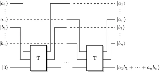
Matrix Vector Multiplication. The formula for matrix vector multiplication Ax calculates each element of the product vector b = (b1, . . . , bn) = (a11x1+a12x2+a1nxn, a21x1+a22x2+. . .+ a2nxn, . . . , an1x1+an2x2+. . .+annxn). To compute eachbiwe require at mostnproducts between the elements ofAand ofx. Therefore, the matrix-vector product requires at mostn2 products. It remains to show that the computation is reversible.
Figure 1 shows a reversible circuit for computing the inner product between two vectors. This is simply done by replacing the products by Toffoli gates. This quantum circuit is also itself reversible; applying the circuit twice leads to identity. In total, the inner product of twon-bit vectors can be computed, on a superposition of inputs, usingnToffoli gates. Therefore, the computation of such a matrix vector multiplication requires at mostn2 Toffoli gates.
|a1i
. . .
|ani
|b1i
. . .
|bni
|0i
T T
|a1i
. . .
|ani
|b1i
. . .
|bni
|a1b1+· · ·+anbni
. . .
Fig. 1.Computing the inner product on a superposition of inputs.
Matrix Multiplication. In the same fashion it is possible to compute matrix products in the quan-tum setting. Each column of the matrix can be computed using matrix vector multiplication, which, in turn, can be implemented using n2 Toffoli gates. In total, a reversible quantum circuit for computing matrix multiplication on a superposition of inputs requires at mostn3Toffoli gates, for square matrices.
Utilizing this quantum circuit for inner product between two vectors the quantum oracle for consistency checking can be constructed. Despite the fact that this naive quantum matrix multi-plication is computed inO(n3), time greater thanO(nω) whereω∼2.376 is the current classical complexity of matrix multiplication with the Coppersmith-Winograd algorithm, quantizing this computation will result in a lower quantum computational time for the classical MQ2 problem. ClassicalBooleanSolve, as well asSparseLinearSystemSolver and the provided subroutines are analyzed in the black box model, where matrix multiplication such as x→ Axfor a vector x and a matrix A are given by black boxes. We have provided the above construction to as-sure that such computations can be carried out by a quantum computer, reversibly and without entanglement concerns.
4
Complexity Analysis
We can now study the complexity ofQuantumBooleanSolve(Section 3.1). This analysis consists of constructing the quantum oracleQBSimplementing FF,kcons:{0,1}k→ {0,1}, which on inputa∈ Fk
For example, the quantization of the subroutineRandomSolwould consist of constructing a quan-tum circuitQRS.RandomSoltakes as input a matrixA∈Fn×n, a vectorb∈
Fn×1, a polynomial f(z) ∈ F[z] with f(0) 6= 0 (andL ⊂ F, which is in the case of MQ2 a field extention of F2. We would build
QRS :|a11i. . .|anni|f[0]−1i|f[1]i. . .|f[n]i|ri|w1i. . .|wni|b1i. . .|bni|0i. . .|0i → |a11i. . .|anni|f[0]−1i|f[1]i. . .|f[n]i|ri|w1i. . .|wni|b1i. . .|bni|0i. . .|0i|b01i. . .|b0ri|x1i. . .|xni|sAi
This quantum circuit takes as input the elements of the matrixA, the coefficients of the function f, the elements of the random vector w,r= deg(f), and the elements of the vector b, as well as wires for computation space, and returnsb0r=b+Aw,x=−Pn
i=1 f[i] f[0]A
i
rb0r, a booleansA which takes the value of 1 ifAx=b and 0 otherwise, along with the input for reversibility.
Theorem 5. The quantum circuit
QRS:|Ai|fi|wi|ri|bi|0i. . .|0i → |Ai|fi|wi|ri|bi|0i. . .|0i|b0i|xi|sAi
implementing RandomSolrequiresO(n3+ 2n2+ 3n+ 1) quantum gates to compute. In the
black-box model, when provided with an oracle to compute matrix-vector and matrix-matrix products,
QRS requiresO(r)evaluations of the black box, andO(nr) operations in the base fieldF, which is equivalent to the classical complexity ofRandomSol.
A proof of the above theorem is fairly straightforward when directly analyzing a quantum analogue of the classical algorithm provided above for RandomSol. It is clear that steps 4, 6, and 7 of RandomSol are the only steps computed by the QRS quantum circuit. Firstly, step 4 consists of the computation of b0r = (b01, . . . , br0) = b+Aw, the first r entries of the vector b0. This is merely matrix-vector multiplication and vector-vector addition; we compute the r entries of b0 withrnT gates for multiplication andrCNOT gates for addition, totalingO(rn+r)≤O(n2+n) quantum gates. In the black box model, we have 1 oracle query for matrix-vector multiplication and O(r) field operations for addition of two vectors. Secondly, step 6 consists of computing for i= 1. . . nthe matrix-vector product (A)·(Ai−1b0) withn2 T gates, followed by the computation of fi
f0 via one T-gate, and computing the ith term of the sum with an additional T gate. This is
O(n(n2+ 2) + 1) quantum gates to computexwhen we consider the additional NOT gate at the end of the computation. In the black box model, we haveO(n) black box matrix-vector product queries and O(nr) field operations for the sum. Finally, the equality test conducted in step 7 consists of computing the matrix-vector productAxwithn2 T gates, followed bynCNOT gates to compute, element by element, (Ax)i⊕bi, and then oneTn+1gate to compute the valuesA. In the black box model, this is 1 call to the matrix-vector product oracle. Therefore, we have established the equivalence of the classical complexity of the subroutineRandomSolwith the quantum oracle implementing the functionQRS in the black-box model.
Similar arguments demonstrate the equivalence of SparseLinearSystemSolver as well as the entire quantum circuit QBS. Due to the equivalence of the classical and quantum consistency checks in the black-box model, it is straightforward to adapt Theorem 2 toQuantumBooleanSolve, as follows.
Theorem 6. Let θ,2 ≤ θ ≤ 3 is such that any two n×n matrices can be multiplied in O(nθ)
operations in the underlying field. For any > 0, and α ≥ 1 and sufficiently large m = dαne, testing the consistency of all Macaulay matrices inQuantumBooleanSolve(m,n,k)requires the:
– evaluation of O(2(1−2γ+θFα(γ)+)n)quantum gates in the deterministic variant;
– evaluation, on average,O(2(1−2γ+2Fα(γ)+)n)quantum gates in the probabilistic variant,
where γ = 1− k
n, Fα(γ) = −γlog2(DD(1−D)(1−D)) with D = M( α
γ) and M(x) = −x+ 1 2 + 1
2 q
2x2−10x−1 + 2(x+ 2)p
The above complexity is obtained through the full evaluation of the cost of the consistency check oracle, QBS, which is equivalent to the cost of the classical consistency check in the black box model. The quantum circuit forQBScan then be run in superposition over all generated Macaulay matrices,P
a∈Fk
2|Mai. Amplitude amplification is then utilized, as in Grover’s algorithm, to
de-termine thea∈Fk
2 such thatMais inconsistent.
If we are guaranteed only one input a ∈Fk
2 is such that the generated Macaulay matrix Ma is
inconsistent, the algorithm requiresO(2k/2) =O(2((1−2γ)n) evaluations of the quantum circuitQBS implementingFcons
F,k forF∈F2[x1, . . . , xn]mas well as the diffusion gateDfor Grover’s algorithm. When we have more than onea∈F2such thatMais inconsistent, amplitude amplification must
be run
O π 4
s
2k
|a∈Fk
2 :Mainconsistent|
!
times to recover sucha∈Fk 2.
As in the classical analysis of ClassicalBooleanSolve, in the case that the Macaulay ma-trices are found to be inconsistent, the full system F may be consistent. We therefore must determine the remainder of the solution, once we have found a ∈ Fk
2 such that Ma is
in-consistent. This exhaustive search can be performed using Grover’s algorithm with a quantum oracle for the specialized system ˜Fa, where if a = (y1, . . . , yk) we have ˜F = ( ˜f1, . . . ,fm˜ ) = (f1(x1, . . . , xn−k, y1, . . . , yk), . . . , fm(x1, . . . , xn−k, y1, . . . , yk)). Similarly to the classical analysis, we find that an overwhelming amount of computational cost is the consistency check performed byQBS; the cost of the second exhaustive search, performed over the remaining n−kvariables, is negligible. By definition of strong semi-regularity, the number of such searches is bounded by O(2(1−2γ+2Fα(γ))n), and therefore the cost of the second exhaustive search is bounded by the cost
of the consistency check.
To derive the asymptotic complexity, we now minimize (for example, numerically) the exponents stated in Theorem 6.
Lemma 2. Let the notations be as in Theorem 6 and α= 1. Then, the function (1−2γ)+θFα(γ)
is bounded by:
– 0.477 = 1−0.523, whenθ= 3andγ= 0.1,
– 0.47 = 1−0.53, whenθ= 2.376 andγ= 0.13,
– 0.462 = 1−0.538, whenθ= 2andγ= 0.17
It can be remarked that the value ofθhas a minimal impact on the bounds provided in the Lemma below; less than in the classical setting (see Section 2.1). Note that these results can be extended to anyα≥1.
To assure the reader that such computations can be performed on a quantum computer, we have provided a naive matrix-vector and matrix-matrix product circuit computed via inner product in the previous section. Finally, in summary, we have:
Theorem 7. QuantumlBooleanSolveis correct and solvesMQ2. Ifm=n, then – for any >0 –
the deterministic variant of the algorithm requires to evaluateO(2(0.47+)n)quantum gates provided
that the system is0.13-strong semi-regular. The Las-Vegas probabilistic variant requires to evaluate an expected number ofO(2(0.462+)n)quantum gates if the system is0.17-strong semi-regular.
This theorem follows directly from the equivalence of the classical and quantum complexity of the consistency checks, as well as the above Lemma 2.
5
Acknowledgment
The first and last authors are partially supported by the french Programme d’Investissement d’Avenir under national project RISQ1 P1415807. Delaram Kahrobaei is partially supported by an ONR (Office of Naval Research) grant N00014-15-1-2164, as well as a PSC-CUNY grant from the CUNY Research Foundation. We also would like to thanks the referees of PKC’18 for their comments on the first version of this document.
References
1. Albrecht, M.R., Cid, C., Faug`ere, J., Fitzpatrick, R., Perret, L.: Algebraic algorithms for LWE prob-lems. IACR Cryptology ePrint Archive 2014, 1018 (2014),http://eprint.iacr.org/2014/1018 2. Arora, S., Ge, R.: New algorithms for learning in presence of errors. In: Aceto, L., Henzinger, M.,
Sgall, J. (eds.) Automata, Languages and Programming - 38th International Colloquium, ICALP 2011, Zurich, Switzerland, July 4-8, 2011, Proceedings, Part I. Lecture Notes in Computer Science, vol. 6755, pp. 403–415. Springer (2011),https://doi.org/10.1007/978-3-642-22006-7_34 3. Bardet, M., Faug`ere, J.C., Salvy, B., Spaenlehauer, P.J.: On the complexity of solving quadratic
boolean systems. Journal of Complexity 29(1), 53–75 (2013)
4. Bennett, C.H., Bernstein, E., Brassard, G., Vazirani, U.V.: Strengths and weaknesses of quantum com-puting. SIAM J. Comput. 26(5), 1510–1523 (1997),http://dx.doi.org/10.1137/S0097539796300933 5. Berbain, C., Gilbert, H., Patarin, J.: QUAD: A multivariate stream cipher with provable security. J.
Symb. Comput. 44(12), 1703–1723 (2009),http://dx.doi.org/10.1016/j.jsc.2008.10.004 6. Bernstein, D.J., Buchmann, J., Dahmen, E. (eds.): Post-quantum cryptography. Mathematics and
Statistics Springer-11649; ZDB-2-SMA, Springer Berlin Heidelberg, Berlin, Heidelberg (2009),http: //opac.inria.fr/record=b1128738
7. Bettale, L., Faug`ere, J.C., Perret, L.: Hybrid Approach for Solving Multivariate Systems over Finite Fields. Journal of Mathematical Cryptology 3(3), 177–197 (2010),http://www-salsa.lip6.fr/~jcf/ Papers/JMC2.pdf
8. Bettale, L., Faug`ere, J.C., Perret, L.: Solving Polynomial Systems over Finite Fields: Improved Analysis of the Hybrid Approach. In: Proceedings of the 37th International Symposium on Sym-bolic and Algebraic Computation. pp. 67–74. ISSAC ’12, ACM, New York, NY, USA (2012), http://www-polsys.lip6.fr/~jcf/Papers/FBP12.pdf
9. Bettale, L., Faug`ere, J.C., Perret, L.: Cryptanalysis of multivariate and odd-characteristic HFE vari-ants. pp. 441–458
10. Bouillaguet, C., Chen, H.C., Cheng, C.M., Chou, T., Niederhagen, R., Shamir, A., Yang, B.Y.: Fast exhaustive search for polynomial systems inf2. pp. 203–218
11. Brassard, G., Høyer, P., Mosca, M., Tapp, A.: Quantum amplitude amplification and estimation. In: Quantum computation and information (Washington, DC, 2000), Contemp. Math., vol. 305, pp. 53–74. Amer. Math. Soc., Providence, RI (2002),http://dx.doi.org/10.1090/conm/305/05215 12. Buchberger, B.: Bruno Buchberger’s PhD thesis 1965: An algorithm for finding the basis elements
of the residue class ring of a zero dimensional polynomial ideal. Journal of Symbolic Computation 41(3-4), 475–511 (2006)
13. Buchberger, B., Collins, G.E., Loos, R.G.K., Albrecht, R.: Computer algebra symbolic and algebraic computation. SIGSAM Bull. 16(4), 5–5 (1982)
14. Carlet, C., Hasan, M.A., Saraswat, V. (eds.): Security, Privacy, and Applied Cryptography Engineer-ing - 6th International Conference, SPACE 2016, Hyderabad, India, December 14-18, 2016, Proceed-ings, Lecture Notes in Computer Science, vol. 10076. Springer (2016), https://doi.org/10.1007/ 978-3-319-49445-6
15. Chen, L., Jordan, S., Liu, Y.K., Moody, D., Peralta, R., Perlner, R., Smith-Tone, D.: Report on post-quantum cryptography. Reasearch report NISTIR 8105, NIST (2003),http://csrc.nist.gov/ publications/drafts/nistir-8105/nistir_8105_draft.pdf
16. Chen, M., H¨ulsing, A., Rijneveld, J., Samardjiska, S., Schwabe, P.: From 5-pass MQ -based iden-tification to MQ based signatures. In: Cheon, J.H., Takagi, T. (eds.) Advances in Cryptology -ASIACRYPT 2016 - 22nd International Conference on the Theory and Application of Cryptology and Information Security, Hanoi, Vietnam, December 4-8, 2016, Proceedings, Part II. Lecture Notes in Computer Science, vol. 10032, pp. 135–165 (2016),https://doi.org/10.1007/978-3-662-53890-6_5 7
17. Chen, M.S., Hlsing, A., Rijneveld, J., Samardjiska, S., Schwabe, P.: Sofia: Mq-based signatures in the qrom. Cryptology ePrint Archive, Report 2017/680 (2017),http://eprint.iacr.org/2017/680 18. Faug`ere, J.C., Otmani, A., Perret, L., Tillich, J.P.: Algebraic Cryptanalysis of McEliece Variants with
Compact Keys. In: Proceedings of Eurocrypt 2010. Lecture Notes in Computer Science, vol. 6110, pp. 279–298. Springer Verlag (2010),http://www-salsa.lip6.fr/~jcf/Papers/Eurocrypt2010.pdf 19. Faug`ere, J.C., Perret, L., De Portzamparc, F.: Algebraic Attack against Variants of McEliece with
Goppa Polynomial of a Special Form. In: Advances in Cryptology Asiacrypt 2014. Kaohsiung, Tawan (Sep 2014),http://hal.inria.fr/hal-01064687
20. Faug`ere, J.C., Joux, A.: Algebraic cryptanalysis of hidden field equation (HFE) cryptosystems using gr¨obner bases. pp. 44–60
21. Gall, F.L.: Powers of tensors and fast matrix multiplication. In: Nabeshima, K., Nagasaka, K., Winkler, F., Sz´ant´o, ´A. (eds.) International Symposium on Symbolic and Algebraic Computation, ISSAC ’14, Kobe, Japan, July 23-25, 2014. pp. 296–303. ACM (2014),http://doi.acm.org/10.1145/2608628. 2608664
22. Garey, M.R., Johnson, D.S.: Computers and Intractability: A Guide to the Theory of NP-Completeness. W. H. Freeman (1979)
23. von zur Gathen, J., Gerhard, J.: Modern Computer Algebra (3. ed). Cambridge University Press (2013)
24. Giesbrecht, M., Lobo, A., Saunders, B.D.: Certifying inconsistency of sparse linear systems. In: Pro-ceedings of the 1998 international symposium on Symbolic and algebraic computation. pp. 113–119. ACM (1998)
25. Grover, L.K.: A fast quantum mechanical algorithm for database search. In: Proceedings of the twenty-eighth annual ACM symposium on Theory of computing. pp. 212–219. ACM (1996)
26. Ivanyos, G., Santha, M.: Solving systems of diagonal polynomial equations over finite fields. Theor. Comput. Sci. 657, 73–85 (2017),https://doi.org/10.1016/j.tcs.2016.04.045
27. Kipnis, A., Patarin, J., Goubin, L.: Unbalanced oil and vinegar signature schemes. pp. 206–222 28. Lokshtanov, D., Paturi, R., Tamaki, S., Williams, R., Yu, H.: Beating brute force for systems of
polynomial equations over finite fields, to appear, 27th ACM-SIAM Symposium on Discrete Algorithms (SODA 2017)
29. NIST: Proposed submission requirements and evaluation criteria for the post-quantum cryptogra-phy standardization process (DRAFT).,http://csrc.nist.gov/groups/ST/post-quantum-crypto/ documents/call-for-proposals-draft-aug-2016.pdf
30. Perret, L.: Bases de Gr¨obner en Cryptographie Post-Quantique. (Gr¨obner bases techniques in Quantum-Safe Cryptography) (2016),https://tel.archives-ouvertes.fr/tel-01417808
31. Westerbaan, B., Schwabe, P.: Solving binary mq with grover’s algorithm. In: Carlet, C.; Hasan, A.; Saraswat, V.(ed.), Security, Privacy, and Advanced Cryptography Engineering: 6th International Con-ference, SPACE 2016, Hyderabad, India, December 14-18, 2016. pp. 303–322. Berlin: Springer-Verlag (2016)