Article
1
Comparing Performance of Nonlinear Complexity
2
Metrics for Assessing Quality of ECGs Collected in
3
Real Time
4
Yatao Zhang 1,2,*, Hai Liu 2, Shoushui Wei 1 and Chengyu Liu 3
5
1 School of Control Science and Engineering, Shandong University, Jinan, China
6
2 School of Mechanical, Electrical & Information Engineering, Shandong University, Weihai, China
7
3 School of Instrument Science and Engineering, Southeast University, Nanjing, China
8
* Correspondence: [email protected]; Tel.: +86-187-6919-7261
9
Abstract: We compared performance of a novel encoding Lempel-Ziv complexity (ELZC) with
10
approximate entropy (ApEn), sample entropy (SmpEn) and permutation entropy (PerEn) as
11
nonlinear metric to assess ECG quality. Firstly to compare performance of discerning randomness
12
and inherent nonlinear properties within time series, this study calculated the aforementioned
13
four nonlinear complexity values on several typical artificial time series i.e., Gauss noise, two
14
kinds of noisy time series, two kinds of Logistic series and periodic series, respectively. Then for
15
analyzing sensitivity of the aforementioned four complexity methods to content level of different
16
types noise within ECG recordings, we investigated variation trend of ELZC, ApEn, SmpEn and
17
PerEn in several synthetic ECG recordings containing different types noise (i.e., baseline wander,
18
muscle artefacts, electrode motion, power line and mixed noise) and different signal noise ratios
19
(i.e., 15, 10, 5, 0, −5 and −10 dB). Finally, the four complexity methods were employed to classify
20
the quality of real ECG recordings from the PhysioNet/Computing in Cardiology Challenge 2011
21
(CINC 2011) of the MIT databases, then receiver operating characteristic curves (ROC) and their
22
corresponding area under curve (AUC) were yielded. The results showed ELZC could not only
23
distinguish randomness and chaotic within time series but also reflect content level of noise within
24
time series, and the highest AUC of PerEn, ELZC, SmpEn and ApEn were 0.850, 0.695, 0.474 and
25
0.461, respectively. The results demonstrated PerEn and ELZC were more effectively than ApEn
26
and SmpEn for assessing ECG quality.
27
Keywords: ECG quality assessment; complexity; entropy; ROC
28
29
1. Introduction
30
In practice, considerable amount of ECG recordings collected via wearable device and smart
31
phone cannot be used in clinic because their quality is so poor that their main waveform cannot be
32
identified, so ECG recordings in real time have to be classified their quality before diagnosis [1-3].
33
At present, most methods of assessing ECG quality employed time and frequency domain
34
features extracted from ECG recordings. Langley et al. [4] just relied on time domain features i.e.,
35
flat lines, saturation, baseline drift, high and low amplitude and steep slope, to assess quality of ECG
36
recordings, and the corresponding assessment accuracy was 85.7% on test data. Similarly Kužílek et
37
al. [5] summarized six waveform rules to assess ECG quality and obtain 83.6% on test data. In most
38
cases, waveform features are easy to be identified and calculated, however an assessing quality
39
method has poor generation ability when it just relies on waveform features. Frequency domain
40
features i.e., power spectrum density (PSD) can reflect energy distribution within time series, so it
41
helps to extract some detailed inherent information from physiological series. So PSD was usually
42
used for assessing quality of ECG recordings [6-8]. In [6], Zaunseder et al. proposed an assessment
43
method based on thirty five frequency domain features generated from PSD, and assessment result
44
of the method was 90.4% and higher than that of the other methods just based on time domain
45
features. In fact some ECG recordings can be classified as unacceptable signals by some obvious
46
waveform features i.e., flat line and high amplitude. So some assessment methods combining
47
waveform features with frequency features not only improve assessment accuracy but also help for
48
calculation efficiency. Clifford et al. [7] and Zhang et al. [8] proposed an assessing method based on
49
combination of time and frequency features, respectively. Comparing with the previous methods,
50
the combination methods of multi features can provide relatively more comprehensive information
51
within the ECG recordings. However, the methods are difficult to further improve their
52
classification accuracy, and their generation ability also needs to be improved. So it is necessary to
53
find new features that can reflect the inherent nature of physiological series. Actually nature of ECG
54
signal is nonlinear, so nonlinear complexity approaches can be used for extracting the inherent
55
nonlinear properties of ECG recordings to assess quality of ECG signals [8, 9]. Some nonlinear
56
complexity approaches i.e., classical Lempel-Ziv complexity (CLZC), approximate entropy (ApEn),
57
sample entropy (SmpEn) and permutation entropy (PerEn) have been extensively used for
58
biomedical signal analysis [10-13]. Zhang et al. [14] evaluated performance of CLZC on ECG quality
59
assessment and concluded that the CLZC was only sensitive to high frequency noise. However in
60
practice ECG signals are usually contaminated by the mixed noise including high frequency, low
61
frequency and power line noise, so performance of CLZC is not satisfactory when it is used as
62
quality assessment metric. In addition, the ApEn, SmpEn and PerEn has been not yet reported to be
63
used for assessing ECG quality. Zhang et al. [15] proposed an encoding Lempel-Ziv complexity
64
(ELZC) to analyze the nonlinear complexity of physiological signal, and the approach can better
65
discern random and chaotic character within time series than other LZ complexity approaches. In
66
this study, we compared the ELZC with ApEn, SmpEn and PerEn as quality metric for assessing
67
ECG quality.
68
In this study, we firstly calculate ELZC, ApEn, SmpEn and PerEn of six typical artificial time
69
series i.e., Gauss noise, two kinds of noisy series contained different level of noise, two kinds of
70
Logistic series (different μ) and periodic series so as to comparing performance of the four
71
complexity methods for discerning randomness and the inherent nonlinear properties within time
72
series. Then we calculated the four aforementioned complexity values on artificial synthetic ECG
73
signals with different types noise (i.e., baseline wander (BW), muscle artefacts (MA), electrode
74
motion (EM), power line (PL) and mixed noise) and Signal to Noise Ratio (SNR) so as to not only
75
analyze the four complexity methods whether can reflect different types of noise, but also evaluate
76
sensitivity of the four methods to noise content level of the artificial synthetic ECG signals. Finally
77
we used the ELZC, ApEn, SmpEn and PerEn on real ECG recordings for assessing quality by by
78
receiver operating characteristic curve (ROC) and the corresponding area under curve (AUC). The
79
study is organized as follows: Section 2 describes the four complexity methods and dataset
80
including artificial time series and real ECG signals. The experimental results and discusses are
81
described in Section 3. Section 4 concludes the current study.
82
2. Materials and Methods
83
2.1. Artificial synthetic and Real ECG siginals
84
For presenting comprehensive study, we used three types of datasets including six typical
85
artificial time series, the artificial synthetic ECG recordings and the real ECG recordings from the
86
MIT database of the PhysioNet/Computing in Cardiology Challenge 2011 (CinC 2011).
87
First, six typical artificial time series were employed in this study. Gau noise represented a
88
pure noise, MIX(0.4) means that 40 percent of a period series of length N were randomly chosen and
89
replaced with independent identically distributed random noise, and it was used as a mixed noise
90
series, MIX(0.2) was similar. Logistic (Logi) mapping series represent nonlinear series and are
91
defined as
92
1 (1 )
n n n
x+ = × × −μ x x , (1)
where 1<μ≤4. In this study, Logi(4.0) represented the Logistic series that μ were set as 4.0, and
93
Logi(3.8) was similar. Logi(3.5) was defined as the same way and represented the periodic series.
Second, in this study, we used 48 real ECG recordings from the MIT arrhythmia database and
95
the real common noises within ECG signals from the MIT Noise Stress Test Database (NSTDB) to
96
construct the artificial synthetic noisy ECG recordings [16-18]. The 48 arrhythmia ECG recordings
97
collected from the real clinical environment, each with duration of 30 mins and a sample rate of 360
98
Hz. Baseline correction was performed for removing the main BW noise because the noise contained
99
in the raw signals affected the content level of BW noise within ECG recordings leading to inaccurate
100
results in further study. The NSTDB provides three common noises that can be typically found in
101
real clinical application, i.e., MA, EM and BW. In addition, another common noise existed in several
102
clinic environments i.e., PL was also used to combine the artificial synthetic ECG recordings.
103
SNR reflects the content level of noise within signal, and SNR is defined as
104
10
10 log ( signal )
noise
P
SNR= × P , (2)
where Psignal and Pnoise denote the power of the clean ECG and the power of the noise, respectively.
105
Five kinds of synthetic noisy ECG signal, i.e., the real ECG plus BW, EM, MA, PL and hybrid
106
noise, respectively, were employed for calculating sensitivity of the ELZC on different SNR in this
107
study. In practice, ECG signals usually cannot be used for clinical purpose when SNR of the signals
108
lower than -10 dB because the main waveform of ECG signals cannot be recognized due to a lot of
109
noise. So the range of SNR of the four synthetic ECG signals is from -10 dB to 15 dB. For each SNR
110
level, 48 repeats were yielded and the mean value and standard deviation of each type signal were
111
calculated in this study. In fact, ECG signals are usually contaminated by a mixed noise instead of
112
one of the aforementioned noises i.e., BW, EM, MA and PL noise. Thus we built the hybrid noise and
113
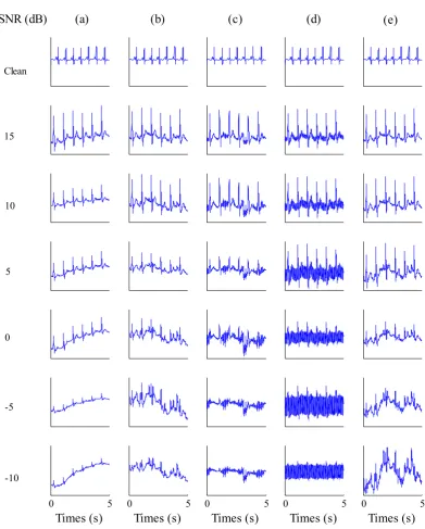
added to the real ECG recordings, with the same proportion (25%) for each noise type.Figure 1
114
shows the aforementioned five artificial noisy ECG signals with SNR from -10 dB to 15 dB with steps
115
of 5 dB.
116
Third, the real data from CinC 2011 [2] consisted of training set in this study. Training set
117
includes 1000 12-lead ECG recordings, and it is recordings open to all researchers and given quality
118
label as ‘acceptable’ or ‘unacceptable’. In training set, each recording lasts for 10s. The ECG
119
recordings with lead-fall is no need to calculated their complexity because waveforms of the
120
recordings look like a straight line so that the recordings are easy to be identified, and assessment
121
accuracy is also effected by the recordings with lead-fall. So this study first removed the ECG
122
recordings with lead-fall in training set, and then the remained ECG signals included 767 acceptable
123
and 95 unacceptable ECG signals.
0 5
Times (s)
0 5
Times (s)
0 5
Times (s)
0 5
Times (s)
0 5
Times (s)
1510
5
0
-5
-10 Clean
SNR (dB)
(a)
(b)
(c)
(d)
(e)
125
Figure 1. The real ECG recordings and the artificial synthetic noisy ECG recordings with SNR from
126
-10 to 15 dB: (a) The real and the clean plus BW noise; (b) The real and the clean plus EM; (c) The real
127
and the clean plus MA; (d) The real and the clean plus PL and (e) The real and the clean plus mixed
128
noise.
129
2.2. Encoding Lempel-Ziv complexity (ELZC)
130
The classical LZ complexity consists of two steps. Firstly, an original time series is transformed
131
into a new binary symbolic sequence by comparing with the mean or median of the original series,
132
and then the LZ value from the binary sequence is calculated. In this study, the original series was
133
transformed into an 8-state symbolic (3-bit binary) sequence by an encoding way.
134
Each xi within the original signal X=x1, x2, …, xn is transformed into a 3-bit binary symbol
135
Step 1, the b1(i) is determined by comparing xi with the mean of signal X, and b1(i) is set 0 when
137
the xi is less than the mean, otherwise the b1(i) is 1.
138
Step 2, the b2(i) is 0 when the difference between xi and xi-1 is less than 0, otherwise the b2(i) is set
139
to 1. Initially,b2(1) is set to 0.
140
Step 3, calculated process of the third digit b3(i) is relatively complex, a variable Flag is first
141
denoted as follows:
142
1
1
0
( ) , 2,3,...,
1
i i
i i
if x x dm
Flag i i n
if x x dm
−
−
− <
= =
− ≥
, (3)
143
where dm is the mean distance between adjacent points within signal X. Subsequently, b3(i) is
144
calculated as follows:
145
3( ) ( ( ) 2 ( )), 2,3,...,
b i =NOT b i XOR Flag i i= n, (4)
where b3(i) is 0.
146
After the symbolic process, the LZ value of the new symbolic sequence will be calculated, and
147
the detailed calculation process is detail in [15]. In fact, the LZ complexity counter c(n) is closed
148
related to the new subsequence of consecutive characters within the symbolic sequence. For
149
calculating the counter c(n), the symbolic sequence B is scanned from left to right and the c(n) is
150
increased one unit when a new subsequence is encountered. First, S and Q are represented two
151
subsequences of B respectively, and SQ is the concatenation of S and Q. The subsequence SQπ
152
yielded from SQ after its last character is deleted (πis the operation deleting the last character in a
153
sequence). v(SQπ) is the vocabulary of all subsequences of SQπ. Initially, c(n)=1, S=s(1) and Q=s(2),
154
then SQπ=s(1). Generally, S=s(1), s(2), s(3), …, s(r) and Q=s(r+1), and so SQπ=S. Q is a subsequence
155
of SQπinstead of a new sequence when itbelongs tov(SQπ). Then Q is replaced with s(r+1), s(r+2) and
156
used to judge if it belongs to v(SQπ) or not. The aforementioned processes are repeat until Q= s(r+1),
157
s(r+2), …, s(r+i) and it is a new sequence instead of a subsequence of SQπ, then c(n)=c(n)+1.
158
Thereafter S=s(1), s(2), …, s(r+i) and Q=s(r+i+1). This above procedure is repeated until Q is the last
159
character of B. in fact the LZ complexity counter c(n) may be normalized as the C(n)
160
log ( )
( ) ( ) n
C n c n
n
α
= , (5)
where n is the length of signal X, α is the number of possible symbols contained in the new sequence.
161
Generally, the normalized complexity C(n) is consider instead of c(n) in practice.
162
2.3. ApEn, SmpEn and PerEn
163
• ApEn and SmpEn
164
Pincus proposed ApEn as a metric to quantified regularity of a time series [19], and it means
165
the probability of new pattern within time series when the dimension increases from m to m+1. The
166
process of calculating ApEn is described as follows: Let S be a time series of length N and S= s1, ...,
167
sN, and reconstruct a vector xi of the embedded dimension m and xi= si, si+1, si+2, …, si+m-1 for 1≤ i≤
168
N-m+1 where m indicates the embedding dimension. The distance dij between the two vectors xi and
169
xjis calculated where 1≤ i, j≤ N-m+1.
170
max ( ) ( ) , 0,1,..., 1
i j
d = s i k+ −s j k+ k= m− , (6)
For each vector xi, the number of the distance dij within r×SD is found where SD is the standard
171
deviation of the time series S, and the ratio of the number to the total number of vector N-m+1 is
172
calculated as Cim(r).
173
1 { }, 1, 2,..., 1
1
m
i i j
C num d r i N m
N m
= < = − +
Then the average degree of similarity for all of i is defined as
174
( )
1( )
1 1 ln 1 N m m m i i
r C r
N m
− +
=
Φ =
− +
, (8)Similarly, when the embedded dimension is m+1, the corresponding Cim+1(r) and φm+1(r) can be
175
obtained.
176
1 1 { }, 1, 2,...,
m
i i j
C num d r i N m
N m
+ = < = −
− , (9)
( )
( )
1 1 1 1 ln N m m m i ir C r
N m
−
+ +
=
Φ =
−
, (10)Then, the ApEn is described as follows:
177
1
lim[ m( ) m ( )]
N
ApEn r + r
→∞
= Φ − Φ , (11)
In fact, the length N is not infinite, so the ApEn can be calculated by Eq. 12 when N is a finite
178
number.179
1 ( ) ( ) m mApEn= Φ r − Φ + r , (12)
In fact, the SmpEn is a modified complexity method based on ApEn. Comparing with ApEn,
180
the SmpEn does not include self-similar patterns, and it also does not depend on data size. Finally
181
the SmpEn can be given as
182
1
ln[ m ( ) / m( )]
SmpEn= − B + r B r , (13)
where Bm(r) is the probability that two m-dimension vectors will match, and similarly Bm+1(r) is the
183
probability that two m+1 dimension vectors will match, and m is the embedding dimension[20].
184
In this study, both of ApEn and SmpEn were calculated with r as 0.15×SD where SD was the
185
standard deviation of the data series S, and m as 2.
186
• PerEn
187
The PerEn algorithm was detailed in [21-24]. A time series {si, i = 1,2, …, n} firstly is
188
reconstructed to generate the following matrix in phase space
189
1 1 1 ( 1)
1
( 1)
( 1)
m
i i i m i
k k k m k
s s s
S
s s s
S
s s s
S τ τ τ τ τ τ + + − + + − + + − = , (14)
where m is the embedding dimension and τ is delay time, and k=n-(m-1)×τ. Each a row of the matrix
190
represents a reconstructed component, so there are a total number of k reconstruction components
191
in the matrix. The ith reconstructed component Si contained m number of real values can be
192
arranged in an increasing order as
193
1 2
( 1) ( 1) ( m 1)
i j i j i j
s+ − τ ≤s+ − τ≤s+ − τ. (15)
If there exists two or more reconstructed components are equal, e.g. xi+(j1-1)τ=xi+(jm-1)τ, they can be
194
sorted according to the values of j1 and j2, that is, xi+(j1-1)τ<<xi+(j2-1)τwhen j1<j2. Accordingly, each of
195
reconstructed components can be transformed into a symbol series as
196
1 2
l m
S = j j j , (16)
where l=1, 2, …, k and k<<m!, and m! is the largest number of distinct symbols. The symbol sequence
197
Sl is one kind of arrangement that is mapped onto the m number symbols (j1, j2, …, jm). If the
probability of the occurrence of each symbol sequence is p1, p2, …, pk, respectively, the PE of k kinds
199
of different symbol sequences of time series si in terms of Shannon entropy can be defined as [24]:
200
( ) k ln
p l l
l
H m = −
p p , (17)When all the symbol sequences have the same probability namely pl=1/m!, Hp(m) can generate
201
the maximum value ln(m!). Finally Hp(m) can be normalized as [24]:
202
0≤Hp=Hp/ ln( !) 1m ≤ , (18)
The value of Hp represents the randomness degree of the time series si, and it described local
203
order structure of the time series. The smaller the value of Hp, the more regular and inerratic the
204
time series is. The change of Hp can reflect and magnify the minute details of the time series [21].
205
2.4. Testing performance of ELZC, ApEn, SmpEn and PerEn for discerning randomness and nonlinear
206
properties within time series
207
In fact, a good quality metric should be able to discern randomness and the inherent nonlinear
208
within physiological signals instead of confusing because physiological signal are nonlinear time
209
series instead of random series. ELZC has a satisfied performance on discerning randomness and
210
nonlinear properties within time series [15]. For comparing performance of the four aforementioned
211
complexity methods, this test was designed to calculate ELZC, ApEn, SmpEn and PerEn on six
212
typical artificial time series mentioned in Section 2.1. In this test, 20 samples for each type of series
213
were employed, and length of each sample was 100, 500 and 2000 points.
214
2.4. Analyzing sensitivity of ELZC, ApEn, SmpEn and PerEn to different types noise and different SNR
215
In ECG quality assessment, a satisfied quality metric should be able to reflect different types
216
and content level of noise within physiological series, meaning the metric is sensitive to different
217
SNR of signal. Aiming to evaluate sensitivity of ELZC to noise levels of ECG signals, we compared
218
ELZC, ApEn, SmpEn and PerEn values of the aforementioned synthetic noisy ECG signals in
219
Section 2.1 i.e., the real ECG signals plus BW, EM, MA, PL and hybrid noise, respectively. In this test,
220
50 samples for each type of synthetic ECG signals were used.
221
2.5. Using Receiver Operating Characteristic (ROC) Curve to verify classification performance of ELZC,
222
ApEn, SmpEn and PerEn
223
In this test, we calculated sensitivity (Se) and specificity (Sp) of the ApEn, SmpEn, PerEn and
224
ELZC methods on all leads of the real ECG recordings for generating ROC curve to compare
225
classification performance of the aforementioned nonlinear methods. For getting Se and Sp, we
226
calculated ELZC of each lead of the real 12-lead ECG recordings from the training set A of the CinC
227
2011, and the thresholds were selected from 0 to 1 in steps of 0.005. An ECG recordings was marked
228
as unacceptable when its ELZC value was higher than these threshes, otherwise it was recognized
229
as an acceptable recording. For comparing assessement performance with ELZC, we also calculated
230
the Sp and Se of ApEn, SmpEn and PerEn using the same method in this test. The two indexes Se
231
and Sp are usually used for evaluating classification results, and the two concepts are described as
232
follows:
233
/
/
Se true positive total number of unacceptable ECG recordings Sp true negative total number of acceptable ECG recordings
=
= , (19)
where true positive is number of identified unacceptable recordings among the unacceptable ECG
234
recordings, and ture negative is number of identified acceptable recordings among the acceptable
235
ECG recordings. Actually in this study normalization of data was necessary because the range of
236
values obtained by the aforementioned methods (i.e., ApEn, SmpEn, PerEn and ELZC) was
different, so the Min-Max normalization approach was employed to normalize the data in this
238
study. The approach is described as follows:
239
min( ) *
max( ) min( )
x x
x
x x
− =
− , (20)
where x and x* are an original time series and the new series after normalizing respectively.
240
3. Results and Discussions
241
3.1. Results of discerning randomness and nonlinear properties within time series
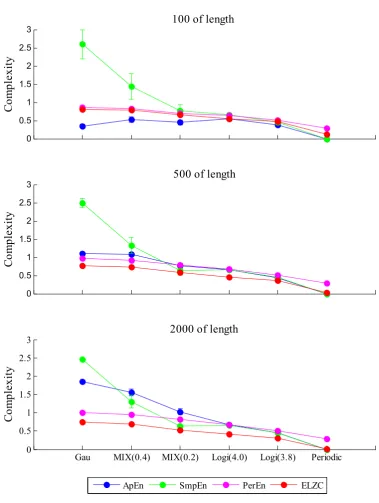
242
Figure 2 shows ApEn, SmpEn, PerEn and ELZC values of six aforementioned artificial time
243
series including Gau, MIX(0.4), MIX(0.2), Logi(4.0), Logi(3.8) and periodic series on three time
244
lengths 100, 500 and 2000, respectively. The PerEn and ELZC values exhibit monotonically decrease
245
in order of Gau, MIX(0.4), MIX(0.2), Logi(4.0), Logi(3.8) and periodic series on all type time lengths.
246
The ApEn values exhibit fluctuations on MIX(0.2) and Logi(4.0) when time length is 100, and
247
monotonically decrease in aforementioned order on 500 and 2000 length. Figure 2 shows the SmpEn
248
values monotonically decrease in aforementioned order on 100 of time length, and exhibits
249
fluctuations on MIX(0.2) and Logi(4.0) when time lengths are 500 and 2000 points respectively. The
250
results indicated the ELZC and PerEn approaches had better performance for discerning
251
randomness and nonlinear properties within time series on all type time lengths than ApEn and
252
SmpEn. In fact Both of ELZC and PerEn do not be performed on the original time series to calculate
253
complexity values. The ELZC approach employs firstly the encoding coarse grain method to
254
transform the original series into a new symbolic sequence then to calculate its complexity values.
255
Similarly PerEn calculates complexity values of a symbolic sequence generated from a
256
reconstructed matrix instead of the original series. For the ELZC and PerEn approaches, the
257
symbolic sequence can reflect properly nonlinear properties within time series instead of
258
randomness because the symbolic process preserves the inherent properties within the original
259
series, losing random component i.e., noise and unexpected components. Random components
260
within the original series affect calculation accuracy of ApEn and SmpEn approaches when the two
261
approaches are performed on the original time series.
0 0.5 1 1.5 2 2.5 3
C
om
pl
ex
ity
100 of length
0 0.5 1 1.5 2 2.5 3
Co
m
pl
ex
it
y
500 of length
Gau MIX(0.4) MIX(0.2) Logi(4.0) Logi(3.8) Periodic
0 0.5 1 1.5 2 2.5 3
Co
m
pl
ex
it
y
2000 of length
ApEn SmpEn PerEn ELZC
263
Figure 2. The ApEn, SmpEn, PerEn and ELZC Values of six typical artificial series on 100, 500 and
264
2000 time length, respectively
265
3.2. Results of sensitivity analysis
266
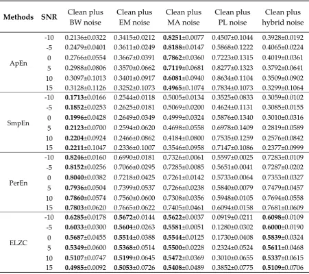
Table 1 shows the ELZC, ApEn, SmpEn and PerEn values for five artificial signals i.e., the
267
clean ECG plus BW, the clean plus EM, the clean plus MA, the clean plus PL and the clean plus
268
hybrid noise on several SNR from -10 to 15 dB, in steps of 5 dB. Table 1 shows ELZC values of all
269
synthetic ECG except that of the clean ECG plus PL noise exhibit monotonically decreasing with
270
increase of SNR. ApEn values of the clean ECG plus MA noise yield monotonically decreasing with
271
increase of SNR but those of other synthetic ECG signals are not. SmpEn and PerEn values of the
272
clean ECG plus BW noise exhibit monotonically decreasing with increase of SNR but those of other
273
synthetic ECG signals are not. In fact the clean ECG should be nonlinear signal instead of random
274
signal, so randomness within the clean ECG mixed several types noise i.e., BW, EM, MA and the
hybrid noise should increase with decreasing in SNR. The change trend of ELZC values, namely
276
decreasing with increasing in SNR, because nonlinear properties within ECG signals are more
277
obviously with SNR increasing instead of randomness. Table 1 shows the ELZC values of the clean
278
plus PL is 0.0919 when SNR is -10 dB, and the ELZC values increase with increasing of SNR.
279
Complexity of pure PL noise is nearly zero because PL is periodic signal, so complexity of the clean
280
ECG recordings plus PL noise should be higher than that of periodic signal. Furthermore in contrast
281
to complexity of the periodic signal, that of the clean plus PL noise should increase with the
282
increase of SNR because nonlinear properties within the signal increases.
283
Table 1. The ELZC values for clean ECG plus BW, EM, MA and mixed noise on several SNR from
284
-10 to 15 dB with steps of 5 dB.
285
Methods SNR Clean plus
BW noise
Clean plus EM noise
Clean plus MA noise
Clean plus PL noise
Clean plus hybrid noise
ApEn
-10 0.2136±0.0322 0.3415±0.0212 0.8251±0.0077 0.4507±0.1044 0.3928±0.0192 -5 0.2479±0.0401 0.3611±0.0249 0.8188±0.0147 0.5868±0.1222 0.4065±0.0224 0 0.2766±0.0554 0.3667±0.0391 0.7862±0.0360 0.7223±0.1315 0.4019±0.0361 5 0.2988±0.0806 0.3570±0.0662 0.7119±0.0681 0.8277±0.1323 0.3792±0.0641 10 0.3097±0.1013 0.3401±0.0917 0.6081±0.0940 0.8634±0.1104 0.3509±0.0902 15 0.3128±0.1126 0.3252±0.1073 0.4965±0.1074 0.7834±0.1073 0.3299±0.1064
SmpEn
-10 0.1713±0.0166 0.2544±0.0118 0.5005±0.0134 0.3525±0.0833 0.3059±0.0102 -5 0.1852±0.0253 0.2625±0.0181 0.5069±0.0200 0.4624±0.1131 0.3085±0.0155 0 0.1996±0.0428 0.2649±0.0349 0.4999±0.0324 0.5876±0.1340 0.3010±0.0316 5 0.2123±0.0700 0.2594±0.0620 0.4698±0.0558 0.6978±0.1409 0.2819±0.0589 10 0.2204±0.0924 0.2466±0.0862 0.4184±0.0800 0.7535±0.1259 0.2576±0.0842 15 0.2211±0.1047 0.2336±0.1007 0.3546±0.0958 0.7147±0.1086 0.2377±0.0999
PerEn
-10 0.8246±0.0160 0.6990±0.0181 0.7326±0.0061 0.5597±0.0025 0.7283±0.0109 -5 0.8152±0.0256 0.7066±0.0295 0.7285±0.0085 0.5651±0.0041 0.7287±0.0202 0 0.8040±0.0382 0.7218±0.0425 0.7261±0.0142 0.5733±0.0064 0.7353±0.0327 5 0.7936±0.0504 0.7399±0.0537 0.7266±0.0238 0.5840±0.0079 0.7479±0.0457 10 0.7860±0.0574 0.7560±0.0600 0.7308±0.0356 0.5948±0.0105 0.7694±0.0558 15 0.7803±0.0620 0.7665±0.0622 0.7405±0.0461 0.6094±0.0158 0.7681±0.0609
ELZC
-10 0.6285±0.0178 0.5672±0.0144 0.5622±0.0037 0.0919±0.0211 0.6098±0.0109 -5 0.6033±0.0300 0.5604±0.0263 0.5581±0.0051 0.1280±0.0302 0.6000±0.0190
0 0.5687±0.0455 0.5514±0.0388 0.5544±0.0125 0.1730±0.0408 0.5839±0.0324 5 0.5349±0.0600 0.5368±0.0514 0.5500±0.0228 0.2324±0.0524 0.5611±0.0468 10 0.5107±0.0747 0.5199±0.0645 0.5472±0.0369 0.3010±0.0655 0.5337±0.0615 15 0.4985±0.0092 0.5053±0.0726 0.5408±0.0489 0.3852±0.0775 0.5109±0.0706
3.3. ROC of the ELZC on real data
286
Figure 3 shows ROC curves and its corresponding area under the ROC curve on each lead of
287
the 12-lead ECG recordings. Figure 3 shows the ROC curves of ApEn and SmpEn on all leads of
288
12-lead ECG recordings are relatively overlap and lower than the ROC curves of PerEn and ELZC,
289
so the corresponding AUCs of ApEn and SmpEn are also relatively smaller than that of PerEn and
290
ELZC. Figure 3 shows that the PerEn generates the highest ROC curves, so it obtains the largest
291
AUCs on leads I, II, III, aVR, aVF, aVL, V1 and V2 that are 0.824, 0.744, 0.675, 0.850, 0.647, 0.736,
292
0.647 and 0.662, respectively. The ELZC generates the second highest ROC curves on the
293
aforementioned 8 leads, and Figure 3 also shows it obtains the second largest AUCs on
aforementioned leads. In fact the ELZC can also get the largest AUCs of 0.609, 0.336, 0.695 and 0.532
295
on leads V3, V4, V5 and V6, respectively.
296
PerEn and ELZC have relatively larger AUCs for classifying physiological series quality,
297
especially PerEn, because the PerEn and ELZC have a satisfied performance to distinguish
298
randomness and the inherent nonlinear properties within time series. Conversely, the ApEn and
299
SmpEn keep smaller AUCs so that the two complexity methods cannot effectively classify quality of
300
physiological series because they cannot discern accurately randomness and chaotic within time
301
series. In practice, many other factors cause yield poor quality of physiological series except the
302
lower SNR. For example poor electrode contact can cause poor quality of physiological time series
303
so that the main waveform of the series cannot be recognized. However these physiological series
304
are not contaminated by noise, so the series keep higher SNR. Additional, some unacceptable time
305
series have lower SNR because noise, however the time series keep a quasi-periodic property, so
306
that complexity of the series keeps a relatively lower level. This reason cause that classification
307
performance of ELZC is relatively lower than that of PerEn.
308
0 0.5
1 I II III
0 0.5
1 aVR aVF aVL
0 0.5
1 V1 V2
V3
0 0.5 1 0
0.5
1 V4
0 0.5 1
V5
0 0.5 1
V6
ELZC ApEn SmpEn PerEn ELZC:0.614
ApEn:0.426 SmpEn:0.419 PerEn:0.824
ELZC:0.587 ApEn:0.461 SmpEn:0.474 PerEn:0.744
ELZC:0.576 ApEn:0.436 SmpEn:0.459 PerEn:0.850
ELZC:0.336 ApEn:0.334 SmpEn:0.305 PerEn:0.333
ELZC:0.695 ApEn:0.416 SmpEn:0.410 PerEn:0.669
ELZC:0.587 ApEn:0.349 SmpEn:0.347 PerEn:0.675
ELZC:0.541 ApEn:0.396 SmpEn:0.454 PerEn:0.647
ELZC:0.519 ApEn:0.352 SmpEn:0.417 PerEn:0.736
ELZC:0.556 ApEn:0.273 SmpEn:0.251 PerEn:0.647
ELZC:0.541 ApEn:0.306 SmpEn:0.280 PerEn:0.662
ELZC:0.609 ApEn:0.365 SmpEn:0.332 PerEn:0.582
ELZC:0.532 ApEn:0.324 SmpEn:0.296 PerEn:0.486
AUC AUC
AUC
309
Figure 3. ROC curve of the ApEn, SmpEn, PerEn and ELZC on all leads i.e., I, II, III, aVR, aVF, aVL,
310
V1, V2, V3, V4, V5 and V6, respectively, and its corresponding AUC.
311
4. Conclusions
312
In this study, we compared a novel ELZC complexity method with ApEn, SmpEn and PerEn
313
for ECG quality assessment. The experiment results indicate that ELZC and PerEn have satisfied
314
performance for distinguishing randomness and inherent nonlinear properties within time series,
315
and ELZC can efficiently reflect types of noise and content level of noise contained in physiological
316
signal because the ELZC values of the synthetic noisy signals decrease monotonically with increase
of SNR except that of the clean ECG plus PL noise. The experiment results on real ECG recordings
318
indicate that the ELZC and PerEn are a satisfied quality metric for assessing quality of physiological
319
series. In practice, the ELZC and PerEn metirc have to be combined with the other quality metrics
320
i.e., waveform and frequency metrics for physiological signal quality assessment.
321
Acknowledgments: Project supported by the China Postdoctoral Science Foundation (No. 2017M612280), the
322
National Natural Science Foundation of China (No. 61473174), and the Natural Science Foundation of
323
Shandong Province, China (No. ZR2015AM015). We would like to thank the MIT PhysioNet for providing the
324
open source code of PerEn and Cardiology Challenge database.
325
Conflicts of Interest: The author declares no conflict of interest.
326
327
References
328
1. Clifford, G.D.; Moody, G.B. Signal quality in cardiorespiratory monitoring. Physiological Measurement 2012,
329
33, E01.
330
2. Moody, G.B. Physionet/computing in cardiology challenge 2011, July 2011. URL: http:// physionet.org /
331
challenge/ 2011.
332
3. Li, Q.; Clifford, G.D. Signal quality and data fusion for false alarm reduction in the intensive care unit.
333
Journal of Electrocardiology 2012, 45, 596-603.
334
4. Langley, P.; Di Marco, L.Y.; King, S.; Duncan, D.; Di Maria, C.; Duan, W.; Bojarnejad, M.; Zheng, D.; Allen,
335
J.; Murray, A. An algorithm for assessment of quality of ECGs acquired via mobile telephones, Proc. of the
336
38th Computing in Cardiology, Hangzhou, China, 2011, 281-284.
337
5. Kužílek, J.; Huptych, M.; Chudáček, V.; Spilka, J.; Lhotská, L. Data driven approach to ECG signal quality
338
assessment using multistep SVM classification, Proc. of the 38th Computing in Cardiology, Hangzhou,
339
China, 2011, 453-455.
340
6. Zaunseder, S.; Huhle, R.; and Malberg, H. Assessing the usability of ECG by ensemble decision trees. Proc.
341
of the 38th Computing in Cardiology, Hangzhou, China, 2011, 277-280.
342
7. Clifford, G.D.; Behar, J.; Li, Q.; Rezek, I. Signal quality indices and data fusion for determining clinical
343
acceptability of electrocardiograms. Physiological Measurement 2012, 33, 1419-1434.
344
8. Zhang, Y.T.; Liu, C.Y.; Wei, S.S.; Wei, C.Z.; Liu, F.F. ECG quality assessment using a kernel support vector
345
machine and genetic algorithm with a feature matrix. Journal of Zhejiang University-SCIENCE C (Compute &
346
Electron) 2014, 15, 564-573.
347
9. Arfan Jaffar, M.; Hussain A.; Mirza, Anwar M. Fuzzy Entropy and Morphology based fully automated
348
segmentation of lungs from CT scan images. International Journal of Innovative Computing, Information and
349
Control 2009, 5, 4993-5002.
350
10. Lempel, A., Ziv, J. On the complexity of finite sequences. IEEE Trans Inf Theory 1976, 22, 75-81.
351
11. Balasubramanian, K.; Nair, S.S.; Nagaraj, N. Classification of periodic, chaotic and random sequences
352
using approximate entropy and Lempel-Ziv complexity measures. Pramana 2015, 84, 365-372.
353
12. Yentes, J.M.; Hunt, N.; Schmid, K.K.; Kaipust, J.P.; McGrath, D.; Stergiou, N. The appropriate use of
354
approximate entropy and sample entropy with short data sets. Annals of biomedical engineering 2013, 41,
355
349-365.
356
13. Ravelo-García, A. G.; Navarro-Mesa, J. L.; Casanova-Blancas, U.; Martin-Gonzalez, S.; Quintana-Morales,
357
P.; Guerra-Moreno, I.; Canino-Rodríguez, José M.; Hernández-Pérez, E. Application of the permutation
358
entropy over the heart rate variability for the improvement of electrocardiogram-based sleep breathing
359
pause detection. Entropy 2015, 17, 914-927.
360
14. Zhang, Y.T.; Wei, S.S.; Di Maria, C.; Liu, C.Y. Using Lempel-Ziv Complexity to Assess ECG Signal Quality.
361
Journal of Medical and Biological Engineering 2016, 36, 625-634.
362
15. Zhang, Y.T.; Wei, S.S.; Liu, H.; Zhao, L.N.; Liu, C.Y. A novel encoding Lempel-Ziv complexity algorithm
363
for quantifying the irregularity of physiological time series. Computer methods and programs in biomedicine
364
2016, 133, 7-15.
365
16. Moody, G. B.; Mark, R. G. The impact of the MIT-BIH Arrhythmia Database. IEEE Engineering in Medicine
366
and Biology Magazine 2001, 20, 45-50.
367
17. Goldberger, A.L.; Amaral, L.A.N.; Glass, L.; Hausdorff, J.M.; Ivanov, P.C.; Mark, R.G. et al. PhysioBank,
368
PhysioToolkit, and PhysioNet: Components of a new research resource for complex physiologic signals.
369
Circulation 2000, 101, E215-E220.
18. Moody, G.B.; Muldrow, W.E.; Mark, R.G. Noise stress test for arrhythmia detectors. Computers in
371
Cardiology 1984, 11. 381-384.
372
19. Pincus, S.M. Approximate entropy as a measure of system complexity. Proceedings of the National
373
Academy of Sciences, 1991, 88, 2297-2301.
374
20. Chen, Y.; Oyama-Higa, M.; Pham, T.D. Identification of Mental Disorders by Hidden Markov Modeling of
375
Photoplethysmograms. Biomed. Inform. Technol 2014, 404, 29-39.
376
21. Bandt, C.; Pompe, B. Permutation entropy: a natural complexity measure for time series, Phys. Rev. Lett.
377
2002, 88, 174102-1–174102-4.
378
22. Yan, R.; Liu, Y, Gao R X. Permutation entropy: a nonlinear statistical measure for status characterization of
379
rotary machines. Mechanical Systems and Signal Processing, 2012, 29: 474-484.
380
23. Li, J.; Yan, J.; Liu, X.; Ouyang, G. Using permutation entropy to measure the changes in EEG signals
381
during absence seizures. Entropy 2014, 16, 3049-3061.
382
24. Cao, Y.; Tung, W.; Gao, J.B.; Protopopescu, V.A.; Hively, L.M. Detecting dynamical changes in time series
383
using the permutation entropy, Phys. Rev. E 2004, 70, 46217.