Models, Techniques, and Metrics for Managing Risk in Software Engineering

(1)

Scholarship@Western

Electronic Thesis and Dissertation Repository

6-21-2011 12:00 AM

Models, Techniques, and Metrics for Managing Risk in Software

Engineering

Andriy Miranskyy Supervisor Matt Davison

The University of Western Ontario Nazim H. Madhavji

The University of Western Ontario R. Mark Reesor

The University of Western Ontario

Graduate Program in Applied Mathematics

A thesis submitted in partial fulfillment of the requirements for the degree in Doctor of Philosophy

Follow this and additional works at: https://ir.lib.uwo.ca/etd

Part of the Other Applied Mathematics Commons, and the Software Engineering Commons

Recommended Citation Recommended Citation

Miranskyy, Andriy, "Models, Techniques, and Metrics for Managing Risk in Software Engineering" (2011). Electronic Thesis and Dissertation Repository. 188.

https://ir.lib.uwo.ca/etd/188

This Dissertation/Thesis is brought to you for free and open access by Scholarship@Western. It has been accepted for inclusion in Electronic Thesis and Dissertation Repository by an authorized administrator of

(2)

(Spine title: Models, Techniques, and Metrics for Managing Risk in Software Engineering)

(Thesis format: Integrated Article)

by

Andriy V. Miranskyy

Graduate Program in Applied Mathematics

A thesis submitted in partial fulfillment of the requirements for the degree of

Doctor of Philosophy

The School of Graduate and Postdoctoral Studies The University of Western Ontario

London, Ontario, Canada

(3)

ii

THE UNIVERSITY OF WESTERN ONTARIO School of Graduate and Postdoctoral Studies

CERTIFICATE OF EXAMINATION

Joint-Supervisor

______________________________ Dr. Nazim H. Madhavji

Joint-Supervisor

______________________________ Dr. Mark Reesor

Joint-Supervisor

______________________________ Dr. Matt Davison

Examiners

______________________________ Dr. Daniel M. Berry

______________________________ Dr. Robert M. Corless

______________________________ Dr. Christopher Essex

______________________________ Dr. Stephen M. Watt

The thesis by

Andriy Miranskyy

entitled:

Models, Techniques, and Metrics for Managing Risk

in Software Engineering

is accepted in partial fulfillment of the requirements for the degree of

Doctor of Philosophy

______________________ _______________________________

(4)

iii

Abstract

The field of Software Engineering (SE) is the study of systematic and quantifiable approaches to software development, operation, and maintenance. This thesis presents a set of scalable and easily implemented techniques for quantifying and mitigating risks associated with the SE process. The thesis comprises six papers corresponding to SE knowledge areas such as software requirements, testing, and management. The techniques for risk management are drawn from stochastic modeling and operational research.

The first two papers relate to software testing and maintenance. The first paper describes and validates novel iterative-unfolding technique for filtering a set of execution traces relevant to a specific task. The second paper analyzes and validates the applicability of some entropy measures to the trace classification described in the previous paper. The techniques in these two papers can speed up problem determination of defects encountered by customers, leading to improved organizational response and thus increased customer satisfaction and to easing of resource constraints.

(5)

iv

The fifth and sixth papers pertain to software requirements. The fifth paper both models the relation between requirements and their underlying assumptions and measures the risk associated with failure of the assumptions using Boolean networks and stochastic modeling. The sixth paper models the risk associated with injection of requirements late in development cycle with the help of stochastic processes.

Keywords

(6)

v

Co-Authorship Statement

The following thesis contains material based on a previously published manuscripts co-authored with multiple colleagues. Andriy Miranskyy is the principal author of all material in this thesis. The details of the contribution of each author are given below. The names of authors are listed in alphabetical order per contribution type. Figures in brackets represent chapter numbers.

(7)

vi

Acknowledgments

It is a great pleasure to acknowledge the help and support that was given to me by my friends and colleagues.

First and foremost I would like to thank my supervisors and advisor Matt Davison, Nazim Madhavji, and Mark Reesor. I am sincerely thankful for all your time and energy that you have invested in me. Your assistance, remarkable expertise, and confidence in my abilities shaped me as a scientist.

I am extremely grateful to my coauthors and colleagues Enzo Cialini, Remo Ferrari, Shereen Ghobrial, Christine Giaraffa, Mechelle Gittens, David Godwin, Shariyar Murtaza, Quazi Rahman, Colin Taylor, and Mark Wilding for their contribution to papers and projects documented in this dissertation.

This research has been partially funded by the IBM Center for Advanced Studies. I am truly thankful to the outstanding staff of the Center for the help and support that they provided me over the years.

I would like to thank the entire Financial Mathematics and Software Engineering groups. Our friendly debates on seminars made priceless contributions to this thesis.

I would also like to show my appreciation to the administrative support provided by the magnificent staff of the Applied Mathematics department in particular and the University of Western Ontario for their constant assistants and support.

(8)

vii

Dictionary and Abbreviations

• BIP = Binary Integer Programming method.

• Fat tailed (heavy-tailed) distribution is a probability distribution having

kurtosis > 3. A fat tailed random variable takes on extreme values more often than a normal distribution with the same mean and variance.

• G/M/k is a queue in which the inter-arrival time of requests are independent and

identically distributed (iid) random variables from a general distribution, G, the service times are iid exponential random variables and k servers operate

independently.

• M/M/k is a queue in which the inter-arrival time of requests are iid random

variables from an exponential distribution, the service times are iid exponential random variables and k servers operate independently.

• Program execution trace is a sequential log of pertinent information captured

during any particular run of software.

• Software defect is a fault in a computer program that produces an unexpected

(9)

viii

List of Tables

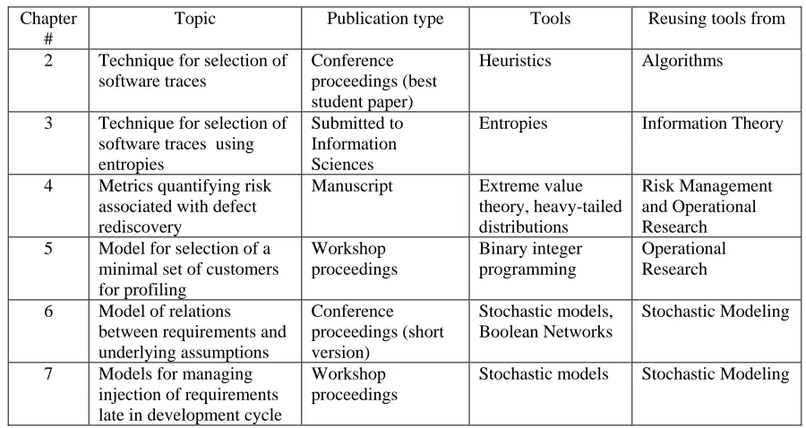
Table 1. Papers: summary information ... 6

Table 2. Applicability of the papers to software development phases (X marks applicable area)... 6

Table 3. Descriptive statistics of traces... 36

Table 4. Dictionaries of a trace given in Figure 11... 51

Table 5. Example: Relation between traces and defects... 56

Table 6. Example: Traces sorted by distance and ranked... 57

Table 7. Example: Top 1-4 defects ... 57

Table 8. Descriptive statistics of length of traces ... 60

Table 9. Fraction of correctly classified traces in Top X for 1) H_E

[

α( ; , );t l c q

]

with ( , , ) E∈ L R T , q∈(10 ,10 )−5 −4 , l= 3, and c=FDT, and 2) set of entropies Λ; based on 10-fold cross validation. Average fraction of correctly classified traces in 10 folds is denoted by “Avg.”; plus-minus 95% confidence interval denoted by “95% CI”. ... 65

Table 10. Percent of correctly classified traces in Top X for H_E

[

α( ; , );t l c q

]

, E=L, = 3 l , and q= {10 ,10 }−4 −5 ... 67

Table 11. AIC... 90

Table 12. Values of variables... 93

Table 13. Results of the G/M/k model for v.4, second year. ... 102

(15)

xiv

Table 15: Example. Defects’ discovery ... 113

Table 16. Percentage of the total number of customers needed to cover X% of defects discovered at least Y times ... 117

Table 17. Example 4.1. State changes of assumptions. ... 132

Table 18. Assumptions properties... 142

Table 19. Requirements properties ... 142

Table 20. Metrics values at T_f = 1 (± denotes standard deviation) ... 145

Table 21. Setup parameters... 155

(16)

xv

List of Figures

Figure 1. An example of a trace... 11

Figure 2. Algorithm for comparing two processes ... 21

Figure 3. Comparison of two uncompressed processes. Upper dashes depict functionality present only in Process 1; lower dashes – functionality present only in Process 2; no dashes – common functionality. ... 22

Figure 4. Algorithm for measuring distance between traces. ... 25

Figure 5. Algorithm for comparing a single trace t against a set of traces S. ... 27

Figure 6. Algorithm for comparing traces within a given set S... 31

Figure 7. Timing of comparing a trace against a set of traces; timing for each draw is denoted by circles; values are plotted on the left axis. Solid line shows the number of comparisons in the lower pattern; dotted line in the upper pattern; values of both lines are plotted on the right vertical axis... 38

Figure 8. Timing of comparing traces within a given set ... 39

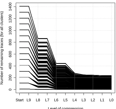
Figure 9. Number of traces remaining after each iteration of comparing traces within a given set ... 39

Figure 10. Predicted time (dotted lines represent 95% confidence bands) for (a) P1(t,S) − linear, and (b) P2(S) − quadratic, based on extrapolation of the fitted regression. ... 41

Figure 11. An example of a trace... 46

Figure 12. Distribution of the number of traces per defect (version) ... 60

(17)

xvi

Figure 14. Interpolated average fractions of correctly classified traces in Top 5 (based on

10-fold cross validation) for E=L and c=FDT. for different values of l and q. ... 63

Figure 15. Fraction of correctly classified traces in Top 5 for E=L, l= 3, q= 10−5, and = c FDT. Solid line shows the average fraction of correctly classified traces in 10 folds; dotted line shows pointwise 95% confidence interval (95% CI) of the average. ... 64

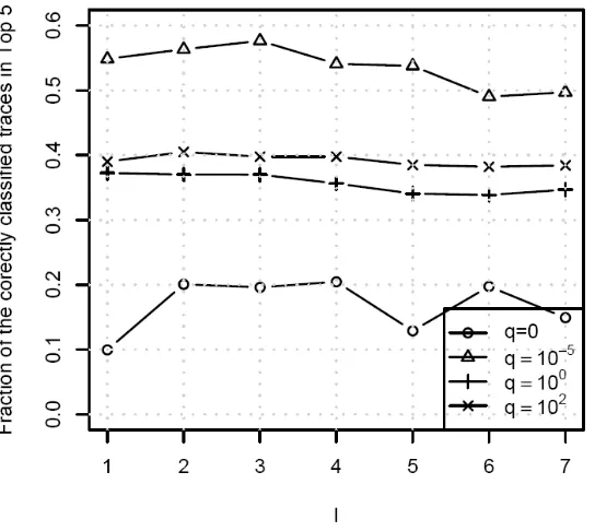
Figure 16. Average fraction of correctly classified traces in Top 5 for various values of l; = E L, q∈(0,10 ,10 ,10 )−5 0 2 , c= FDT... 66

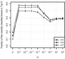
Figure 17. Average fraction of correctly classified traces in Top 5 for various values of q; =E L, (1,3, 7)l∈ , c = FDT ... 68

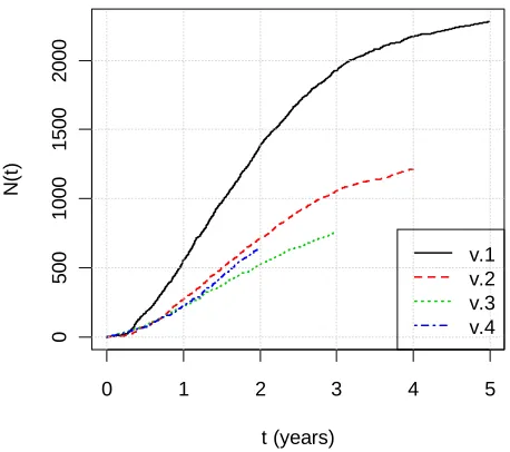
Figure 18. N(t): total number of defects discovered up to time t... 87

Figure 19. R(0,t): total number of rediscoveries up to time t... 88

Figure 20. L-moments ratio diagram of Di for all releases per year (years 1 – 5). The hollow circles denote each of the yearly datasets of Di. The diagram shows the fits of the following distributions: Exponential (EXP), Normal (NOR), Gamma (GUM), Rayleigh (RAY), Uniform (UNI), Generalized Extreme Value (GEV), Generalized Logistic (GLO), Generalized Normal (GNO), Generalized Pareto (GPA), generalization of the Power Law, Pearson Type III (PE3), and Kappa (KAP). Kappa distribution applicability space is a plane bounded by GLO distribution line above and the “Theoretical limits” line below and is not shown on the legend. Based on this figure, Kappa distirbution is the only one that is applicable to modeling each of the datasets. ... 90

Figure 21. QQ plot of the empirical vs. PE3 distributions’ quantiles... 91

Figure 22. QQ plot of the empirical vs. KAP distributions’ quantiles. ... 91

(18)

xvii

Figure 24. Plot of the empirical cdf vs. Compound Kappa distribution theoretic cdf... 95

Figure 25. M1: expected number of defects rediscovered more than d times during the 2nd

year after GA date... 96

Figure 26. M3: expected total number of rediscoveries for defects with number of

rediscoveries above d during the 2nd year after GA date. ... 98

Figure 27. M5: probability that the total number of rediscoveries will not exceed L during

the 2nd year after GA date. ... 99

Figure 28. Estimate that the total number of rediscoveries will not exceed M6with

confidence level α... 100

Figure 29. Density of requests inter-arrival times for v.4, second year... 101

Figure 30. Total number of discovered defects vs. average number of rediscoveries per customer. Dotted lines depict borders of quadrants described in Table 14. ... 115

Figure 31. Percentage of the total number of customers needed to cover a certain

percentage of defects of interest. ... 116

Figure 32. Percentage of the total number of customers needed to cover a certain

percentage of defects of interest (log-scale). ... 117

Figure 33. Example 4.1. Set up of assumptions for a. Configuration I; b. Configuration II. Solid arrows denote standard relationship, dotted arrows denote key relationship... 131

Figure 34. Example 4.2. Five random realizations of ( , )I r t ... 134

Figure 35. Simulation setup. Circles denote assumptions, squares denote requirements. Solid arrows denote standard relationship, dotted arrows denote key relationship... 141

(19)

xviii

Figure 37. The value of ˆ ( , )C ⋅t ... 144

Figure 38. The value of ˆ ( , )U ⋅t ... 144

Figure 39. The value of ˆ( , )I ⋅t ... 145

Figure 40. Dependencies among requirements... 155

Figure 41. Case 1. Expected priority ... 156

Figure 42. Case 2. Expected priority ... 157

(20)

Chapter 1

1 Introduction

In this section, we give a brief exposition to the field of software engineering and the challenges faced in the field. The term “Software Engineering”, and the engineering subfield it describes, was coined in 1968 at the NATO Software Engineering Conference [1]. The IEEE Computer Society Software Engineering Body of Knowledge defines software engineering as:

“(1) The application of a systematic, disciplined, quantifiable approach to the development, operation, and maintenance of software; that is, the application of engineering to software. (2) The study of approaches as in (1)” [2].

This discipline was created to address the “software crisis” increasingly apparent [1], [3] at the time. This crisis described the difficulty of writing correct and maintainable programs as computational power and the concomitant complexity of problems that can be tackled increased. The crisis manifested itself both in: (i) unmanageable projects

running over budget and late1 and (ii) low quality, inefficient software not meeting original requirements. In some cases projects failed completely, being unable to deliver a final product. In order to tackle these issues, well defined and structured approaches had to be developed.

The complexity problem and the need for defined processes can be described using analogies from building construction. While most people can hammer a nail into a wood board, a much smaller fraction of the population (your humble author excluded) is capable of building a doghouse with an even smaller number of people being capable of building a wooden cabin. Increase in the size and complexity of a project demands not

1

(21)

only increased craft skills but also the ability to plan, design, build and test the final product.

Similar to other engineering disciplines, software engineering is divided into a number of knowledge areas [2], [5]. We now describe a few such areas relevant to this thesis. The first four areas can be mapped to specific development phases:

1. Software requirements: deals with elicitation, analysis, specification, and validation of requirements for a given software project.

2. Software design: generates high-level designs (also called architecture) depicting the components and their interfaces, based on specifications elicited during the software requirements phase. Once the high-level design is complete, low-level design of specific components can be created.

3. Software construction: relates to the actual implementation (coding and unit testing) of the product based on design specifications.

4. Software testing: verifies that the implementation satisfies the specifications and is free of defects. Once the testing is complete, the product is deployed in the field.

In practice, the development is done using an iterative and incremental approach [6]: an organization will pass through multiple iterations of requirements, design, construction, and testing between the initial planning and final deployment of the software product.

(22)

The previous five knowledge areas map to specific phases of software development. The remaining two are more general.

6. Software engineering management: relates to project management (and measurement) of software engineering.

7. Software quality control: corresponds to the qualities of the intended system (e.g., reliability of the system, performance, usability, interoperability, portability, maintainability, and others). This area is tightly related to all of the areas listed above.

A significant amount of work has been done improving the software development process and integrating these changes into the industry. However, an analysis (based on literature and empirical evidence) published in 2003 concludes:

“In a discussion of software engineering and society in 1968 [1], Kolence suggests that ‘the basic problem is that certain classes of systems are placing demands on us which are beyond our capabilities and our theories and methods of design and production at this time.’ Empirical evidence of software engineering projects suggests this crucial issue remains valid 35 years after it was stated. It appears that as fast as software engineering makes progress, so the demands made on it continue to increase beyond its capabilities” [7].

(23)

The SEI conducts regular surveys to determine the maturity distribution of processes in the industry. Based on the survey of process maturity profiles [9] the number of organizations with chaotic processes or defined reactive processes (CMMI -1 and -2) went down from ≈35% in 2002 to ≈28% in 2010. The number of organizations with proactive processes (CMMI-3) went up from ≈33% in 2002 to ≈55% in 2010. However,

the number of organizations with highest levels of process maturity (CMMI -4 and -5) focusing on well established, measured and controlled processes and with continuous process improvement went down from ≈23% to ≈10%.

Why is the chaos in Software Engineering higher than in other engineering disciplines [10]? Why is the fraction of organizations with highest process maturity decreasing [9]? Increasing complexity is one of the major contributing factors to the problem [7]. However, there exist additional economic and legal reasons.

The problem is two-fold:

1. Many of the techniques created to improve software processes are non-scalable

[11] – as projects get larger time and resource constraints force some processes2 to be sacrificed at least part of the time.

2. Even if a technique is applicable to a given project, it may not be enforced by the organization due to corporate culture [10]: employees’ performance evaluation may not take into account the use of proper processes.

Potential solutions to this problem are complicated by the fact that the majority of software products (unlike products created using other engineering disciplines) include “as-is” clauses in their licenses stating that a given software vendor does not provide any warranty and shall not be deemed liable for any damage caused by its software products.

2

(24)

This can lead to the situation where the final quality of the product is considered non-critical by some developers. This decreases the economic incentive for software developers to properly engineer solutions.

How should the situation be improved? The first aspect of the problem can be solved by developing fast and scalable solutions supported by proper empirical studies [13], [14]. The second aspect does not have a straightforward solution: it is extremely difficult to change corporate culture [15]. In order to address this issue, newly developed techniques and processes should be capable of being integrated into existing processes without draining significant resources. Namely, they should satisfy the following requirements: a) be easy to implement and b) be easy to automate. Once implemented, a process should run automatically and deliver regular reports in a comprehensible format.

This thesis describes a set of models, techniques, and metrics (satisfying the above mentioned requirements) that can help in the analysis of computer software during various phases of software development.

1.1 Outline

(25)

Table 1. Papers: summary information

Chapter #

Topic Publication type Tools Reusing tools from 2 Technique for selection of

software traces

Conference proceedings (best student paper)

Heuristics Algorithms

3 Technique for selection of software traces using entropies

Submitted to Information Sciences

Entropies Information Theory

4 Metrics quantifying risk associated with defect rediscovery

Manuscript Extreme value theory, heavy-tailed distributions

Risk Management and Operational Research 5 Model for selection of a

minimal set of customers for profiling Workshop proceedings Binary integer programming Operational Research 6 Model of relations

between requirements and underlying assumptions Conference proceedings (short version) Stochastic models, Boolean Networks Stochastic Modeling

7 Models for managing injection of requirements late in development cycle

Workshop proceedings

Stochastic models Stochastic Modeling

Table 2. Applicability of the papers to software development phases (X marks

applicable area)

Development Phases Overall product quality Project management Chapter # Requir-ements Archi- tecture

Coding Testing Mainte-nance

2 X X

3 X X

4 X X X

5 X X X

6 X 7 X

(26)

the role of fingerprints. The techniques in these two papers can accelerate problem determination of defects discovered by customers, leading to improved organizational response (thus increasing customer satisfaction) and to easing of resource constraints.

The third and fourth papers, presented in Chapters 4 and 5, help in addressing issues related to software maintenance and overall quality. Techniques presented in these papers also help project managers in resource allocation.

The third paper analyzes rediscovery of defects by customers and establishes a set of metrics (based on risk management and operational research apparatus) needed to quantify the risks associated with defect rediscovery. The metrics are designed to help: the QA team to assess their processes, the support and maintenance teams to allocate their resources, and the customers to assess the risk associated with the use of the software product.

Collecting information about product usage by customers (operation profiling) helps testers to build realistic workloads, covering functionality executed by customers, hence reducing risks associated with inadequate product quality. However, it is impossible to gather such information from all customers due to resource and legal constraints. The fourth paper establishes a relation between defects encountered by customers and their operational profiles. We then build a model for selecting a minimal set of customers that should be profiled to gather information about users’ behaviour.

The fifth and sixth papers deal with problems from the domain of requirements engineering.

(27)

The sixth paper, presented in Chapter 7, defines stochastic models for managing risk associated with requirements injected late in the software development cycle (we call this event escalation). The models can help in predicting escalations of the existing requirements and in allocating resources to handle the arrival of unknown requirements. Finally, Chapter 8 concludes the thesis.

References

[1] P. Naur and B. Randell, “Software Engineering: Report of a conference sponsored by the NATO Science Committee Garmisch Germany 7th-11th October 1968,” Scientific Affairs Division, NATO, 01-Jan-1969.

[2] A. Abran, P. Bourque, R. Dupuis, J. Moore, and L. Tripp, Guide to the Software Engineering Body of Knowledge - SWEBOK. IEEE Press, 2004.

[3] E. W. Dijkstra, “The humble programmer,” Commun. ACM, vol. 15, pp. 859–866, Oct. 1972.

[4] E. Yourdon, Death March, 2nd ed. Prentice Hall, 2004.

[5] “Industry implementation of International Standard ISO/IEC 12207: 1995. (ISO/IEC 12207) standard for information technology - software life cycle processes - life cycle data,” IEEE/EIA 12207.1-1997, 1998.

[6] C. Larman and V. R. Basili, “Iterative and incremental developments. a brief history,” Computer, vol. 36, no. 6, pp. 47 - 56, Jun. 2003.

[7] C. L. Simons, I. C. Parmee, and P. D. Coward, “35 years on: to what extent has software engineering design achieved its goals?,” Software, IEE Proceedings -, vol. 150, no. 6, pp. 337 - 350, Dec. 2003.

[8] CMMI Product Team, CMMI for Development, Version 1.3; CMU/SEI-2010-TR-033. Software Engineering Institute of Carnegie Mellon University, 2010.

[9] CMMI Appraisal Program Team, “Process Maturity Profile. CMMI For

Development SCAMPI Class A Appraisal Results 2010 Mid-Year Update,” Sep-2010.

[10] D. L. Parnas, “Risks of undisciplined development,” Commun. ACM, vol. 53, pp. 25–27, Oct. 2010.

[11] A. V. Miranskyy et al., “SIFT: a scalable iterative-unfolding technique for

filtering execution traces,” in Proceedings of the 2008 conference of the center for advanced studies on collaborative research: meeting of minds, pp. 274-288, 2008.

(28)

[13] E. J. Weyuker, “Software engineering research: from cradle to grave,” in Proceedings of the the 6th joint meeting of the European software engineering conference and the ACM SIGSOFT symposium on the foundations of software engineering, pp. 305–311, 2007.

[14] P. Runeson and M. Höst, “Guidelines for conducting and reporting case study research in software engineering,” Empirical Softw. Engg., vol. 14, pp. 131–164, Apr. 2009.

(29)

Chapter 2

2 SIFT: A Scalable Iterative-Unfolding Technique for

Filtering Execution Traces

Comparing program execution traces can be useful for numerous purposes, such as software testing, system security analysis, program comprehension, software evolution and other areas of software development. Unfortunately, trace comparison techniques that operate on execution traces containing full execution details are too slow for use in large-scale production system environments. In order to speed up the comparisons, we propose a technique (called SIFT) for "filtering-out" irrelevant traces from a given set so that only the relevant few residual traces are then used for comparison. Our solution involves multiple levels of trace compression, each with a different degree of abstraction. These traces are compared iteratively while filtering out dissimilar traces. This chapter describes the compression and comparison algorithms. Prototype results from a significant case study show that the SIFT approach is efficient and scalable for use in an industrial software development environment.

2.1 Introduction

(30)

For some problems, such as test case prioritization, traces gathered in a condensed form (such as a vector of executed function names or caller-callee pairs) are adequate [8]. However, for others, such as the detection of missing coverage and anomalous behaviour using state machines, detailed execution paths are necessary [4, 21]. Also, in some situations, the time required for analysing traces can be extremely important, for example when a customer support analyst is using traces to map a reported defect onto an existing set of defects, or when a development analyst is working with the testing team to identify missing coverage that resulted in a field defect.

In general, a trace can be thought of as a sequential log of pertinent information

captured during any particular execution-run of software. This trace shows program flow

entering functions3 f1, f2, and f3, and eventually exiting these functions and, while in

function f3, it reached specific data points (probe 1 and probe 2), which were manually

set by the developer as points of interest.

Figure 1. An example of a trace

Research Problem and Practical Motivation: Unfortunately, comparison techniques that

use full execution paths (i.e., do not use some abstracted versions of the paths) lack speed, which can become critical when using numerous large execution traces. For

3

In this case a function is equivalent to a subroutine.

process_id = 133 thread_id = 15 node = 0 1 f1 entry

2 | f2 entry 3 | | f3 entry

(31)

example, the kTail-based algorithms4 applied to traces from a reference system, called Object Flattener, (for the purpose of creating finite state automata – which would involve comparing given traces) did not terminate after 24 hours of execution [4]. While the kBehavior algorithm [4] accomplished this task in “minutes”, their paper does not mention the size or the number of traces involved in Object Flattener. Subsequently, we applied kBehavior prototype tool [15] on traces from our environment. With only 2 traces totalling 426 elements (the smallest in our set of traces), the tool took 9 minutes; with 36 traces totalling 8625 elements (considered small in our environment), it did not terminate after 36 hours. Finally, various permutations of up to 57 traces and up to 68,705 elements consistently caused the kBehavior prototype to crash. These experiences highlight the need for speed and robustness of the solutions.

In our development environment, we are faced with a distributed, multi-process, and multi-threaded system of over 10 million lines of uncommented source code developed over 15 years, with over 100 thousand traces (many with millions of elements per trace) from the testing phase. There are hundreds of thousands of installations worldwide of the system, in different configurations. As a result, a critical issue surfaced as to how quickly the testing organization could identify those test cases that match the traces collected from the field upon recognition of a defect or a problem such as a logic error. While there are many different approaches to performing trace comparisons, they are not considered workable, as described earlier, for the large and complex system we are dealing with. The described need to match field traces with test cases quickly, together with a lack of reliable and scalable tools for doing this, motivated us to investigate alternate solutions.

Solution Approach: To speed up comparison of traces, we propose that traces first be

filtered out from the given set, rejecting those that are not going to match with the test cases and then only the remaining few be compared for target purposes. The underlying

4

(32)

assumption is that most traces in a given set will not be the same; few will be similar, and even fewer will be identical. We validated this assumption in our sample set of traces by manual inspection of the dataset. Thus, filtering out irrelevant traces is a key to speeding up the comparison process.

This strategy is implemented in our solution called the Scalable Iterative-unFolding Technique (SIFT). Basically, the collected traces are first compressed into several levels prior to comparing them. Each level of compression uses a unique signature, which we

call a “fingerprint”5. Then, starting with the highest level of compression the traces are compared, and unmatched ones rejected, while iterating through the lower levels until the comparison process is complete, leaving only traces that match at the lowest (or uncompressed) level. The SIFT objective ends here. The matched traces can then be passed on to external tools for further analysis such as code coverage, security breaches, and operational profiling.

Case study: The prototype results from a case study we conducted show that the approach

is scalable for use in large-scale software system development environments. That is, in no more than four iterations (depending on the context of the specific problem being solved), dissimilar traces are rejected, leaving only the residual similar traces. The case study was conducted on 1416 multithreaded test case traces collected from the system under study (SUS), with an average length of 1.93×106_{elements (maximum 1.55×10}8

elements) per trace. The first test was comparing a trace against a set of 1,000 traces (e.g., useful for coverage analysis); the average time was 4 seconds. The second test was “within-set” filtering and clustering (e.g., useful for periodic profiling of usage similarity among a class of users or a class of test cases); the average of comparing multiple times within a set of 1,000 traces was only 44 minutes.

5

(33)

Based on the extrapolation of the timing data obtained from the case study, it should take 39 seconds on average to filter out 10,000 different traces, leaving, as a residue, a few uncompressed traces that are within the user-defined threshold of similarity. Similarly, filtering (and clustering) within a set of 10,000 traces should take 2.6 days on average. We consider the “within-set” performance as quite reasonable, and encouraging, given that such profiling would occur only periodically in a product’s life. Considering the lack of readily available solutions for use in industrial-scale environments, the proposed approach is both elegant and effective.

The rest of the paper is structured as follows: Section 2.2 reviews related literature. Section 2.3 details the SIFT and associated algorithms. Section 2.4 analyses the efficiency and accuracy of the SIFT. Section 2.5 describes an implementation and use of the proposed approach. Section 2.6 describes the case study. Finally, Section 2.7 gives conclusions and describes future work.

2.2 Related Work

A variety of different approaches (such as, automata, signals, call-graphs, compression without information loss, and clustering) exist in dealing with execution traces for various target purposes such as finite automata representation, visualization, test-case prioritisation, and failure classification. These are overviewed below.

Finite State Automata representation: There is a family of kTail-based algorithms that

(34)

are merged if a k-feature of the first state is included in the k-feature of the second state). All of the algorithms above need to process all traces first before generation of the interaction model can begin. Mariani and Pezze [21] developed an algorithm, called kBehavior, that overcomes this issue and works incrementally. These techniques may be used to determine how well user execution paths (traces collected in the field) are covered in testing [4], detecting anomalous behaviour arising during a component’s upgrade or reuse [21], and general program comprehension [28].

Signal representation: Kuhn and Greevy [16] visualize multiple execution traces in signal

form, discarding information about function names. Once conversion to signal form is complete, a Dynamic Time Warping (DTW) pattern recognition technique is used to find similar patterns between traces. This approach is used to compare detailed execution traces for program comprehension. Unfortunately, patterns of execution paths containing different function calls may have similar shapes. This is especially true for large software systems consisting of multiple processes. Therefore, it is important to group (pre-filter) the traces containing similar execution paths, before conversion to the signal form. Once pre-filtering is complete, an analyst can apply the DTW technique to each of the groups separately.

Call graph representation: Another approach patented by Avvari et al. [1] is the idea of

creating and analysing call graphs. Execution paths (EP) are first converted into call graphs and then compared in graph form. In practice, the quantity and complexity of EP in a large software system would not allow one to perform this comparison directly in a feasible amount of time. For example, for a large software system, the number of test cases can be of order of 105, with the number of records per EP of the order of 106. The performance of the publicized algorithms is, at best, of ⎡ _{V E}_log

(

_V2_/_E

)

_{/ log}( )_V ⎤

⎢ ⎥

⎣ ⎦

O , where V is

(35)

Lossless compression techniques: With these techniques, it is possible to reconstruct the

exact original data from the compressed data. Renieries et al. [29] introduce lossless compression techniques for source-code-level traces that lead to significant compression of the original traces. Techniques, such as that designed by Hamou-Lhadj and Lethbridge [12] can be used for visualizing traces in a compact form, which can be useful for viewing several traces on a display screen during software maintenance.

Lossy compression techniques: With these techniques, reconstruction of the exact original

data from the compressed data is not possible. There are both short and long execution sequences, used for various purposes. In the realm of short sequences, for example, Elbaum et al. [8] found that function-name-level execution traces can be useful for test case prioritization. Rothermel et al. [30] and Masri [22] used the same type of traces to perform test suite reduction/minimization by identifying redundant traces. Greevy et al. [11] explore relations between features (function names) extracted from traces and software entities for software evolution analysis. Yuan et al. [31] found that for system call defects, caller-callee-pairs-level execution traces (with parameter information) were effective for mapping a new problem to an existing one. In the realm of long sequences, for example, Miranskyy et al. [23] show that sequences of length 3 or more are potentially important for test case prioritization. Elbaum et al. [7] found that sequences of length 5 are useful for fault detection. Dalmeier et al. [5] studied sequences of various lengths (no more than 8) to localize defects. Lee et al. [17] found execution sequences of length 7 and 11 to be useful for intrusion detection.

Trace clustering techniques: In addition, researchers have created techniques to compare

(36)

address the challenge of comparing detailed uncompressed traces so the need to filter the traces remains.

While there are many techniques, as described above, researchers have not considered the idea of filtering-out traces to improve comparison of uncompressed traces. This is the bounded scope that is addressed by our work described in the next section.

2.3 Method Description

In this section, we first describe the basics of the SIFT approach in Section 2.3.1. As overviewed in the introduction section, this approach filters out traces from a given set that are not going to match with the test cases, leaving a few for detailed comparison. Section 2.3.2 then describes the algorithms underlying this approach. The analysis of these algorithms is carried out in Section 2.4.

2.3.1 The Iterative-Unfolding Approach

Further to the introductory description earlier, the idea behind the SIFT approach is two-fold.

Unfolding: First, traces to be compared can exist at different levels of compression. For

example, at the lowest level of compression, a trace would be at the level of detail captured from program execution, where a sequence of function calls is represented as a string of calls. A slightly higher level of compression could be, for example, where this string of functions calls is broken down into “caller-callee” pairs. A yet higher level of compression could be just a list of function names. The type of compression applied and the number of compression levels is analyst defined and should be selected in such a way that the current iteration compression technique retains less information than the next iteration.

(37)

directly to the program-level (or lowest-level) trace. Compression techniques and compression levels are independent of each other. Note that any compression technique can be used for trace compaction, as long as a certain measure of distance can be calculated between a pair of compressed traces.

The full scope of the type of data involved in a trace can include a wide variety of program elements such as: events, logic-based points in the program flow, store & retrieve transaction points, and process enaction or termination points. We define a process as an instance of a sequentially executed computer program.

Iterative: The second idea behind the SIFT approach is that it proceeds by comparing

stored traces at the highest level of compression and, based on the outcome of this comparison (that is, a set of matched and unmatched traces), discards the unmatched set of traces and proceeds to compare the matched set of traces at the next lower level of compression until a terminating condition is satisfied. The terminating conditions are: (1) the number of traces remaining for comparison is below a certain threshold; (2) no lower levels of compression of traces exist; and (3) practical conditions such as exhausting time and resources.

A benefit of this approach is that it makes comparison of large program traces or large volumes of traces practical. Later, we discuss the various permutations of trace comparison situations and how our approach fares with these.

2.3.2 Algorithms

(38)

There are several fundamental types of situations for comparing execution traces:

(a) A single trace t against a set of traces6S. We can represent this comparison process by a function P1 that takes as input two variables of interest, trace t and a set of traces S,

and outputs a subset of traces S1 closest

7 to t:

P1(t, S) → S1.

One example of this situation is where the single trace is captured from the system’s use in the field, hereafter called User Trace (UT); by contrast, the set represents the traces captured from the execution of test cases, hereafter called House Traces (HT). This is useful for identifying a subset of HTs that match the given UT for a purpose such as coverage analysis, or for that matter, for identifying mismatches for the purpose of proactively creating new test cases.

(b) Within a given set of traces S. Here, the comparison function P2 clusters S into L subsets of similar traces:

P2(S) → {S1, S2, …, SL}.

One example of this situation is comparing a set of UTs against itself to profile subsets of customers with similar system usage needs. The outputs of the comparison process are subsets of similar and different traces.

In the next section, we describe how the comparison of two given traces is performed.

6

This approach can be further generalized to comparing two sets of traces, see [24] for further details.

7

(39)

2.3.2.1 Core Algorithms: Fingerprints, Processes, and Traces

There are a number of algorithms that are used for the SIFT approach. For the sake of clarity, we will first explain each algorithm and then continue with the description of the overall approach.

First, as described in Section 2.1, there is the notion of a “fingerprint”. The fingerprinting technique is described in Section 2.3.2.1.1. Also, we introduced the notion of a process in Section 2.3.1. Traces contain information about multiple processes executed in parallel (mostly independently). To align execution sequences pairwise comparison of processes has to be implemented. The algorithm for comparing a pair of processes is described in Section 2.3.2.1.2. We then describe the algorithm for comparing a pair of traces, building upon process comparison, in Section 2.3.2.1.3. The overall approach binding fingerprints, processes and traces is described in Section 2.3.2.1.4.

2.3.2.1.1 Fingerprints

A “fingerprint” of a process describes the uniqueness of the process in terms of the call sequence, elements of contextual information, and other relevant information that make up the fingerprint. The first technique for creating fingerprints would be the collection of component names along with the frequency of occurrence contained in each process. On average, the number of components per process is of order 101. In most cases, it should not be bigger than 102. Similarly, information about function names can be collected.

In order to collect the next set of fingerprints we use a concept of l-words (also known as N-grams [31]) to represent execution sequences. An l-word represents a continuous substring of length l from a string. We then collect information about all possible entry, exit, and probe points (defined manually by software developers at important places inside the functions) and their frequency for each process (1-words) and end up with all possible pairs of entry, exit, and probe points (2-words). For example, for the process given in Figure 1, the set of all possible 1-words will be given by the set

{

1 2

}

1 , 2 , 3 , 3, 3 , 1 , 2 , 3 ,

(40)

name index and the upper index k represents the record type: + for an entry, − for an exit,

and number for a probe point k. 2-words will be represented accordingly by the set

{

1 1 2 2

}

1 2 , 2 3 , 3 3, 3 3 , 3 3 , 2 1 , 3 2 .

f f+ + f f+ + f f+ f f f f− f f− − f f− − All 1- and 2- words are unique in this

case – their frequencies are equal to 1.

Additional measures, such as Entropy measures [6] or N-stacks , can be introduced as needed. If a user is interested in calculating exact matching between traces, then hashing techniques can be used for compression. However, these techniques are not applicable for approximate trace matching, since no non-trivial measure of distance can be established between hashed traces.

2.3.2.1.2 Algorithm for Comparing a Pair of Processes

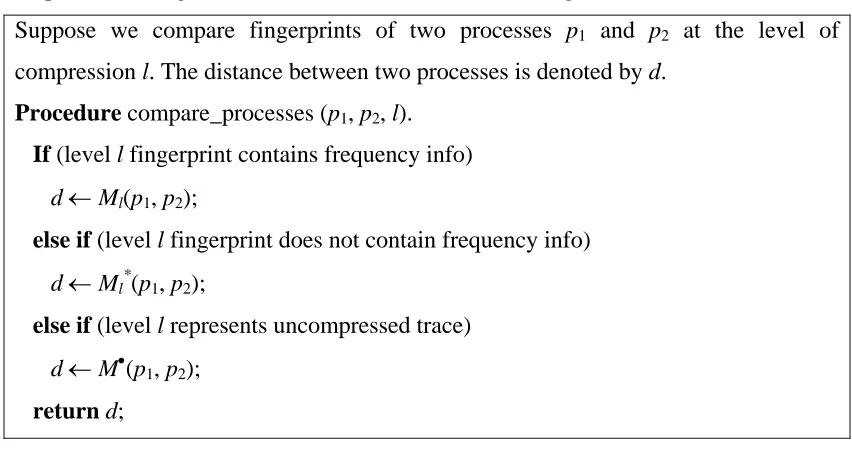
We summarize the algorithm for comparing a pair of processes at different levels of compression in Figure 2. Functional forms of Mk(X,Y) are given below.

Suppose we compare fingerprints of two processes p1 and p2 at the level of

compression l. The distance between two processes is denoted by d. Procedure compare_processes (p1, p2, l).

If (level l fingerprint contains frequency info)

d ← Ml(p1, p2);

else if (level l fingerprint does not contain frequency info)

d ← Ml*(p1, p2);

else if (level l represents uncompressed trace)

d ← M•(p1, p2);

return d;

Figure 2. Algorithm for comparing two processes

(41)

distance between two uncompressed traces we use the Levenshtein distance8 [18], denoted by MU. An example of comparing two processes is given in Figure 3.

For comparing two compressed processes X and Y at the level of compression k (see Section 2.3.2.2 for details), we use the following metric:

[ ( ), ( )], if

( , ) ,

, if

X Y i k

X i Y i X Y

M X Y

X Y λ ∪ ⎧ _∑ _{∩ ≠ ∅} ⎪ = ⎨ ⎪∞ ∩ = ∅ ⎩ (2.1)

where

(

)

(

)

max , 1

( , ) 1,

min , 1

α β λ α β

α β +

= −

+ and X(i) and Y(i) will return the value of the i-th

member in the set, e.g., frequency of occurrence, or zero if the member is absent. The summation is performed for all elements of sets X and Y (X ∪ Y). We add 1 to both the

numerator and the denominator to avoid division by zero and subtract one from the ratio to get 0 if X(i) = Y(i).

1 1 1 3 3 3 1

2

2 1 2 3 3 3 2 1

1 2

1 2 1 2 3 3 3 3 2 1

, ,

.

p f f f f f

p f f f f f f f

p p f f f f f f f f

+ + − − + + + − − − −− −− −− + + + − − − −− = = ↔ =

Figure 3. Comparison of two uncompressed processes. Upper dashes depict

functionality present only in Process 1; lower dashes – functionality present only in

Process 2; no dashes – common functionality.

Note that the usage of p-norms, e.g., Euclidean norm is not desirable; since they will not highlight information about non-overlapping set members, while metric (2.1) will; see Example 1 for details.

8

(42)

Example 1.

Suppose we have two processes: A containing components a and b with frequencies 4 and 3 accordingly; B containing components a, b, and c with frequencies 5, 3 and 1; and C containing components a, b, and c with frequencies 4, 3 and 2. We can write these fingerprints as three vectors: A = [4 3 0], B = [5 3 1], and C=[4 3 2].

By calculating the distance between processes9 (

2

A B− denotes Euclidiean distance between A and B) we get

2

( , ) [0.2 0 1] 1.2,

( , ) [0 0 1] 1.0,

|| || [1 0 1] 2.0,

|| || [1 0 1] 2.0.

M A B

M B C

A B B C = = = = − = = − = =

∑

(2.2)

Euclidean norm treats all dimensions equally; it shows that the distance between processes A and B is the same as between processes B and C. However, we want to emphasize the fact that A and B are further apart than B and C, since component c is missing in A and metric M highlights this fact.

For those fingerprints that do not contain frequency information (vectors whose i-th value is 1 when the element is present in the uncompressed trace and 0 otherwise), we can use a simple metric * 0, ( , ) . , k X Y

M X Y

X Y

∩ ≠ ∅ ⎧

= ⎨_∞ _{∩ = ∅}

⎩ (2.3)

This measure is conservative, but is rather fast to compute

9

(43)

2.3.2.1.3 Algorithm for Comparing a Pair of Traces

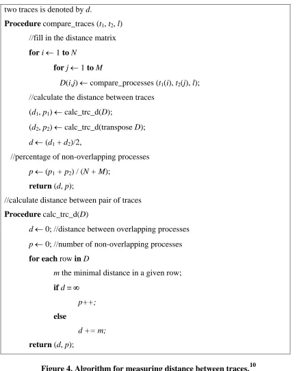
Since the traces consist of multiple processes, we need to perform cross-comparisons between each pair of processes and aggregate this data to obtain a quantitative description of the distance between traces. To do this, we need a (possibly heuristic) distance measure that calculates the distance between a pair of similar traces to be less than the distance between a pair of less similar traces.

No simple one-dimensional measure of a complicated concept such as the “difference between two traces” can capture all desired features. Is Moby Dick closer to the Book of Genesis than it is to the Catcher in the Rye? It is unlikely that a simple heuristic can be devised that answers this question to everyone’s satisfaction. Nevertheless, we need a heuristic. Our heuristic is defined in Figure 4.

2.3.2.1.4 The Overall Approach

The algorithms implement SIFT through trace and process comparison, as well as fingerprinting. During software execution, in a concurrent processing environment, a trace t could consist of the multiple, parallel, processes executed during the software run. If the total number of processes in a given trace t is equal to m then

t = {p1, p2, …, pm}.

Later, we will use this information to compute the similarity between given traces. In general, a process may split into multiple threads. For the sake of simplicity, in this paper we assume that each process consists of a single thread – henceforth processes and threads are treated as equal. Comparing two multi-threaded processes is analogous to comparing two traces with multiple processes.

Suppose we compare two traces t1 and t2 with number of processes equal to N and M

respectively at the level of compression l. Distances between processes of t1 and t2

(44)

two traces is denoted by d.

Procedure compare_traces (t1, t2, l)

//fill in the distance matrix for i ← 1 to N

for j ← 1 to M

D(i,j) ← compare_processes (t1(i), t2(j), l);

//calculate the distance between traces

(d1, p1) ← calc_trc_d(D);

(d2, p2) ← calc_trc_d(transpose D);

d ← (d1 + d2)/2,

//percentage of non-overlapping processes

p ← (p1 + p2) / (N + M);

return (d, p);

//calculate distance between pair of traces Procedure calc_trc_d(D)

d ← 0; //distance between overlapping processes p ← 0; //number of non-overlapping processes

for each row in D

m the minimal distance in a given row;

if d = ∞

p++;

else

d += m;

return (d, p);

Figure 4. Algorithm for measuring distance between traces.10

10

(45)

Let the set of all possible elements of contextual information that can be captured during software execution be denoted by E. A process p with n elements is represented by a sequence

1 N i i

p=e ₌ (2.4)

where i indexes the ith event captured, and each event e∈E. In order to compute the distance between two given traces, we need to compute that measure in terms of the distance between the respective sets of processes contained within the two traces. In essence, we perform cross-comparison between each pair of processes (one process from each of the two given traces) to obtain their distance, and aggregate this data to obtain a quantitative measure of the distance between the two given traces. The distance between two given processes is computed as follows:

compare_processes(prc_id1, prc_id2, c_l) → d_p

where, prc_id1 and prc_id2 are processes at the level of compression c_l; and the comparison process returns a measure of distance between processes d_p. Compare_processes is outlined in Section 2.3.2.1.2.

The process information can be compressed (using lossy compression techniques, i.e., compression with loss of information) into the “fingerprints” introduced in Section 2.3.2.1.1. Individual uncompressed processes are independently compressed, using different compression formulae, to obtain various compression levels. The level of compression of a process specifies the type of fingerprint that should be used in the comparison procedure.

Based on process comparison, we can now describe how the traces are compared. The comparison procedure within any given context considered in Section 2.3.2.1 is defined as follows:

(46)

where trc_id1 and trc_id2 are execution traces at the level of compression c_l; and the output of this comparison is given by a tuple of distance measure between traces d_t and percentage of non-overlapping processes p_p. The parameter c_l is set by the analyst and is, in fact, passed on to the compare_processes procedure discussed above. Details of compare_traces are given in Section 2.3.2.1.3.

2.3.2.2 The Iterative-Unfolding Algorithms

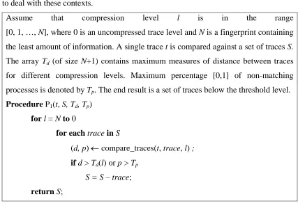
As described in Section 2.3.1, the traces are compared iteratively from the highest to the lowest level of compression. During each iteration, the comparison follows the procedure described in Section 2.3.2.1.4. Recall from Section 2.3.2 that there are two practical contexts for comparing traces: (i) a single trace against a set of traces and (ii) within a given set of traces. Thus, Figure 5 and Figure 6 respectively describe the two algorithms to deal with these contexts.

Assume that compression level l is in the range [0, 1, …, N], where 0 is an uncompressed trace level and N is a fingerprint containing the least amount of information. A single trace t is compared against a set of traces S. The array Td (of size N+1) contains maximum measures of distance between traces for different compression levels. Maximum percentage [0,1] of non-matching processes is denoted by Tp. The end result is a set of traces below the threshold level. Procedure P1(t, S, Td, Tp)

for l = N to 0

for each trace in S

(d, p) ← compare_traces(t, trace, l) ;

if d > Td(l) or p > Tp

S = S – trace;

return S;

(47)

The traces are clustered using the Agglomerative Hierarchical Clustering (AHC) algorithm [14]. It is computed by a function cluster(d_m,d_t),which takes the distance matrix between traces d_m and the maximum distance between traces to be clustered d_t. The distance between clusters is determined by measuring the maximum distance between elements of each cluster. The clustering is stopped when, based on a particular

distance criterion11, the clusters are too far apart to be merged.

2.4 Analysis

In this section we analyze the algorithms presented in Section 2.3.2. The efficiency analysis of the functions is described in Section 2.4.1. Section 2.4.2 describes constraints within which the algorithms are accurate. Section 2.4.3 describes the overhead due to our approach.

2.4.1 Efficiency

In Section 2.4.1.1 we discuss efficiency of the core algorithms. Efficiency of the Iterative-Unfolding Algorithms is shown in Section 2.4.1.2. Special cases are discussed in Section 2.4.1.3.

2.4.1.1 Core Algorithms Efficiency

The derivation of our algorithms asymptotic behaviour may be found in [24]. Only the final results are presented here. Look at the maximum number of algorithm operations required to compare a single trace t against a set of traces S (given in Figure 5). In the worst-case scenario, when all traces within S are close to t and cannot be filtered out, we will have to perform all iterations on the full set |S|:

(

) (

)

2

(

)

0

max 2 2 2 2 2

1 0 0

[ ( , )] | | | | | |

l KL L l

C P t S K S N L S N L S N L

α β

<

∈O +O = O (2.5)

11

(48)

where K is the maximum level of compression, N is the maximum possible number of

processes in a trace and Ll is the maximum length of a given fingerprint at compression

level l. The comparison for l > 0 is performed using measures of distance (2.1) and (2.3); comparison of uncompressed traces is performed at l = 0 (using diff[26]), see Section 2.3.2.1.2 for details. The term α arises from comparison of fingerprints and the term β

from comparison of uncompressed traces. Note that, in practice, most traces will be filtered out at high levels of compression and that the length of fingerprints, by construction, should be small.

The algorithm for comparison within a set of traces calls a recursive procedure “compare” (given in Figure 6). The running time, T, of the function “compare” can be represented as

(

)

1

(| |) | | / compare( ),

a

i S

i

T S T S b

=

∑

⎢_⎣ ⎥_⎦ + P (2.6)

where P_S is a set of properties of traces in set S. Coefficients bi (fraction of elements in S) and a (number of clusters) change at each iteration − they are obtained from the

clustering procedure (called from “compare”) and will depend onP_S.

The problem formulated in (2.6) is too general and, to the best of our knowledge, cannot be “unraveled” without knowing distributions of the parameters bi and a. The worst-case scenario is when a=1 and bi=1, i.e., members of the set S cannot be partitioned into subsets since they are too close to each other. In this case

(

) (

)

2

(

)

0

max 2 2 2 2 2 2 2 2

2 0 0

[ ( )] | | | | | | .

l KL L l

C P S S KN L S N L S N L

<

∈O +O = O (2.7)

In closing, the worst-case scenario computational time for P1(t,S) grows linearly with the

(49)

of traces. The algorithm P2(T,S) is quadratic in the number of traces, the number of

processes per trace and the length of traces.

Assume that compression level l is in the range [0, 1, … , N], where 0 is an uncompressed trace level and N is a fingerprint containing the least amount of information. The initial set of traces is given by trace set S. S(i) returns the i-th member of the set S. Array Td (of size N+1) contains the maximum measures of distance between traces for different compression levels. Maximum percentage [0,1] of non-matching processes is denoted by Tp. Global variable Sout stores similar clusters of traces.

//Transform 2-tuples distance measure into a scalar Procedure condense_tuple(d, p, Tp)

if p > Tp

m ← ∞;

else

m ← d;

return m;

//recursive comparison function (note that recursion can be //“unraveled” by parsing the tree in breadth)

Procedure compare (trace_set, l, Td, Tp)

//calculate distance matrix D between traces M ← cardinality(trace_set);

for i=1 to M

for j=i+1 to M //D is symmetric

(d, p) ← compare_traces(trace_set(i), trace_set(j), l);

D(i, j) ← condense_tuple(d, p, Tp);

//Cluster traces using distance data in D

clusters ← cluster(D, Td(l));

if (l > 0)

(50)

compare(cluster, l − 1, Td, Tp)

else //reached uncompressed level add trace_set to Sout; //main procedure

Procedure P2(S) Set Td and Tp;

compare (S, N, Td, Tp); return Sout ;

Figure 6. Algorithm for comparing traces within a given set S.

2.4.1.2 Special Cases

We identify two cases where the direct comparison approach is more efficient than the iterative-unfolding approach. The first case occurs when the traces of interest are very similar; the traces won’t be filtered out at higher levels of comparison and so direct comparison becomes necessary at the uncompressed level. The second case occurs when the traces are small (i.e., the length of the processes in the traces is comparable to the length of the fingerprints) and the traces consist of only a few processes so comparison times between the iterative-unfolding approach and uncompressed comparisons would be more or less equivalent. Note that if the number of processes is large, our approach may yield superior results by aggregating information from different processes into a single fingerprint. In all other cases, our approach is superior.

(51)

2.4.2 Method Accuracy

In order for the iterative-unfolding approach to be accurate, similar traces must not be accidentally discarded at high levels of compression (we throw away all traces farther apart than a level-specific threshold). To accomplish this, we must carefully select the

threshold’s values for distance measures12 between traces. General guidance is given by the following conjecture (axiomatic in nature).

We conjecture that for every distance threshold Tk+1 > 0 at level k + 1 there exists another threshold Tk > 0 for level k, such that if dk+1(A,B) > Tk+1 then dk(A,B) > Tk. (where dj(A,B) represents the measure of distance between traces A and B at compression level j). This conjecture is reasonable but we have not proved it, nor do we have an explicit way to compute Tk from Tk+1 except in some special cases as detailed below. Traces A and B are considered dissimilar at compression level j if dj(A,B) > Tj. If they are not dissimilar, they are considered to be similar. Our conjecture now states that if two strings are dissimilar at a high level of compression, they will also be dissimilar at the corresponding lower level of compression. For the example of strings with N letters, each taking two values, where lexical distance d0 is between 0 and N and letter count distance d1 is also

between 0 and N, T:=T1= T0. In this case, it follows that if two compressed strings

are dissimilar at level 1 with threshold T, they must also be dissimilar at uncompressed level 0 at the same threshold T.

If this conjecture holds, an analyst can specify the desired zero compression threshold T0

and use the conjecture backwards to generate thresholds for all other levels T1, …, TK, where K is the highest level of compression13.

12

Examples of measures of distance are given in Section 2.3.2.1.2.

13

Models, Techniques, and Metrics for Managing Risk in Software Engineering

Scholarship@Western

Scholarship@Western

Models, Techniques, and Metrics for Managing Risk in Software

Models, Techniques, and Metrics for Managing Risk in Software

Engineering

Engineering

Andriy Miranskyy

Models, Techniques, and Metrics for Managing Risk

in Software Engineering

Abstract

Keywords

Co-Authorship Statement

Acknowledgments

Dictionary and Abbreviations

Table of Contents

List of Tables

[

]

[

]

List of Figures

Chapter 1

1

Introduction

1.1

Outline

References

Chapter 2

2

SIFT: A Scalable Iterative-Unfolding Technique for

Filtering Execution Traces

2.1

Introduction

2.2

Related Work

(

)

2.3

Method Description

2.3.1

The Iterative-Unfolding Approach

2.3.2

Algorithms

2.3.2.1

Core Algorithms: Fingerprints, Processes, and Traces

2.3.2.1.1

Fingerprints

{

}

{

}

2.3.2.1.2

Algorithm for Comparing a Pair of Processes

(

)

(

)

∑

∑

∑

∑

2.3.2.1.3

Algorithm for Comparing a Pair of Traces

2.3.2.1.4

The Overall Approach

2.3.2.2

The Iterative-Unfolding Algorithms

2.4

Analysis

2.4.1

Efficiency

2.4.1.1

Core Algorithms Efficiency

(

) (

)

(

)

(