Modelling hyperfine interactions for nuclear
g
-factor measurements
B. P. McCormick1,∗, A. E. Stuchbery1,∗∗, A. Goasduff2, A. Kusoglu2,3, and G. Georgiev1,2
1Department of Nuclear Physics, Research School of Physics, The Australian National University, ACT 2601, Australia 2CSNSM, CNRS/IN2P3, Université Paris-Sud, UMR8609, F-91405 ORSAY-Campus, France
3Department of Physics, Faculty of Science, Istanbul University, Vezneciler/Fatih, 34134, Istanbul, Turkey
Abstract.A promising technique forg-factor measurements on short-lived nuclear states utilises the hyperfine fields of free ions in vacuum. To fully utilise this technique the hyperfine interaction must be modelled based on atomic structure calculations. Atomic structure calculations were performed using the most recent release of the General Relativistic Atomic Structure Package, and Monte-Carlo simulations of atomic-decay cascades in highly charged ions were developed. The simulations were used to fit experimental data on excited56Fe ions recoiling in vacuum with a view to determining the first-excited stategfactor,g(2+1), of56Fe.
1 Introduction
A powerful probe for nuclear structure study is the magnetic dipole moment, µ. Usually, for excited states, the g factor is the quantity measured, where g=µ/I, I being the spin of the state. Thegfactor provides a way to probe the wavefunction of a single state. It is sensitive to the composition of broken proton vs neutron pairs, and the angular momentum they carry. Often, these states have lifetimes in the picosecond range, requiring kilotesla-strength fields to perform g-factor measurements. Such fields can only result from hyperfine interactions. Two useful hyperfine fields are the transient field [1], resulting from the interaction between a ferromagnetic solid and a swift ion traversing it, and the hyperfine field produced by the electron cloud surrounding the nucleus of a free ion [2]. In the late 1960s, Goldringet al. characterised the hyperfine interactions of ions that had recoiled into vacuum or low-density gas at velocities of a few percent of the speed of light [3]. The hyperfine interaction, which depends on thegfactor, perturbs the distribution ofγrays from the nuclei. Thus, the g factor can be determined. After the transient-field effect was discovered, however, it became the primarily used method to measure the gfactors of short-lived states from the mid-1970s onward.
The hyperfine-field method was largely neglected until 2005, when Stoneet al. used the recoil-in-vacuum (RIV) technique to measure g(2+1;132Te) using a radioactive ion beam (RIB) [4]. The RIV technique allows the unreacted radioactive beam to travel out of view of the γ-ray detectors, avoiding the accumulation of background radiation (a major problem for transient-field measure-ments [4]). Additionally, modern detector arrays allow for the coverage of a large solid angle. Thegfactor was
∗e-mail: [email protected] ∗∗e-mail: [email protected]
determined by calibrating the hyperfine interaction with the known g factors and lifetimes of even-even stable Te isotopes. The success of this approach led to several RIB RIV measurements on nearby nuclides [5–7]. It is also possible to determine g factors based on calculated hyperfine-field strengths. By performing a time-dependent (TD) RIV measurement, the nuclear precession frequency resulting from a simple hyperfine interaction can be measured directly. This technique was applied in the measurement of g(2+1;24Mg) [8], which produced a precise value due to bare and H-like charge states being dominant, making for a straight-forward analysis of the single, well-known hyperfine field. However, as higher-Z nuclei are considered, the H-like (single electron) in-teraction becomes too high in frequency to resolve its time dependence. To reduce the measured hyperfine-field strength into the regime where its frequency can again be resolved requires measurements on multi-electron ions, instead. The challenge to calculate the relevant hyperfine interactions then becomes more complex. Measurements on some multi-electron systems neighbouring each other have produced results that are difficult to interpret [2], but imply that a few low-excitation atomic configurations must be dominant. To tackle the challenge of identifying these important atomic configurations, we model the hyperfine interaction by performing atomic structure calculations and evaluating the effect of atomic transitions in an ensemble of charge states by the Monte-Carlo method [9, 10].
atomic states to be parametrized. In this work, a modi-fied approach is presented for the analysis of TDRIV data. Data taken on the56Fe 2+1state are used to demonstrate the analysis, and a tentative value forg(2+1;56Fe) is deduced.
2 Methods
2.1 The56Fe time-differential recoil-in-vacuum
measurement
A TDRIV experiment was conducted at the ALTO facil-ity at the IPN, Orsay, in which a 130 MeV 56Fe beam was incident upon a target having 230µg/cm2 of carbon on a 0.5µm-thick nickel foil. Beam particles were excited on the carbon layer and recoiled out of the nickel. The OUPS plunger device [12] was used to detect forward-scattered carbon ions, and recoiling beam particles were stopped in a thick nickel foil (5.8 mg/cm2). The OUPS is capable of adjusting the foil position along the beam axis in order to perform a time-dependent measurement. Coincidentγrays were detected at forward angles by the ORGAM [13], and backward angles by the MINIBALL [14] arrays. The charge-state distributions of 56Fe ions traversing nickel foils at various energies were measured at the Australian National University (ANU) Heavy Ion Accelerator Facility (HIAF) [15].
2.2 Hyperfine interaction in ions recoiling in vacuum
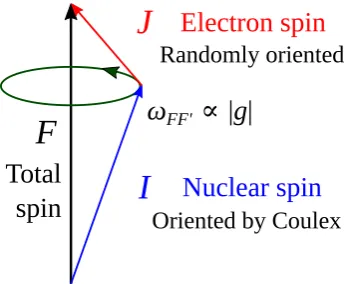
The RIV technique can be used to measure the nuclear gfactor via a perturbation of theγ-particle angular correla-tion arising from the nuclear-electronic dipole interaccorrela-tion [3]. When ions recoil in vacuum the electron spins (J) are presumed to have no preferred orientation in space, whereas the nuclear spins (I) have been oriented by the Coulomb excitation. The nuclear and electron spins then couple and, in the vector model picture, begin to precess about their total spin (F) at a frequency proportional to theg factor. This interaction is illustrated in Fig. 1. For a single, static atomic state, the periodic de-alignment and
I
J
Randomly oriented
Oriented by Coulex
F
ω
FF'∝
|
g
|
Nuclear spin
Electron spin
Total
spin
Figure 1. Spin coupling between the nuclear (I) and electron (J) spins, combining such thatF=I+J. The dipole interaction results in a precession aboutFwith angular frequencyωFF0[see Eq. (2)].
re-alignment of the nuclear spin perturbs the angular corre-lation. This appears as an alternate attenuation and restora-tion in the anisotropy of the angular correlarestora-tion as a cosine function. The periodic attenuation factor [3] is
Gk(t)= X
F,F0
(2F+1)(2F0+1) 2J+1
(
F F0 k
I I J
)2 e−iωFF0t.
(1) wheretis time, the quantum spin numbers have their es-tablished designation, the curly braces signify a Wigner 6-Jsymbol, and the precession frequency is
ωFF0= gBHF
2J µN
~
[F(F+1)−F0(F0+1)]. (2)
where BHF is the hyperfine-field strength (which can be calculated from atomic theory), andµNis the nuclear mag-neton. Note that wFF0 varies for eachF,F0coupling, re-sulting in a superposition of different frequencies when J>1/2.
When multiple atomic states contribute in sequence, their effect is multiplicative. Alignment lost through pre-cession of a prior state is never regained, fixing a new max-imum alignment. The average attenuation coefficient for an individual charge stateGAQk , resulting from atomic de-cays through a sequence of states, is thus
GAQk (tN)=G1k(t1) N Y
i=2
G(ki)(ti−ti−1). (3)
whereAandQrepresent the atomic-decay sequence and charge state, respectively,G(ki)is the attenuation coefficient in statei,tiis the time at which the state decayed, andNis the total number of states in the decay cascade up to time tN.
Generally, there will be a distribution of charge states, each contributing a large number of atomic decay se-quences with their own resultingGAQk . Hence, the average contribution ofGkAQfor each charge state must be consid-ered. The value obtained when averaging across a charge-state distribution ¯Gkis determined by
¯ Gk(t)=
NQ
X
Q cQ
NA
X
A
GAQk (t)/NA. (4)
whereNA is the number of atomic-decay chains in an in-dividual charge state, NQis the number of charge states, andcQis the fractional population of an individual charge state.
2.3 Attenuation ofγ-particle angular correlations
to the E2 matrix elements. The angular correlation [18] can be calculated by
W(t, φ, θ)=X k,q
√
2k+1ρkqGk(t)FkQkDkq∗0(φ, θ,0). (5)
wherek=0,2,4 and−k≤q≤k,ρkqis the statistical tensor defining the spin alignment of the excited nuclear state, Gk(t) is the attenuation coefficient, Fk represents the F-coefficients for theγ-ray transition [17],Qkis the attenu-ation factor due to the finiteγ-ray detector size, andDkq0 is the WignerDrotation matrix [17]. The anglesφandθ are spherical polar coordinates, where the position of the beam spot on the target represents the origin, and the beam direction defines thezaxis.φis the relative azimuthal an-gle between the γ-ray detector and the particle detector, andθis the polar angle of theγ-ray detector.
The time-dependent attenuation coefficient,Gk(t), can be measured using a plunger device, which quenches the hyperfine interaction at a particular distance (i.e after a set flight time) by implantation into a foil [19]. By measuring γ-particle coincidence events using a segmented, annular particle detector,θ- andφ-dependent angular correlations can be measured as a function of time.Gk(t) values can be obtained by fitting Eq. (5) to the data, withGk(k=2,4) as free parameters (G0=1). TheGkvalues can also be calcu-lateda priori, making thegfactor the only unknown pa-rameter. Atomic states having spinJ=1/2 are best suited to measuregfactors as they have a single cosine frequency over the summation ofF,F0. In our case Na-like ions, hav-ingJ=1/2 ground states, are the most useful charge state to populate.
2.4 Atomic structure calculations
To model the hyperfine interaction, the atomic structure in-formation of the charge states must be obtained. Progress in the field of atomic physics allows the calculation of atomic wavefunctions with great accuracy. One partic-ular solution for calculating atomic properties, the Gen-eral Relativistic Atomic Structure Package (GRASP), is freely available under the MIT license [20]. GRASP numerically solves the multiconfiguration Dirac-Hartree-Fock equations for atomic-state functions (ASFs) to ob-tain radial wavefunctions. AFSs are composed of a mix-ture of configuration-state functions (CSFs), defined by individual electron configurations. The vital point in us-ing GRASP is understandus-ing how the ASF is constructed. This is calculated by
Ψ(γPJ)= N X
i=1
ciΦ(γiPJ). (6)
whereΨis the ASF representing a physical atomic stateγ having parityPand angular momentumJ,Nis the number of chosen CSFs, with each CSFihaving a mixing coeffi -cientci, and a Slater determinantΦdefined by the electron configurationγi, parityPand angular momentumJ.
Equation (6) shows that any CSF having the same parity (P) and angular momentum (J) can contribute to
a given ASF. To obtain the most accurate solution, one would include CSFs up to the continuum states. How-ever, this is impractical as convergence becomes more dif-ficult and computation time becomes longer as the num-ber of CSFs increases. As such, one should choose CSFs that will have a significantci. Because we aim to simu-late spectral cascades, our approach has been to calcusimu-late ASFs having leading terms that are valence configurations. The CSFs chosen for these calculations allowed for dou-ble excitations from the core electrons, having principal quantum number n=2 or n=1 in this case, to improve transition-rate calculations. A single-electron excitation from the deep core (n=1) electrons was also allowed, to improve the hyperfine-field-strength calculation. CSFs were taken up to a value ofnwhere their number exceeded
∼106, at which point computation time was already quite long (∼1 week). The CSF space was increased by inter-vals ofn, with each new value adding a new electron shell. The ASFs were resticted to energy levels below 1000 eV, as per Ref. [10]. Once solutions were obtained, the cal-culated energy levels were compared to those in the US National Institute of Standards and Technology database for atomic spectra [21], and found to agree better than 1% in all cases, and 0.1% in most. This comparison is helpful in determining whether the radial wavefunctions have con-verged on an accurate solution. Another way convergence was assessed was to compare the results of the two oscil-lator strength calculation approaches (alternate forms for the dipole operator, or gauges) GRASP takes, namely the length and velocity forms [22]. Disagreement indicates the solution is not self-consistent. Most transitions were found to agree better than 1%, with poor agreement only observed for slow transitions between high-energy states, which were deemed unimportant in the present context due to the unlikeliness of their population or observation.
2.5 Monte-Carlo simulation
Finding an exact mathematical solution to the complex problem of calculating ¯Gk(t) is not practical. Instead, the Monte-Carlo method is used to obtain a solution by con-ducting a “virtual experiment” using the atomic structure calculations. For a given species an initial atomic state is selected at random following the chosen energy distribu-tion (e.g. Boltzmann or uniform). A nuclear survival time for the event is then generated by
tN(τN)=−loge(P)×τN. (7)
whereτN is the nuclear-state lifetime, andPis a random number evenly distributed between (0,1]. Then, the fol-lowing procedure is iterated (after initialising the cumula-tive atomic survival timetcto zero) :
1. If the atomic lifetime (τa) is finite, generate an atomic survival time (ta) for the atomic state as per Eq. (7), but withτa in place ofτN. Otherwise, set ta=tN−tcand end the event.
ta=tN−tcand end the event. Otherwise, addtato tc.
3. Select a new atomic state based on the transition probabilities.
Atomic levels andtavalues are recorded for each iteration. This procedure produces an event consisting of a number of atomic-level references and survival times, with a cu-mulative atomic survival time equal to the nuclear survival time. This information is then used to evaluate the atomic-state population through time, and once that is performed for each charge state, to calculate ¯Gk(t).
3 Results and Discussion
3.1 Charge-state distribution
Figure 2 shows the expected charge-state distribution of 56Fe ions in the ALTO measurement, centred on Na-like
ions. The distribution is quite broad, with the neighbour-ing Ne- and Mg-like species each comprisneighbour-ing∼70% of the Na-like population. In terms of atomic excitation, the Ne-like ground state will be dominantly occupied due to the closed electron shell. HavingJ=0, there will be no net hy-perfine interaction. The effect of this state on ¯Gk(t) will be to reduce the amplitude of the Na-likeJ=1/2 cosine fre-quency. The Mg-like species will have many populated ex-cited atomic states, close in energy, due to having two va-lence electrons. The hyperfine interaction in such species appears as a quasi-exponential attenuation through time, again effectively reducing the Na-like cosine frequency amplitude. The effect is the same for the Al-like charge state. The single-hole F-like ions have low-energy, long-lived atomic states with hyperfine-field strengths similar to the Na-like atomic states. If they are strongly populated, the resulting interference patterns may be difficult to de-convolute.
3.2 Atomic-state populations
Monte-Carlo simulations, using the calculated atomic en-ergy levels and transition rates, were used to explore how the population of atomic states could vary through time.
Figure 2.Estimated charge-state distribution of56Fe ions in the TDRIV measurement at ALTO.
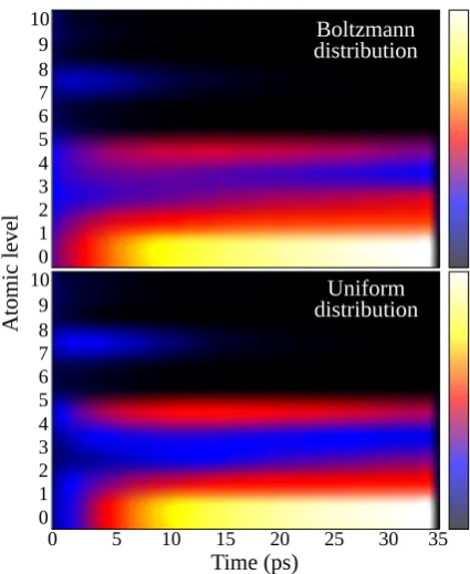
These populations obviously depend on the initial distri-bution of atomic states, which is not well known. A com-parison of the atomic population distributions for Na-like 56Fe ions with time, one having an initial population with a
Boltzmann energy distribution of mean energyT=100 eV, and the other a uniform distribution up to the highest-energy ASF, is shown in Fig. 3. Both initial distributions populate similar atomic states at longer times (>25 ps), but have different relative intensities on the order of the nuclear lifetime (10 ps). The initial Boltzmann distribu-tion results in low-energy states being preferentially popu-lated from early time points, with the ground state having a dominant contribution from t=0. Feeding cascades from higher-energy states are also much less influential.
Of the five charge states present, only two have atomic states with observable frequencies: Na-like and F-like. Figure 3 shows that irrespective of whether a Boltz-mann or uniform initial distribution is chosen, for Na-like ions three low-lying atomic states, 3s1/2(0), 3p1/2(1) and 3d5/2(4), where the numbers in parentheses are the state labels in Fig. 3, are rapidly (<5 ps) populated. Of these three, only the 3s1/2 and 3p1/2 states have observ-able frequencies. In F-like ions, proximity to the neon shell-gap results in the ground and first-excited state (2p3/2 and 2p1/2holes) being dominantly populated within a few picoseconds, and both have observable frequencies. For
0 5 10 15 20 25 30 35 10
9 8 7 6 5 4 3 2 1 0
Atomic leve
l
Time (ps)
10 9 8 7 6 5 4 3 2 1 0
Boltzmann distribution
Uniform distribution
1.0 0.8 0.6 0.4 0.2 0 -0.2 -0.4 -0.6 0.8 0.6 0.4 0.2 0 -0.2 -0.4 -0.6
0 5 10 15 20 25 30 0 5 10 15 20 25 30 35
Time (ps)
Gk
(
t
)
G2
G4
(a) (b)
(c) (d)
Figure 4. IndividualGk(t) plots for Fe ion (a) F-like 2p3/2, (b) F-like 2p1/2, (c) Na-like 3s1/2, and (d) Na-like 3p1/2. These are all evaluated withg(2+1; Fe56)=0.51, as previously reported [23].
these four atomic states, the pureGkvstplots of their in-dividual frequencies are shown in Fig. 4.
3.3 Fitting thegfactor
MeasuredGk(t) values were obtained by fitting Eq. (5) to the data as described in Section 2.3. For clarity of analysis, a subset of the total data was chosen. This subset was taken by the ORGAM array (having high statistics) and rejected γ-rays emitted by nuclei which had decayed in flight. By varying thegfactor used in the calculation of ¯Gk(t) from the Monte-Carlo simulation events, an optimal fit to the data points can be found. Another important fit param-eter is the distribution of atomic states, as this will affect the observed frequencies and the average magnitude of the
¯
Gkvalues. Presently, this parameter is poorly understood. Because of this, it is illuminating to instead consider, indi-vidually, the major contributing atomic states, and whether they have frequencies that will appreciably affect the mea-surement. The atomic-state-population heatmaps (Fig. 3), instead of reproducing the measured data, were used to help identify significantly contributing states. A frequency superposition of these states then allowed grand features of the measuredGk(t) values to be probed by varying their population. If these features of theGkvstplot can be un-ambiguously reproduced, then thegfactor can be robustly determined.
The measuredGk(t) values are shown in Fig. 5 along with a fit using only the frequencies shown in Fig. 4. Fo-cusing on the experimental data points, there are two no-table features: the peak-like increase inGkat 16 ps, and the broader increase at 25 ps. By reference to Fig. 4, the interference pattern between the F-like 2p1/2 and the Na-like 3s1/2frequencies produces a constructive peak at 16 ps, but interferes more destructively elsewhere. This near-cancellation can explain the smoother variation from 6 to 10 ps, and 23 to 27 ps. Both the F-like 2p3/2and the
Na-like 3p1/2frequencies can contribute to the increase in Gkat 25 ps, but the Na-like 3p1/2frequency appears to be dominant. Additionally, the different effective frequencies forG2 andG4from the F-like 2p3/2 state, resulting from its J =3/2 atomic spin, can explain the proximity ofG2 andG4values near 10 ps and 20 ps. The frequency super-position in Fig. 5 was made to be in line with the mea-sured charge state distribution and predicted atomic-state populations, and to reproduce the peaks at 16 ps and at 25 ps. Fitting these features givesg≈0.55, different from the literature value indicated in Fig. 4, but consistent with it, within experimental uncertainty. Changinggby more than±0.02 causes significant misalignment of the fit from these prominent features.
When attempting to fit the entire timespan, the data seem to show a changing relative population of states through time. Initially, a strong relative contribution from the F-like states matches the initial rapid decrease, with the 2p3/2 state’s frequency responsible for the proximity of G2 andG4 around 10 ps. After this point, increasing population of the Na-like states relative to the F-like states matches the sharp peak at 16 ps, and their continued pop-ulation increase is required to bring about the large peak at 25 ps. A plausible explanation is that, initially, higher-energy excited atomic states are strongly populated in the Na-like ions, and then decay to the low-energy states. However, Monte-Carlo simulations have so far been un-able to accurately reproduce this behaviour. This hypoth-esis is currently under investigation. The complicated su-perposition of changing populations makes a global fit dif-ficult. Preliminary results from a global fit indicate that the gfactor could possibly be determined with an uncertainty below±0.01. It should be noted, however, that systematic sources of uncertainty are yet to be quantified, with the
1.0
0.8
0.6
0.4
0.2
0
-0.2
-0.4
0 5 10 15 20 25 30 35
Time (ps)
Gk
(
t
)
G2
G4
G2 fit
G4 fit
most significant expected to be the uncertainty in the abso-lute time offset (plunger zero-distance). However, even at this stage of analysis, fitting of major trends can evidently provide a robust measure of thegfactor.
It should be clarified that G2 andG4 are highly cor-related, so free-fitting by χ2 minimisation may not give correct relative magnitudes. It will, however, reveal fre-quency trends that are useful in guiding the data analysis. As such, discrepancies in the magnitude of the fitted vs. measured values should not be considered too harshly at this preliminary stage. An approach by whichGk values are calculated a priori and fitted directly to the angular correlation, while also allowing atomic-state populations to vary in time realistically, is in progress.
4 Conclusion
The TDRIV measurement technique has been demon-strated as a promising way to measure g(2+1) values in short-lived nuclear states of radionuclides. Detailed Monte-Carlo simulations based on atomic-structure calcu-lations reveal that multiple atomic states contribute to the hyperfine interaction for nuclei around Z=30, creating a superposition of frequencies. By modelling and fitting the population of states through time, it appears that theg fac-tor can be reliably determined. The relevant hyperfine in-teraction frequencies from a TDRIV data set on56Fe were identified and suggestg≈0.55, with an accuracy of∼4%. An improved data analysis technique is being developed, from which preliminary results indicate that theg factor could be determined with close to 1% precision, the fi-nal precision likely dependent on systematic uncertainties associated with the plunger technique as much as the mod-elling of the hyperfine fields.
Acknowledgements
The authors are grateful to the academic and technical staff of the IPN ALTO facility and the ANU HIAF for their as-sistance and maintenance of the facilities. In particular, the authors would like to thank J. Ljungvall, I. Matea, T. Konstatinopoulos, K. Gladnishki, A. Gottardo and D. Yor-danov for their assistance with the data collection. This research was supported in part by the Australian Research Council under grant number DP170101673. A. G. ac-knowledges the support of the P2IO Excellence Labora-tory. B. P. M. acknowledges the support of the Australian Government Research Training Program. Support for the ANU Heavy Ion Accelerator Facility operations through the Australian National Collaborative Research Infrastruc-ture Strategy (NCRIS) program is acknowledged.
References
[1] N. Benczer-Koller and G. J. Kumbartzki, Journal of Physics G: Nuclear and Particle Physics34, R321 (2007).
[2] A. E. Stuchbery, Hyperfine Interactions 220, 29 (2013).
[3] G. Goldring, in Heavy Ion Collisions, edited by R. Bock (North-Holland Pub. Co., 1982), Vol. 3, p. 483.
[4] N. J. Stone, A. E. Stuchbery, M. Danchev, et al., Phys. Rev. Lett.94, 192501 (2005).
[5] J. M. Allmond, A. E. Stuchbery, D. C. Radford,et al., Phys. Rev. C87, 054325 (2013).
[6] A. E. Stuchbery, J. M. Allmond, A. Galindo-Uribarri, et al., Phys. Rev. C88, 051304(R) (2013).
[7] A. E. Stuchbery, J. M. Allmond, M. Danchev,et al., Phys. Rev. C96, 014321 (2017).
[8] A. Kusoglu, A. E. Stuchbery, G. Georgiev, et al., Phys. Rev. Lett.114, 062501 (2015).
[9] A. E. Stuchbery and N. J. Stone, Phys. Rev. C76, 034307 (2007).
[10] N. J. Stone, J. R. Stone and P. Jönsson, Hyperfine Interactions197, 29 (2010).
[11] X. Chen, D. G. Sarantites, W. Reviol and J. Snyder, Phys. Rev. C87, 044305 (2013).
[12] J. Ljungvall, G. Georgiev, S. Cabaret, et al., Nucl. Inst. Meth. A679, 61 (2012).
[13] C. Le Galliard, Tech. rep., IPN Orsay, IPN Orsay, University of South Paris, Orsay, France (2019),
http://ipnwww.in2p3.fr/Orgam?lang=en. [14] N. Warr, J. Eberth, G. Pascovici,et al.,MINIBALL:
A Gamma-ray spectrometer for exotic beams(2003). [15] A.E. Stuchbery, A.B. Harding, D.C. Weisser, N.R. Lobanov, Nucl. Instrum. Methods Phys. Res. A951, 162985 (2020).
[16] A. E. Stuchbery and M. P. Robinson, Nucl. Instrum. Meth. Phys. Res. A485, 753 (2002).
[17] K. Alder, A. Winther, Electromagnetic excitation: theory of Coulomb excitation with heavy ions (Ams-terdam: North Holland, 1975).
[18] A. E. Stuchbery, Nuclear Physics A723, 69 (2003). [19] A. Kusoglu, A.E. Stuchbery, G. Georgiev, et al., J.
Phys. C590, 012041 (2015).
[20] C. Froese-Fischer, G. Gaigalas, P. Jönsson, J. Biero´n, Computer Physics Communications237, 184 (2019). [21] Y. Ralchenko, NIST Atomic Spectral Database pp. https://www.nist.gov/pml/atomic–spectra–database (2019).
[22] C. Froese-Fischer, T. Brage and P. Jönsson, Com-putational Atomic Structure: An MCHF Approach (Inst. Phys. Pub. Bristol and Philadelphia, 1997). [23] M. C. East, A. E. Stuchbery, S. K. Chamoli, et al.,