University of Windsor University of Windsor
Scholarship at UWindsor
Scholarship at UWindsor
Electronic Theses and Dissertations Theses, Dissertations, and Major Papers
2009
Analysis of scheduling in a diagnostic imaging department: A
Analysis of scheduling in a diagnostic imaging department: A
simulation study
simulation study
Brendan Eagen
University of Windsor
Follow this and additional works at: https://scholar.uwindsor.ca/etd
Recommended Citation Recommended Citation
Eagen, Brendan, "Analysis of scheduling in a diagnostic imaging department: A simulation study" (2009). Electronic Theses and Dissertations. 7976.
https://scholar.uwindsor.ca/etd/7976
ANALYSIS OF SCHEDULING IN A DIAGNOSTIC IMAGING DEPARTMENT:
A SIMULATION STUDY
By
Brendan Eagen
A Thesis
Submitted to the Faculty of Graduate Studies through Industrial and Manufacturing Systems Engineering
in Partial Fulfillment of the Requirements for the Degree of Master of Applied Science at the
University of Windsor
Windsor, Ontario, Canada
2009
1*1
Library and Archives CanadaPublished Heritage Branch
395 Wellington Street Ottawa ON K1A0N4 Canada
Bibliotheque et Archives Canada Direction du
Patrimoine de I'edition 395, rue Wellington OttawaONK1A0N4 Canada
Your file Votre reference ISBN: 978-0-494-57622-9 Our file Notre inference ISBN: 978-0-494-57622-9
NOTICE: AVIS:
The author has granted a
non-exclusive license allowing Library and Archives Canada to reproduce,
publish, archive, preserve, conserve, communicate to the public by
telecommunication or on the Internet, loan, distribute and sell theses
worldwide, for commercial or non-commercial purposes, in microform, paper, electronic and/or any other formats.
L'auteur a accorde une licence non exclusive permettant a la Bibliotheque et Archives Canada de reproduire, publier, archiver, sauvegarder, conserver, transmettre au public par telecommunication ou par I'lnternet, preter, distribuer et vendre des theses partout dans le monde, a des fins commerciales ou autres, sur support microforme, papier, electronique et/ou autres formats.
The author retains copyright ownership and moral rights in this thesis. Neither the thesis nor substantial extracts from it may be printed or otherwise reproduced without the author's permission.
L'auteur conserve la propriete du droit d'auteur et des droits moraux qui protege cette these. Ni la these ni des extraits substantiels de celle-ci ne doivent etre imprimes ou autrement
reproduits sans son autorisation.
In compliance with the Canadian Privacy Act some supporting forms may have been removed from this thesis.
Conformement a la lot canadienne sur la protection de la vie privee, quelques formulaires secondaires ont ete enleves de cette these.
While these forms may be included in the document page count, their removal does not represent any loss of content from the thesis.
Bien que ces formulaires aient inclus dans la pagination, il n'y aura aucun contenu manquant.
Author's Declaration of Originality
I hereby certify that I am the sole author of this thesis and that no part of this thesis has been
published or submitted for publication.
I certify that, to the best of my knowledge, my thesis does not infringe upon anyone's copyright
nor violate any proprietary rights and that any ideas, techniques, quotations, or any other material from
the work of other people included in my thesis, published or otherwise, are fully acknowledged in
accordance with the standard referencing practices. Furthermore, to the extent that I have included
copyrighted material that surpasses the bounds of fair dealing within the meaning of the Canada
Copyright Act, I certify that I have obtained a written permission from the copyright owner(s) to include
such material(s) in my thesis and have included copies of such copyright clearances to my appendix.
I declare that this is a true copy of my thesis, including any final revisions, as approved by my
thesis committee and the Graduate Studies office, and that this thesis has not been submitted for a
higher degree to any other University or Institution.
Abstract
In this thesis we present an Agent-Based Modelling Tool (ABMT) for use in the investigation of
the impact that operational level changes have on diagnostic imaging scheduling and patient wait times.
This tool represents a novel application of agent-based modelling in the outpatient scheduling /
simulation fields. The ABMT is a decision support tool with a user friendly graphical user interface that is
capable of modelling a wide array of outpatient scheduling scenarios. The tool was verified and
validated using data and expertise from Hotel Dieu Grace Hospital, Windsor, Ontario, Canada. The ABMT
represents a technological advancement in the modelling of multi-server, multi-priority class customer
Dedication
To my parents,
Acknowledgements
Dr. Richard Caron
Dr. WalidAbdul-Kader
Kathy Hillman
Gail Peterson
Mary-Alice Beneteau
Neil McEvoy
Dayna Roberts
Dave McKenzie
Jacquie Mummery
Table of Contents
Author's Declaration of Originality iii
Abstract iv
Dedication v
Acknowledgements vi
List of Tables ix
List of Figures x
List of Acronyms xi
1. Introduction 1
1.1 Problem Description 2
1.2 Thesis Statement 3
1.3 Objectives 3
1.4 Research Methodology 3
2. Review of Literature 5
2.1 Queueing Theory 5
2.2 Simulation 8
2.2.1 Simulation Paradigm 9
2.2.2 Agent-Based Simulation 11
2.2.3 Simulation in Healthcare 11
2.3 Outpatient Scheduling and Simulation 12
2.4 Literature Review Conclusions 18
3. Agent-Based Modelling Tool (ABMT) 19
3.1 ABMT Environment 19
3.2 Patients 22
3.3 Scheduling Discipline 23
3.4 User Interface 26
3.4.1 Setup & Go 26
3.4.2 Data Recording 26
3.4.3 Random Fill 26
3.4.4 Simulation RunTime 26
3.4.5 Number of Servers 26
3.4.6 Scheduled Hours per Day 26
3.4.7 Information Display 26
4. Case Study: Hotel Dieu Grace Hospital 29
4.1 Scheduling Process 29
4.2 ABMT Parameters 29
4.2.1 Arrival Rates 29
4.2.2 Operating Hours & Number of Scanners 30
4.2.3 Prebooked Periods 30
4.3 Acquired Data 30
5. Verification and Validation 32
5.1 Simulation Parameters 32
5.2 Discussion of Simulated vs. Historical Data 35
6. Discussion 36
7. Conclusions and Future Work 38
Bibliography 40
Appendix I: NetLogo™ Code for ABMT 44
List of Tables
Table 1 - Westeneng's Input Parameters from Outpatient Scheduling Survey 13
Table 2 - Westeneng's control parameters and mechanisms from Outpatient Scheduling Survey 14
Table 3 - Comparison of ABMTto published works 15
Table 3 Continued - Comparison of ABMTto published works 16
Table 3 Continued -Comparison of ABMTto published works 17
List of Figures
Figure 1 - Single Stage, Multi-Server Queueing System 6
Figure 2 - Approaches (Paradigms) in simulation modelling on abstraction level scale 10
Figure 3 - Patches andTurtle 19
Figure 4 - Layout of Simulation Environment 20
Figure 5 - Multi-Server Layout 20
Figure 6 - PrebookedTime 21
Figure 7 - Prebooked Time Control 21
Figure 8 - Arrival Distribution Control 22
Figure 9 - Scheduling Process: Single Server 23
Figure 10 - Scheduling Process: Multi-Server 24
Figure 11 - Bumping: Before and After 25
Figure 12 - Information Display 27
Figure 13 - Comparison of Service Request by Month and Class 31
Figure 14- Comparison of Wait Times by Month and Class 31
Figure 15 - Requests for Service by Class - April 07 to May 09 31
Figure 16 - HDGH Prebooked Schedule 33
Figure 17 - Simulated Wait Times for Class 4 Patients 34
Figure 18 - Simulated Wait Times for Class 3 Patients 34
Figure 19 - Simulated Wait Times for Class 2 Patients 34
Figure 20 - Average Wait Time for Class 4 Patients 35
List of Acronyms
ABMT-Agent-Based Modelling Tool
CAT - Computed Axial Tomography
CT - Computed Tomography
FCFS - First Come First Serve
GUI - Graphical User Interface
HDGH - Hotel Dieu Grace Hospital
LHIN - Local Health Integration Network
MRI - Magnetic Resonance Imaging
SIRO - Service In Random Order
1. Introduction
Canada's publicly funded healthcare system is dynamic. The system, composed of 10 provincial
and 3 territorial plans, has evolved into its current state over the past forty years. The goal of the system
however remains unchanged; providing universal coverage for medically necessary healthcare services
on the basis of need rather than the ability to pay. In recent years stress on the system has been
increasing due to factors such as the high cost of new medical technology and the aging of the baby
boom generation (Ministry of Health, 2005). In years to come this stress will only continue to increase as
the number of senior citizens in Canada continues to climb. The percentage of the total population that
were senior citizens in 2005 was 13%, however by 2036 that number is expected to nearly double to
24.5% (Turcotte & Schellenberg, 2006). Combined with the fact that seniors historically have consumed
44% (Canadian Institute for Health Information, 2008) of the healthcare spending of provinces and
territories it's plain to see that Canadian healthcare system is headed into a period that will tax its
resources to a new level.
One area where resources are already spread thinly is diagnostic imaging. This area is concerned
with the use of MRI (Magnetic Resonance Imaging), CT or CAT Scans (Computed Axial Tomography),
Ultrasounds and X-Rays. In 2004 there were on average 4.9 MRI machines and 10.2 CT Scanners for
every million Canadians; by 2007 those numbers had risen to 6.8 and 12.8, respectively (Canadian
Institute for Health Information, 2004) (Canadian Institute for Health Services, 2007). However, between
2006 and 2007 the demand for MRI and CT scans increased by 42.9% and 27.9%, respectively.
Compounding this issue is the fact that diagnostic imaging resources are not evenly distributed across
the country, for example by the end of 2006 there were 10.2 CT scanners per million people in Ontario
but 21.6 per million people in Newfoundland and Labrador (Canadian Institute for Health Information,
2007). As a result of the increasing demand for and uneven distribution of diagnostic imaging equipment
wait times for diagnostic imaging scans have become a concern in Canada. To that end the government
of Ontario has begun an initiative to track wait times in areas throughout the province
(http://www.health.gov.on.ca). The Ministry of Health has also established target wait times for patients
of different acuity (sickness) levels which are used to assess healthcare providers' wait time
performance.
At present, in many areas of Canada, the demand for diagnostic imaging services outstrips the
ability of public healthcare to provide these services. As a result, requests for services can go unmet,
The 'Wait Time' targets established by the government of Ontario represent the maximum period a
particular class of patients can wait for service before their health will suffer. At present there are 4
categories of patient acuity; class 1 patients are the sickest and require immediate attention (within 1
day) whereas class 4 patients are less critical and can often be elective requiring attention within 28
days.
The focus of this study will be 'Wait Time' as described by provincial government of Ontario's
guidelines. However, from a queueing theory perspective this is not the actual wait time, but can be
more accurately described as access time. The key difference being that this thesis will examine the days
between the request for service and the day of service and will not consider the time that a patient may
wait for service on the day that he or she is scheduled as a result of interruptions in the pre-established
schedule. Essentially, the thesis will ignore the fact that a patient may have to wait as long as the waiting
occurs on the day that the patient is scheduled to be scanned. It should be noted that in many works
the terms access time and wait time are used interchangeably, we will assume them to both mean the
number of whole days a patient waits between requesting and undergoing service.
Based on these factors it is plain to see that diagnostic imaging service providers will need a
means to effectively manage resources, allocate funds and control their processes if they are to cope
with the increasing demand of the Canadian population for their services to be delivered in a timely
manner.
1.1 Problem Description
It was the recognition of the reality facing a diagnostic imaging department that lead to the
conception of this thesis. The research team, which consisted of Dr. Richard Caron, Dr. Walid
Abdul-Kader and Mr. Brendan Eagen, was invited by Mr. Neil McEvoy, former CEO of Hotel Dieu Grace Hospital
(HDGH), Windsor, Ontario, Canada, to study his hospital's diagnostic imaging department and its
scheduling system. As a trained industrial engineer Mr. McEvoy was keenly aware of the benefits of
simulation and requested that the team pursue an agent-based solution to the problem. His vision was
that a tool be created for him and his staff that would assist them in the evaluation of the effects of
operational level changes to their current system. Mr. McEvoy suggested the use of NetLogo™, a zero
cost software used by researchers interested in agent-based modelling. These directives motivated this
thesis.
1.2 Thesis Statement
Our thesis is that agent-based modelling can provide a technological tool for use by hospital decision
makers to evaluate the effects that operational level changes will have on their diagnostic imaging
system with specific interest in the impact the changes will have on patient scheduling and wait time.
1.3 Objectives
With the above thesis statement in mind the objectives of this thesis are to create an
agent-based simulation tool with an easy to understand graphical user interface (GUI) that would allow
hospital decision makers to assess the impact of potential operational level changes to the diagnostic
imaging department on the department's schedule of patients. Additionally this thesis will expand
knowledge of the use of agent-based modelling in the outpatient scheduling field. The tool is a decision
support tool, not a model of any one specific diagnostic imaging department, and allows users to modify
input parameters according to the scheduling system that they wish to model.
1.4 Research Methodology
The research methodology is implicit in the following overview of the thesis layout. Though enumerated,
many of the outlined activities were carried out in parallel.
1. Preliminary Research
a. Review of literature - An exhaustive literature review was performed and the results
provided insight into the proposed research's place in the fields of healthcare
simulation/scheduling and agent-based modelling. In the case of HDGH scheduling is
taken to mean the assignment of a patient to a specific appointment slot on a particular
CT scanner. Additionally, the literature review helped to establish the parameters that
would be used in the construction of the simulation model.
b. Consultation with healthcare professionals - Consultation with practicing medical
professionals and healthcare administrators helped to establish the user interface
requirements of the model as well as providing insight into what internal and external
factors affect the scheduling process.
2. Design and development-The model was developed in the NetLogo™ simulation package using
the parameters established in the Preliminary Research phase. In order to use the NetLogo™
control it. Learning this programming language required several months of study and resulted in
the development of a prototype simulation model designed to simulate scheduling of a single
server. Once the programming language had been mastered, the prototype model was
expanded to accommodate multi-server scenarios.
3. Verification and Validation - The model was presented to medical professionals and healthcare
administrators to verify that the diagnostic imaging scheduling process was accurately
represented in the model. Historical data was collected from the sponsoring hospital, HDGH,
and used to validate the simulation results.
4. Discussion - The overall effectiveness of the simulation tool was assessed and observations
were made and documented regarding the applicability of agent-based simulation to scheduling
in healthcare.
5. Dissemination - The simulation tool will be shared with Canadian medical professionals,
healthcare administrators and healthcare researchers.
2. Review of Literature
This review of literature assists in the determination of what methodology should be used to
approach the topic of this thesis and also to determine the thesis' place in published literature. The
researchers will first consider the macro level problem of what solution method they wish to use. The
end result of this thesis will be a decision support tool that is transportable between diagnostic imaging
scheduling systems, as this decision support system will be required to support a system that is
relatively complex and also relies heavily on historical data thus a simulation-based decision support
system appears appropriate. Examples of simulation successfully being applied in healthcare include the
work of (McClean & Millard, 1995), (Everett, 2002) and (Aktas, Ulengin, & Sahin, 2007) who have all
effectively applied simulation-based decision support in healthcare. Everett gives perhaps the best
justification for choosing simulation as a decision support tool. He states that the complex web of
stakeholder objectives in healthcare all but precludes the existence of an "optimal" solution to a
problem. Instead he suggests that it is the system modeller's job to enable informed debate among
stakeholders. To that end, he continues, the development of a simulation model for decision support is
an excellent means by which to encourage communication between stakeholders and the modeller so
as to accurately capture the true nature of the system. Simulation also, through use of a graphical user
interface, allows the stakeholders without technical backgrounds to contribute to the development and
assume ownership and commitment to the model. It should be noted that simulation was not the only
option considered for modelling the diagnostic imaging scheduling system. Queueing theory / analytical
options were initially considered but the complex nature of the system combined with the need for
flexibility across a wide array of scenarios lead us to disregard these approaches.
2.1 Queueing Theory
Based on preliminary consultations with HDGH diagnostic imaging staff we determined that the
system can most readily be compared to a queueing system in which multiple servers work in parallel to
serve a single queue of customers with weighted priority on a first come first serve basis and that have
deterministic service times. Figure 1 depicts a single-stage queueing system with multiple servers in
Customers
(Infinite Queue)
Servers
(Multiple Servers in Parallel)
SI
S2
S3
N
Figure 1 - Single Stage, Multi-Server Queueing System
Although discounted as a solution to this particular problem, queueing theory still provides a
useful means by which to describe the situation under consideration.
In order to understand queueing theory notation and its ability to describe the current problem
one must be familiar with the basic components of a queue and the way in which it functions. A brief
overview of queueing as well as the importance of the exponential distribution is provided by (Winston,
2004). A queue is essentially a waiting line in which customers wait to receive service from a server.
Queueing theory helps one to describe and understand the relationships between customers, queues
and servers.
Customers, be they people, automobiles, manufacturing equipment, etc. require 'service' of
some sort. For example, people are serviced at a bank or in a grocery store, cars are serviced by a
mechanic and a broken welding robot is serviced by a technician. In these cases the number of
customers often exceeds the number of servers, that is, the number of people requiring banking
services exceeds the number of bank tellers for example. In situations such as there queues form. The
order in which customers in a queue are serviced by the servers is known as the queue discipline. The
most common queue discipline is First Come First Serve but others exist such as Last Come First Serve
and Service In Random Order.
Understanding how customers come to be in the queue is another important aspect of queueing
system. The rate at which customers arrive is known as the 'arrival rate' and in general can be modelled
by a mathematical distribution, the most common of which is the exponential distribution.
Exponential distributions are used to model interarrival times because of their no-memory
property. That is,
P(A>t + h nA >t) e-^t+K> ..
P(A>t + h\A>t) = p { A^t ) >-=——= e-*=PiA>h)
"The no-memory property of the exponential distribution is important, because it implies that if we
want to know the probability distribution of the time until the next arrival, then it does not matter how
long it has been since the last arrival." (Winston, 2004)
Other factors also affect the arrival process such as whether or not more than one customer can arrive
in the system at a time and also the total number of customers that the system services.
Modelling the time required for a customer to receive service is also a key element of queueing
theory. The Erlang distribution is commonly used to model services times, however, other distributions
are also common. In some cases, when the same actions are repeated for every customer, the service
time will always be the same. In these situations the service time is said to be deterministic.
In order to summarize all of the information required to describe a queue Kendal developed a
standard notation (Kendall, 1951). Known as the Kendall notation, this method describes queues based
on 6 characteristics.
1) The arrival process
2) Service times
3) # of parallel servers
4) Queue discipline
5) Max. # of customers in the system
6) Size of the population
Standard abbreviations were assigned to each characteristic, for example, M denotes an exponential
Thus,
M / D / 2 / FCFS / «=> /oo
denotes a queueing system whose customers arrive based on an exponential distribution of interarrival
times which are served by two servers at a deterministic rate in a first come first serve manner. The
customers come from an infinite supply and are unlimited in the number that can occupy the system.
While a model of the imaging department at HDGH as an M/D/2/FCFS/00/00 queue might
provide insight, it would fail to capture complexities such as multiple patient classes that cause a
violation of the FCFS queue discipline; and scanner downtime so that the servers are not continuously
available. This reasoning leads us to the conclusion that simulation would be a better modelling
technique.
2.2 Simulation
Simulation is the imitation of the operation of a real-world process or system over time (Banks et al,
2005). Simulation can provide a means by which to forecast the future of the diagnostic imaging
schedule based on those past known events. The benefits of simulation are many fold as presented by
(Shannon, 1992):
• Simulation can be used to explore new policies, operating procedures, decision rules, organizational structures, information flows, etc. without disrupting the ongoing operations.
• New hardware designs, physical layouts, software programs, transportation systems, etc. can be tested before committing resources to their implementation.
• Hypothesis about how or why certain phenomena occur can be tested for feasibility.
• Simulation allows us to control time. - Time can be easily compressed, expanded etc. allowing us to quickly look at long time horizons or to slow down a phenomenon for study.
• Simulation can allow us to gain insight into which variables are most important to performance and how these variables interact.
• Simulation allows us to identify bottlenecks in material, information and product flows.
• The knowledge gained about a system while designing a simulation study may prove to be invaluable to understanding how the system really operates as opposed to how everyone thinks it operates.
Shannon's first point holds significant weight in the case of this thesis. It is not feasible or safe to
interrupt the current diagnostic imaging scheduling process as doing so may adversely affect the health
of the patients relying on the system. Many forms of simulation also have the added benefit of providing
the modeller with a visual representation of the system which can be useful when presenting the model
to those whose knowledge of the system or simulation is lacking (Banks et al, 2005).
2.2.1 Simulation Paradigm
The simulation field is composed of many different approaches or paradigms. A system can be
modelled in many different ways ranging from simulations performed by hand to complex
multi-scenario simulations that require more computing power than the average desktop PC has to offer. For
ease of calculation and timeliness this study focused on computer simulation. For the purpose of this
investigation we considered 3 central simulation paradigms; discrete-event simulation, agent-based
simulation and system dynamics simulation.
Discrete-event simulation can be described in terms of its components; entities, resources,
control elements and operations (Schriber & Brunner, 1997). Entities interact with system resources
based on the rules established by control elements to perform operations.
Agent-based simulation functions somewhat differently than discrete-event simulation. In
agent-based simulation agents are the primary focus. Agents are independent decision makers in a
system that react dynamically based on their characteristics and surroundings in a simulated
environment (Macal & North, 2007). Agent-based simulation is then the evolution of the behaviour of
the agents and their environment over time.
System dynamics simulation functions in a significantly different manner than discrete-event
simulation or agent-based simulation. System dynamics is primarily concerned with an aggregate level
of detail. It is not focused on individual entities or agents but aggregate behaviour of groups. It
functions by considering aggregate 'stocks' and their flow within a system based on feedback loops
(Coyle, 1996).
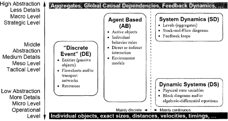
In Figure 2 (Borshchev & Filippov, 2004) provide a useful frame of reference for the simulation
paradigms considered. Figure 2 shows a comparison of the three paradigms with respect to their
appropriateness at various levels of abstraction. Borshchev and Filippov show that discrete-event
simulation is most appropriate at low to mid levels of abstraction in part due to its focus on individual
for modelling system with a high level of abstraction. In contrast to discrete-event and system dynamics,
agent-based simulation can be used across all levels of abstraction with the capability to model
operational level detail but also present high level trends accurately (Borshchev & Filippov, 2004). Based
on this information it appears safe to conclude that regardless of the level of abstraction that modelling
a diagnostic imaging scheduling process requires, agent-based simulation would be an acceptable tool.
High Abstraction Less Details Macro Level Strategic Level
Middle Abstraction Medium Details
Meso Level Tactical Level
Low Abstraction More Details Micro Level Operational
Level
ireqates. Global Causal Dependencies, Feedback Dynamics.
"Discrete Event" (DE)
- Entities (passive objj sets)
Flowcharts and/or transport networks Resources
Agent Based (AB)
• Active objects • Individual
behavior rules • Direct or indirect
interaction • Environment
models
Mainlv discrete •+
System Dynamics (SD)
• Levels (aggregates) • Stock-and-Flow diagrams • Feedback loops
Dynamic Systems (DS)
• Physical state variables « Block diagrams and/or
algebraic-differential equations
• Mainlv continuous
Individual objects, exact sizes, distances, velocities, timings,
Figure 2 - Approaches (Paradigms) in simulation modelling on abstraction level scale
The decision to use agent-based simulation was influenced in part also by Mr. McEvoy who felt that
this modelling technique might be especially applicable to diagnostic imaging scheduling and
recommended a free simulation software package, NetLogo™, to use in the modelling process.
Additionally, a preliminary review of literature revealed that using agent-based simulation to model an
outpatient scheduling system would be relatively novel. In support of this approach were (Macal &
North, 2007) who identify the appropriate time to use agent-based simulation with the following
criteria:
When there is a natural representation as agents
When there are decisions and behaviours that can be defined discretely (with boundaries) When it is important that agents adapt and change their behaviours
When it is important that agents learn and engage in dynamic strategic behaviours
• When it is important that agents form organizations, and adaptation and learning are important at the organization level
• When it is important that agents have a spatial component to their behaviours and interactions • When the past is no predictor of the future
• When scaling-up to arbitrary levels is important
• When process structural change needs to be a result of the model, rather than a model input
The diagnostic scheduling process meets the above criteria and so it was determined that agent-based
simulation would be an acceptable method to model the process. In the case of outpatient scheduling,
requests for appointments are considered agents and the schedule, represented on a 2 dimensional
plane (Time of the Day x Day in the planning horizon), is considered the environment.
2.2.2 Agent-Based Simulation
Agent-based simulation has a history in many fields including economics, mathematics, biology,
engineering, sociology and psychology (Axelrod, 2005). The application of agent-based simulation to
healthcare is a relatively novel but expanding field. However, much of that expansion is focused on
modelling the transmission of infectious diseases, such as the work of (Triola & Holzman, 2003) who
modelled the transmission of nosocomial diseases in intensive care units or (Teweldemedhin, Marwala,
& Mueller, 2004) who study the transmission of HIV.
2.2.3 Simulation in Healthcare
Although there is a limited amount of research that has employed agent-based simulation in
healthcare settings, there is a significant amount of research in healthcare using other forms of
simulation. This should not be taken to mean that agent-based simulation does not have a place in
healthcare; just that it is a relatively unexplored application. Although somewhat dated (Jun, Jacobson,
& Swisher, 1999) survey over one hundred publications which employ simulation in healthcare. The uses
of simulation they present are diverse including (but certainly not limited to) patient routing and flow
schemes (Garcia et al, 1995) (McGuire, 1994) (Blake, Carter, & Richardson, 1996) and bed sizing and
planning (Butler, Karwan, & Sweigart, 1992) (Lowery, 1992) (Dumas, 1985).
Of particular interest to this thesis were those publications focused on patient scheduling,
including the work of (Bailey, 1952) who contributed some of the earliest work in outpatient scheduling.
Outpatients are those patients who need to stay in the hospital overnight after visiting during the day.
Bailey, looking at outpatients, counterbalanced patient wait times with physician utilization, developing
helped pave the way for the application of a scientific approach to the study of outpatient scheduling.
(Smith, Schroer, & Shannon, 1979) continue in a similar vein with their work that considers maximizing
patients seen by a physician during a 3 hour session, while minimizing patient waiting time and
determining the required number of nurses and examination rooms needed.
2.3 Outpatient Scheduling and Simulation
For a more current look at simulation focused specifically on outpatient scheduling we turn to
(Cayirli & Veral, 2003) who survey outpatient scheduling and (Westeneng, 2007) who distils their work.
Westeneng presents a useful condensed version of Cayirli & Veral's outpatient scheduling survey as part
of his thesis on the evaluation of alternative appointment systems. His thesis shares commonalities with
this one but differs in its goals and approach. While this thesis focuses on a standard simulation tool for
outpatient scheduling in diagnostic imaging Westeneng focused on developing an optimal scheduling
procedure for a single ear, nose and throat clinic.
Westeneng presents Cayirli & Veral's work in two tables (See Tables 1 and 2). Table 1 captures
each works' input parameters; those parameters that are beyond the control of the simulator. These
parameters could also be called outside forces or factors as they act on their respective systems from
the outside, relatively uncontrolled by the system stakeholders (Note: Not all of the material referenced
by Westeneg could be located, however the table has been reproduced as it appears in his thesis). Table
2 presents the control factors and mechanisms imposed on each system. These are the variables of the
system that are available for manipulation by the simulator or the system stakeholder.
Westeneng's work served as a start point for establishing those internal and external
parameters that effect the operation of a diagnostic imaging scheduling system. While some parameters
are not applicable in the case of diagnostic imaging, others served to develop a deeper understanding of
the system when considered with the assistance of healthcare professionals and hospital decision
makers.
Input Parameters: Service Time Distribution
Patient Punctuality (mean, st.dev)
No-Shows (p = no-show probability)
Walk-Ins (regular
and emergency) Doctors' Lateness
Doctors' Interruption Level Articles: (Westeneng, 2007) (Bailey, 1952) (Blanco White & Pike)
(Cayirli, Veral, & Rosen, 2004) (Cayirli, Veral, &
Rosen, 2006) (Chen & Robinson,
2005) (Clague, Reed, Barlow, Rada, Clarke,
& Edwards, 1997) (Denton & Gupta,
2003) (Fetter & Thompson,
1966) (Fries & Marathe,
1981) (Harper & Gamlin,
2003)
(Ho, Lau, & Li, 1995) (Hutzschenreuter,
2004) (Kaandorp & Koole,
2007) (Klassen & Rohleder,
1996) (Klassen & Rohleder,
2004) (Lehaney, Clarke, &
Paul, 1999) (Liu & Liu, 1998) (Robinson & Chen,
2003) (Rohleder & Klassen,
2000) (Vanden Bosch, Dietz,
& Simeoni, 1999) (Vissers & Wijngaard,
1979) (Welch & Bailey,
1952) Gamma Gamma Gamma Lognormal Lognormal Randomly Randomly Uniform, Gamma and Normal Empirically collected Negative, Exponential Not specified Uniform, exponential Triangular, Gamma Exponential Lognormal Lognormal Not specified Uniform, exponential, Weibull Generalized Lambda Lognormal Erlang General Gamma N(-13, 17) Punctual Gamma, mu=0
N (-15, 25) N(0,25) and N
(-15,25) Unpunctual,
mu=0 Punctual
Punctual Late allowed to
max. 5 min. Punctual Unpunctual (mean 8.3 min early, SD=14.7 min) Punctual Unpunctual, (-10, 10) Punctual Punctual Punctual Punctual Punctual Punctual Punctual Punctual In system earliness Punctual
p = 0.05 p = 0 p = 0, 0.09 and
0.19 p = 0and0.15 p = 0and0.15
p = 0
p = 0, .2, .3
p = 0 p=[0.04-0.22] with mean 0.14
p = 0
p > 0(not specified)
p=0, 0.10, 0.20 p=0.10 p = 0,0.1, 0.25,
0.5 p = 0.05 p = 0.05 p = 0
p = 0, 0.10, 0.20
p = 0 p = 0.05
p = 0 Included by
adjusting service times
p = 0
Emergency only None None 0 to 15%, also
regular 0 to 15%, also
regular None
None
None 7 to 58% with mean
38% None Urgent None None None Max 2 emergencies
per session 10 % of patients
None
None
None Max. 2 emergencies
per session None Included by adjusting service times None
Late N(5,15) minutes Punctual 0,5, 10,15 or 20 min.
Punctual Punctual Punctual
Punctual
Punctual
0,30 or 60 min Punctual Unpunctual Punctual Punctual Punctual Punctual Punctual Punctual Uniform over [0,6]
min. late Punctual Punctual Punctual
In system earliness
Punctual yes (DICT) None None None None None None None None None None None None None None None yes None None None None None None
CQWR a PARAMETER S Msmmms Emmuss MO &sT clink Meyi1352 ) Banc o VVWe * Pik e (196* ) Cayirli , Vers ! SRase n (2004 ) Cetf it , Vera ! £ Ras« ! (208 ) CtenSRDfcritonpCiB ) asgwRal,n997 ) Dento n 3 Oypf a (208 ) Fstte r S ThomfiSCf i f1936 ) Frie s *Mar3the( 1 981 ) Harper * Gar * (20D3 ) Ho , Le w S i U (1355 ) HUiscfierwiisrp04 ) lteorpaK«fe(20e? 5 KteseftSRotederftSSS ) K!9sseftSRoh:e*r(200« ) Lsharev , CJarfe e S Pau l (1999 )
lu&uumm) R*;nso
n & Chsr « (2003 ) KohiederSKtesenPOi] ) Varde i Bosch , Kel i 8 Smeo-ni(1839 ) Vfeser s i Wjigow t (1979 ) V*ichSBsieyfi952 ) yetnodobs y
Simufetiar) SWatio
n Simulatio n SimiKfe n SimiMia n Analytica l SimiMo n Artytjqa l Simulator ! Ansfytica l Simulatio n Simulatio n SiffiiiaSiO n Arefyiica S Simulatio n Simulatio n Scft-simutetion ' Simiisiio n Analytica l Simiiatb n Analytica l Simuiaiio n Simulatio n SI M N-flterr f Sector s (Sj ; NUJtt e <5 J patisit s ps r sess w (N ) ai d D w sto i c f sessic n (T ; $=20 ; 7*15 ^ mm'r.,fi'/srles &=1 ; N= 1 a , 15,20.2 ^ T=12 5 »h . S*1;*ie,20,30,4Q,5Q.6fl t Ma * S=t;NM 0 &>1;^10,20,1=21 0 S=1;N= 2 S=3 ; *36-4 5 S=1;N-3,5. 7 S=3;N=2 8 S=1;Eu=2 4 S=22 , N ere f T ne t specifie d S=1hl=1C,2D,3 0 S«l;*3,18;T»tgf l S=1,r*=8to20J»24 0 S=1;W10i?:in:N=1S ! 2B,2 1 (depend s o n urger l caf e recsived ) SH,M2iMr;r>M 8 5=*N=1 1 S»2,3 i S;N»4 6 S»1;r«,5 ! 8,12,1 6 S*1;T*21(Wri;M.19,2D l 2 1 ((tepsnei s o n unjer f caf e recsMed ) S«1 : NanclTW y S=1;N=10,20,30,40,50 , S O S=1 . M= 1 D , 15,20.25 : T=12 S K*r . Appfl.MSr t rif t Bf/fctetey-Wsfch , V-Vansb'e , F=fixe ^ i'hlvjtol , M'B'ccfc , iS4-(lerv« l mA&BWM w Fc r cynetua t EW.fo r wiounctuai : VW A VNIV A VNiV A ai d sorV s fa r geq^erBir g VNIV A Ft«V A INfV A Mf A VNf A V4FWV4F A lt>4iV A FfJf A VNIV A WA^sMscfenforurpi t wslk-in s WiFAanaB w INiV i VNf A MV A !WA ; 2 slot s ope n lo r urgen t walls-in s VMF A lhi^A«idFN.^ A aw Sequen;in g rjl e
KFA Variou
s Variou s Variou s LVBE O LVDE V Frstsha t proc , time s Pre-e:«fine: l Paten t slassifeatlc m fittfmtzim'iel Hon e PurduaSAnpunctu a I New/retu m MwWu m Non e New/retur n Mea n servic e BeeSveAvaith s Non e 5 classe s Nor e Mea n am i S D o f servicstbi e Non e LGwHs h varianc e hsonsultate i liti s lewMj h varianc e ri cons w WtK i tin e Nor a N0f: « Hon e LCW.W3t i varianc e hsonsutstittiim e Nor e Mor e Nor a Aelwstmert e m basi s o t >m Appsrttrw i syste m Sequenc e sne ' aojtaMmen i irtei-va i Sequenc e a w appointmen t interva l m Interva l Interva l Servic e time s an d sequencin g m Bioc k st e i interva l lergt h W A Ssouencjngare l interval s m Secpnc s Sequenc e N/ A *
A Nte
Sequenc e :N » l« A M A Scop s Roiling pitM>ir$ hmmtt On e sessio n On e sessio n On e sessio n On e sessio n On e sessio n On e sessio n On e sessio n On s Missio n Multipl e session s Te n session s (Iwkj^Orun s On e sessio n On e session , 30 0 run s On e sessio n On e sessio n lOcJayroHn g hereo n On e sessio n On e sessio n On e sessio n On e sessio n On e sessio n On e sessio n On e sessio n Stags s
Fmitasti Sriptestasi
e Shgtesiso e Shgtestag e Singl e stag e Shgl e stag e Shgt e stag e Singl e stag e Singl e stag e Sngt e stag e Tv/ot P sevie n stage s (varie s per * Siigt e stag e Sitgt e Stag e Siigfe : stag e Shgtestaj e Siigt e stag e Mil-stag e Shgt e stag e Shgtesta w Shgtestec e Sltgt e stag e Singt e stag e Shgtestaj e Quffj e «liscirsiif »
H?$ FCF
S FCF S FAF 3 sAFS,as j tot lat e an d \**al<-in s FAF S Chos e shortes t queu e FCF S FCFS.wati-inst o firs t esreitett e FCF S FCF S FCF S FCF S FCF S FCF S fc r re£ut a FCF S fc r reente r FCF S FCF S FCF S FCF S fc r regula r FCF S FCF S FCF S PwfortftSRC * messiKsrwr e pw=p»1ient a yvaiSing , c J = doctos , idtet'iise ; tuxJoctcrs ' ovallri e mrxkad time : 9w , di , sneu e iength. « tiiris : pw , d Sris i % patient s wBiln30mh . tine : pw , di , do , lamsss * o f A S tHiepw.di.tf o Hitse ; pw , c i ttr* sw , d costs ; pw , a . d o tee; pw , d i an d ^patient s see n pe r s33sio n tterAv,!, * tme c p w fee; ow , s i time : p w M doctar' s ifilEatio n Ifee : p\¥ , di , d o flms;pw,dt mea n an d na x completio n times , % o f urgen t p t serve d tire : pw.di , do , serve r liiistion , acces s tim e
ftnespwerrtotte costs
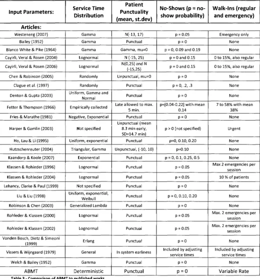
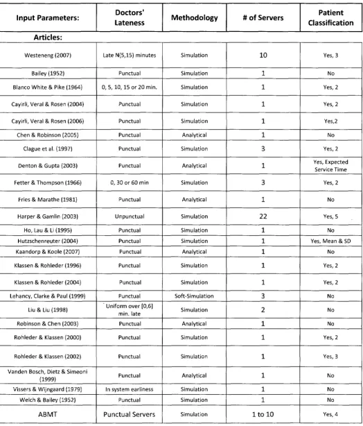
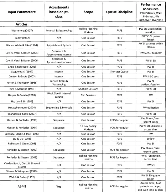
Building on Westeneng's work Table 3 (split onto 3 separate pages) combines Westeneng's key
parameters and cited works with that of this thesis. This combined table also compares the work of the
thesis (labelled as ABMT) with that of other published articles.
Input Parameters: Service Time Distribution
Patient Punctuality (mean, st.dev)
No-Shows (p = no-show probability) Walk-Ins (regular and emergency) Articles: Westeneng (2007) Bailey (1952) Blanco White & Pike (1964) Cayirli, Veral & Rosen (2004) Cayirli, Veral & Rosen (2006) Chen & Robinson (2005)
Clagueetal. (1997) Denton & Gupta (2003) Fetter & Thompson (1966)
Fries & Marathe (1981) Harper SGamlin (2003)
Ho, Lau & Li (1995) Hutzschenreuter (2004) Kaandorp & Koole (2007) Klassen & Rohleder (1996) Klassen & Rohleder (2004) Lehancy, Clarke & Paul (1999)
Liu & Liu (1998) Robinson & Chen (2003) Rohleder & Klassen (2000)
Rohleder & Klassen (2002) Vanden Bosch, Dietz & Simeoni
(1999)
Vissers & Wijngaard (1979) Welch & Bailey (1952)
ABMT Gamma Gamma Gamma Lognormal Lognormal Randomly Randomly Uniform, Gamma and
Normal Empirically collected Negative, Exponential Not specified Uniform, exponential Triangular, Gamma Exponential Lognormal Lognormal Not specified Uniform, exponential, Weibull Generalized Lambda Lognormal Lognormal Erlang General Gamma Deterministic N(-13, 17) Punctual Gamma, mu=0
N (-15, 25) N(0,25)andN
(-15,25) Unpunctual, mu=0
Punctual Punctual Late allowed to max.
5 min. Punctual Unpunctual (mean
8.3 min early, SD=14.7 min) Punctual Unpunctual, (-10,10) Punctual Punctual Punctual Punctual Punctual Punctual Punctual Punctual Punctual In system earliness
Punctual
Punctual
p = 0.05 p = 0 p = 0,0.09 and 0.19
p = 0and0.15 p = 0and0.15
p = 0 p = 0, .2, .3
p = 0
p=[0.04-0.22] with mean 0.14
p = 0 p > 0 (not specified)
p=0, 0.10, 0.20 p=0.10 p = 0, 0.1, 0.25, 0.5
p = 0.05 p = 0.05 p = 0 p = 0, 0.10, 0.20
p = 0 p = 0.05
p = 0.05
p = 0 Included by adjusting
service times p = 0
p = 0
Emergency only None None Oto 15%, also regular Oto 15%, also regular
None None None 7 to 58% with mean
38% None Urgent None None None Max 2 emergencies per
session 10 % of patients
None None None
Max. 2 emergencies per session Max. 2 emergencies per
session None Included by adjusting
service times None
Input Parameters: Doctors'
Lateness Methodology # of Servers
Patient Classification
Articles:
Westeneng (2007)
Bailey (1952) Blanco White & Pike (1964)
Cayirli, Veral & Rosen (2004) Cayirli, Veral & Rosen (2006) Chen & Robinson (2005)
Clagueetal. (1997) Denton & Gupta (2003)
Fetter & Thompson (1966) Fries & Marathe (1981)
Harper &Gamlin (2003) Ho, Lau & Li (1995) Hutzschenreuter (2004) Kaandorp & Koole (2007) Klassen & Rohleder (1996)
Klassen & Rohleder (2004) Lehancy, Clarke & Paul (1999)
Liu & Liu (1998) Robinson & Chen (2003) Rohleder & Klassen (2000)
Rohleder & Klassen (2002) Vanden Bosch, Dietz & Simeoni
(1999)
Vissers & Wijngaard (1979) Welch & Bailey (1952)
ABMT
Late N{5,15) minutes
Punctual 0, 5, 10,15 or 20 min.
Punctual Punctual Punctual Punctual Punctual 0,30 or 60 min
Punctual Un punctual Punctual Punctual Punctual Punctual Punctual Punctual Uniform over [0,6]
min. late Punctual Punctual
Punctual
Punctual In system earliness
Punctual Punctual Servers Simulation Simulation Simulation Simulation Simulation Analytical Simulation Analytical Simulation Analytical Simulation Simulation Simulation Analytical Simulation Simulation Soft-Simulation Simulation Analytical Simulation Simulation Analytical Simulation Simulation Simulation 10 1 1 1 1 1 3 1 3 1 22 1 1 1 1 1 3 2 1 1 1 1 1 1
l t o l O
Yes, 3 No Yes, 2 Yes, 2 Yes,2 No Yes, 2 Yes, Expected Service Time Yes, 2 No Yes, 5 No Yes, Mean&SD No Yes, 2 Yes, 2 No No No Yes, 2 Yes, 3 No No No Yes, 4
Table 3 Continued - Comparison of ABMT to published works
Input Parameters:
Adjustments based on pt.
class
Scope Queue Discipline
Performance Measures
PW=Patients_Wait SI=Server_ldle SO=Server O v e r t i m e
Articles:
W e s t e n e n g (2007)
Bailey (1952)
Blanco W h i t e & Pike (1964)
Cayirli, Veral & Rosen (2004)
Cayirli, Veral & Rosen (2006)
Chen & Robinson (2005) C l a g u e e t a l . (1997) Denton & Gupta (2003)
Fetter & T h o m p s o n (1966)
Fries & M a r a t h e (1981)
Harper S G a m l i n (2003)
Ho, Lau & Li (1995)
Hutzschenreuter (2004)
Kaandorp & Koole (2007)
K l a s s e n & R o h l e d e r ( 1 9 9 6 )
Klassen & Rohleder (2004)
Lehancy, Clarke & Paul (1999) Liu & Liu (1998) Robinson & Chen (2003)
Rohleder & Klassen (2000)
Rohleder & Klassen (2002)
Vanden Bosch, Dietz & Simeoni (1999)
Vissers & W i j n g a a r d (1979)
W e l c h & Bailey (1952)
ABMT
Interval & Sequencing
N/A
A p p o i n t m e n t System
Sequence & A p p o i n t m e n t Interval
Sequence & A p p o i n t m e n t Interval
N/A
Interval Interval Service Times &
Sequencing IN/A Block Size & Interval
Length N/A
Sequencing & Intervals
N/A Sequence Sequence N/A IN/A N/A Sequence Sequence N/A N/A N/A Yes Rolling Planning Horizon One Session One Session One Session One Session One Session One Session One Session One Session
M u l t i p l e Sessions
Ten Sessions
One Session
One Session
One Session
One Session
10 Day Rolling Horizon One Session One Session One Session One Session Rolling Planning Horizon One Session One Session One Session Rolling Planning Horizon FAFS FCFS FCFS FCFS FAFS FAFS Shortest Queue FCFS FCFS FCFS FCFS FCFS FCFS FCFS
FCFS f o r regular
FCFS f o r regular
FCFS FCFS FCFS
FCFS f o r Regular
FCFS f o r Regular
FCFS
FCFS
FCFS
FCFS f o r regular
PW SO SI utilization, w o r k l o a d PW SO SI queue
length PW SI patients w i t h i n
30 min
PW SO SI,'fairness'
PW SI SO
P W S I P W S I PW SI SO cost
P W S I patients/session
PW SI SO
PW
P W S I
PW utilization
PW SI SO PW SI m i n . / m a x .
urgent cases PW SI SO utilization
access t i m e
PW
SI f l o w PWSI PW SI m i n . / m a x .
urgent cases PW SI utilization,
access t i m e
P W S O
P W S I PW SI SO q u e u e
length Access Time, % o f patients o n t a r g e t , avg. w a i t t i m e by class
2.4 Literature Review Conclusions
The literature review has established:
That simulation is an acceptable means by which to create a decision support system, especially
in those cases where the system is complex and has many stakeholders.
The pros and cons of simulation and where it is most applicable
That simulation in healthcare is a widely accepted practice and has the capability to yield
positive verifiable and validated results.
That agent-based simulation is appropriate for the level of abstraction required to model a
diagnostic imaging scheduling system.
That outpatient scheduling has been studied via simulation before but not through agent-based
modelling.
That when modelling outpatient scheduling there are a standard set of parameters that must be
considered.
That there is no established standard decision support tool for the scheduling of diagnostic
imaging services.
It is based on these facts that we chose to build a decision support tool using agent-based
simulation to assess the impact of operational level changes to a diagnostic imaging scheduling system.
3. Agent-Based Modelling Tool (ABMT)
This chapter describes the Agent-Based Modelling Tool (ABMT) built using NetLogo™ a programmable
modelling environment well suited to complex dynamic systems. In 3.1 we introduce the ABMT
Environment and in 3.2 the Patients. In 3.3 we describe the Scheduling Discipline. We end the chapter
with a presentation of the User Interface.
3,1 ABMT Environment
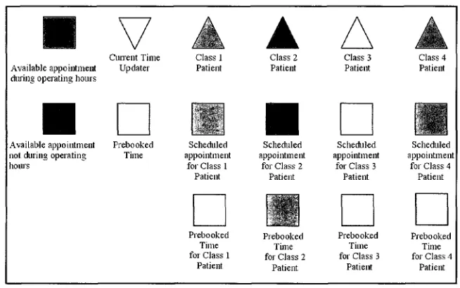
NetLogo™ uses two different types of agents, 'patches' and 'turtles'. Patches are stationary and
the collection of patches form the environment in which the turtles exist and move. In Figure 3 we see
the agents used in the ABMT. Squares are patches and triangles are turtles. The colours green, blue,
yellow and brown represent the different patient priority classes. Red, black and grey represent times
that are not currently or cannot be used for scheduling a patient.
Current Time Available appointment Updater during operating hours
Available appointment not Airing operating hours
Prebooked Time
Class 1 Patient
Scheduled appointment
for Class 1 Patient
Prebooked Time for Class 1
Patient
Class 2 Patient
Scheduled appointment
for Class 2 Patient
Prebooked Time for Class 2
Patient
Class 3 Patient
Scheduled appointment
for Class 3 Patient
Prebooked Time for Class 3
Patient
Class 4 Patient
Scheduled appointment
for Class 4 Patient
Prebooked Time for Class 4
Patient
Figure 3 - Patches and Turtle
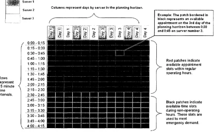
The planning horizon is composed entirely of patches arranged to form a grid (See Figure 4).
When configured for a single server each column represents a single day and each row a specific time of
day. The number of days in the horizon is adjustable, but the number of appointment blocks in a day
(red and black combined) is not. At current there are 96 blocks (patches) per day (column), each
representing a 15 minute time block. Red patches are appointments that are available for scheduling
and black patches are periods when patients cannot be booked. The number of operating hours per day
Columns represent days in the planning horizon. Rows represent 15 minute time intervals. 0:00 0:15-0:30 0:30-0:45 0:45 -1:00 1:00-1:15 1:15-1:30 1:30-1:45 1:45-2:00 . 2 : 0 0 . ^ 1 5 2:15-2:30
2:30 - 2:45 2 : 4 5 - 3 :
3:00-3:15 3:15-3:30 3:30 3:45 4:00-3:45 4:00 4:15
Example: The patch bordered in black represents an available appointment on the 9th day of the planning horizon between 0:30 and 0:45.
Red patches indicate available appointment slots within regular operating hours.
Black patches indicate available time slots during non-operating hours. These slots are used to meet emergency demand.
Figure 4 - Layout of Simulation Environment
For multi-server scenarios each column represents a specific server on a specific day. Figure 5 depicts a multi-server scenario with 3 servers and 2.5 hours of scheduled time per day.
Server 1 Servei 2 Server 3 f
.m
;Rows represent 15 minute time intervals. QiPJL: 0:15 - 0:30- 0:451:00 - 1:151:30 - 1:45-2:00 • 2:15-.2:30..: 2:45- 3:00-3:15-Columns represent days by server in the planning horizon.
V
3:30 3:45 4:00 -3:45 -4:00 -4:15Example: The patch bordered in black represents an available appointment on the 3rd day of the planning horrizon between 0:30 and 0:45 on server number 3.
Red patches indicate available appointment slots within regular operating hours.
Black patches indicate available time slots during non-operating hours. These slots are used to meet emergency demand.
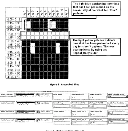
Prebooked times are appointment slots set aside from the standard first come first serve
scheduling process. These prebooked times are used in many cases to meet demand for patients who
cannot wait for diagnostic imaging services. For example, many patients admitted to the hospital
require service from the diagnostic imaging department during their stay. It is inefficient and hazardous
to force them to wait for an appointment like a non-admitted patient might. To that end appointments
are set aside each day to meet the potential demand for diagnostic imaging services from admitted
patients. Figure 6 depicts an example of a planning horizon with prebooked time. Figure 7 shows 4 of
the prebooked time controls.
The Ii(jht blue patches indicate time that has been prebooked on the second clay of the week for class 2 patients.
Figure 6 - Prebooked Time
i f o f f W M WV - P ' e b o o k e d
Day of the week 1
Pre booked Ti me
^ O f f R ePM t- t > a i l v _ l
l i — _ ~ — . . 1 ! Servers_Booked 1
1* 1
Weekly _Prebook_Stan2 . 5
Week 1 y _Pre b o ok _Fjid
• r •s
Weekly _Prebooked_l_CliS5
||Class2 ~~y\
T g l i Weekly_Prebooked_2
Day oF lhe week 2 i ^ g n Repeat _Daily_2 i Serve rs_Booked_2
j | l |
Weekly _Prebook_ Start _2 i
3 . 2 5
1 Weekly _Prebcok_B<l_2
j 3 . 2 5
iWeekly Prebooked 2 Class
|.CUss2 v |
' T g " Weekly _Prebooked_3
Day_oF_the_week_3 1 f p g r i Repeat _Daily_3 1 Servers _ Bo oked_3
u
[weekly_Prebook_Start_3
3 . 7 5
Weekly_Pmbook_&id J3
3 . 7 5
(Weekly _Prebooked_3_C lass
jfciass 2 v j
JT?g£ Weekly _Prebooked_4
D-*y_oFjhe_week_4 3 I ^ O f f R ePe a t-Dairy_4 Servers Booked 4
;i'
i
] Weekly_Prebook_Start_4
. 5 . 7 5
! Weekly _Prebook_Btd_4
l| 1 1 5 . 7 5
Weekly _Prebo oked_4_CI ass
I^KT ZZZZZ3
3.2 Patients
Requests for patient service, also known simply as patients, are the driving force of the ABMT.
The following subsections describe the different types of patients, the method with which they come to
be in the system, and their interactions with each other and the simulation environment.
Patients, represented by turtles, come in 4 priority classes. These four classes are
representations of the patient priority class 1 through 4 used in Canadian hospitals; each patient
requesting service from the diagnostic imaging department is assigned a prior level by their physician.
Class 1 patients require immediate attention while class 2, 3 and 4 patients are to be scheduled if
possible within 2,10 and 28 days respectively based on ministry of health guidelines.
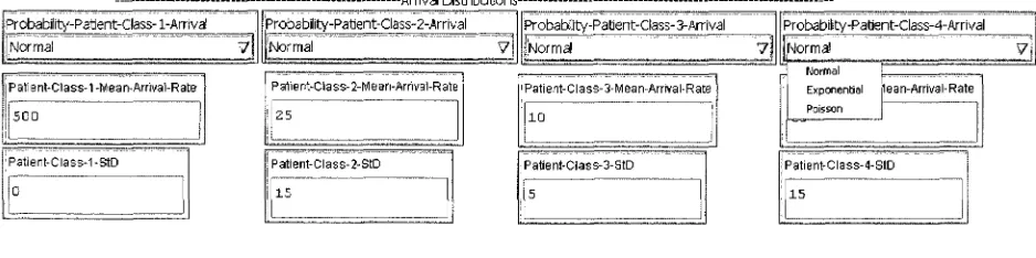
Requests for patient service are received or 'arrive' according to probability distributions. The
distributions govern the inter-arrival time between patients of the same class. The distributions
available in NetLogo™ to describe the arrival rate are normal, exponential and Poisson. The user selects
the distribution that most accurately describes their system from a drop down menu as seen below.
Seen below in Figure 8 are the controls for the arrival rates of all 4 patient priority classes, example
means and standard deviations can be seen in the input boxes. In this example we can see that Class 1
patients have a mean interarrival time of 500 minutes, thus Class 1 patients' arrivals are normally
distributed with a mean of 500 minutes.
Arrival Distributions Probability-Patlent-Class-l-Arrival
Normal V
Patient-Class-1 -Mean- Arrival-Rate
JSOD
I
Patient-Class-1-StD 0
ProbabIity-Parjent-Class-2-Arrival
f o r m a l V]
Patient-Class- 2-Mean-Arrival-R at | 25
Patient-Class- 2-StD I S
I :—: 1
probability-Parjent-Class-3-Arrival
Normal 7 j
Patient-Class-3-Mean-Arrival-Rate 10
Patient-Class-3-StD 5
Probability-Paflent-Class-4-Arrival
[Normal V j
Exponential flean-Arrival-Rate
Poisson
Patient-Class-4-StD
15
Figure 8 - Arrival Distribution Control
The ABMT uses a deterministic service time of 15 minutes per patient. The assumption is made
that all scans can be completed within 15 minutes and subsequent scans do not begin until 15 minutes
has elapsed since the preceding scan started. This may not always be the reality but because the focus
of this study is on access time not wait time and the resulting difference is considered negligible. In
prebooked for 'None.' That is to say that one of the patches, representing 15 minutes, is made
unavailable for scheduling to account for the time lost to the 30 minute appointment.
3.3 Scheduling Discipline
Scheduling operates on a first come first serve basis with the exception of emergency patients
and prebooked time. After a patient arrives in the system based on an arrival rate, the scheduling
operation searches for an available appointment slot (red patch or appropriate prebooked time) by
moving the patient down its current column patch by patch. If a patch is booked (not red or the
appropriate prebooked time colour) the patient moves on to the next patch (the one directly below it).
This continues until one of two things happens; if the patient comes to the end of scheduled time for a
day it is moved to the top of the next column (next day) and it continues its search or alternatively if the
patient finds an available appointment its search stops. Once the patient finds an available appointment
it changes the colour of the free appointment patch to its patient priority class colour (blue patients
make blue patches, brown patients make brown patches etc.). In this way patients are assigned to
appointment slots. When scheduling reaches the end of the planning horizon it resumes at the
beginning. This process is depicted below in Figure 9.
CO CO
Q Q 0:00-0:15
0:15-0:30 0:36-0:45 0:45-1:00 1:00-1:15 i:15-1:30
1:30-1:45 1:45-2:00
00
Da
y o>
Da
y
2:00- 2:15-2:30 2:45 3:00 3:153:30 - 3:45-
4:00-2:15] 2:30 2:45 3:00 3:15 3:30 3:45 4:00 -4:15
c
T— > v ro Q <N >* ro Q CO >, ro Q T >. ro Q in > s ro Q CD >. ro Q I-->> ro Q CO >. ro Q a> >> ro o o T— >-ro uV " 1
T— ;
>. ! (U ! a i 0:00 0:15 6:30 0:45 1j00 1:15 1:30-1:45 1:45-2:00 0:15 •0:30 0:45 1:00 1:15 •7:30 2:00-2:15 2:15-2:30 2:30 - 2:45 2:45 - 3:00 3:00-3:15 "3:15"-3730
3:30 - 3:45 3:45-4:00
4:00-4:15
Example: Pictured above and adjacent is an example of patient scheduling for a single server. Section A shows the route the patient will take in search of an appointment (I then II then III). Section B shows us that it is a class 4 patient, as indicated by the brown triangle. Section C shows us t h e final result of the search and t h e subsequent appointment.
Figure 9 Continued - Scheduling Process: Single Server
Scheduling of patients occurs in much t h e same way f o r multiple servers as it does f o r a single server.
The primary difference is that t h e scheduling operation attempts t o schedule patients on each server at
the earliest possible time before moving on t o a later time. Figure 10 depicts scheduling in a multi-server
scenario.
«^"fc J P " I , -P"% .^™E - S ~ k ^3~V J P ^ I S % ^ 3 " u ^~K .*^"fc ^ S - l
O Cl O Cl Q O O O O Q O O
0:00 - 0:15 ^ M ^ j j ^ B E ^ B W I B E W B P
0:15-0:30 i B B M E f f ^ * ^ w f I M W
0:30 - 0:450:45 - 1:00 f ^ f | p p j 1:00- 1:15
1:15-1:30 1:30-1:45 1:45-2:00
2:00-2:15 H
2:15-2.30 B O M
2:30-2:45 fiBl
2:45-3:00 • • ]
3:00-3:15 • • !
3:15-3:30 0 f l |
3:30-3:45 0 1 9 1
3:45-4:00 • H !
4:00-4:15 • • !
Example: Pictured adjacent is an example of patient scheduling in a multi-server scenario. In this case there are 3 servers and the planning horizon is 4 days long. The scheduling operation begins searching for an available appointment slot at the beginning of day 2 on the first server (furthest to the left in the horizon). This appointment is booked so the search continues by considering the availability of the 2n server during that same period. The 2n server is also unavailable so the search continues with the 3r server. Because this server is also unavailable and there are no more servers the search begins again in the next time period (0:15 - 0:30) with the Is server. The search continues in this way until an available appointment is found.
Figure 10 - Scheduling Process: Multi-Server
Class 1 patients require immediate attention; they pre-empt other patients, bumping them from
their currently scheduled slot to the subsequent appointment slot. Bumping is the only action that takes
precedence over prebooked time and the only action that can result in overtime for the hospital staff.
The bumping process can be seen below in Figure 11. After the bump, all patients are moved forward in
the same day. So, while the patient waits more time for service while in the clinic, it does not affect wait
time as defined.
1 r—
>. to D C\l ->. ro a co >. ro Q •sfr >-. ra Q U) •>. ro Q CO
• > .
ro Q r^ ->, ro Q CO
> • .
ro a a> >> ro Q o T — ^ S ro a ,_ | -*— i >.: ro > " I 1:00 1:15 1:30 1:45 [ 2:00 I 2:15 2:30-2:45 3:00 3:15 3:30 3:45 4:00 1:15 1:30 1:45 2:00 2:15 2 : 3 0 ! 2:45 i 3:00 I 3:15 3:30 3:45 4:00 4:15 0:00-0:15 0:15-0:30 0 : ^ 0 ^ : 4 5 0:45 - 1^00 1:00-1:15 1:15-1:30 1:30-1:45 1:45-2:00 ~2:00-2:15 2:15 - 2:30 2:30 - 2:45 2:45 - 3:00 3:00-3:15 3:15-3:30 3:30-3:45 3:45_- 4:00 "4:00-4:15
Figure 11 - Bumping: Before and After
The simulator works by scheduling patients in future appointment slots relative to a constantly
updated 'current time'. Because the simulator uses a static number of days in its planning horizon it is
necessary to reuse days (columns) to prevent the horizon from becoming full. Once scheduling reaches
the end of the horizon (the far right column) it continues at the beginning of the horizon (the far left
column).
Beginning from the first appointment slot on the first day of the horizon the current time
'updater' moves from appointment slot to subsequent appointment slot on each tick of the system.
When the updater moves to an appointment it clears the patch of any previous appointments, returning
the patch to its original (unscheduled) colour (red, black, or grey). In this way appointment slots are
cleared for future appointments allowing for a stable queue of scheduled appointments to be simulated
indefinitely. Additionally, the updater is used in the scheduling process to determine where the
scheduling operation should begin its search for appointments. For example, patients are never
3.4 User Interface
3.4.1 Setup & Go
These controls update the main display area with the currently inputted prebooked times and initiate
the simulation. Setup also clears the graphical outputs of the model as well as the average wait times
and percentage of patients who exceed guidelines.
3.4.2 Data Recording
NetLogo™ allows the user to export data from simulations to external files. The ABMT has been
configured to export the patient class and wait time data for each patient that is scheduled to a
Microsoft Excel file. The GUI controls allow the user to choose whether or not they wish to record data,
delete existing data or close the file the data is being recorded to.
3.4.3 Random Fill
The ABMT was designed to assist hospital decision makers in assessing changes to scheduling in
diagnostic imaging systems. In order to accurately capture the current state of an existing system it is
necessary to also simulate the existing queue of patients. The random fill functionality fills the planning
horizon with class 4 patients up to a specified number of days. For example, if the user wished to model
a system that at present has a 4 week wait time they would select a random fill of 28 days so that
scheduling of patients would begin on the 29th day.
3.4.4 Simulation Run Time
The 'Days_to_run' input controls the duration of the simulation. The user enters the number of
simulated days they wish the model to run for and the ABMT halts operation after that number of
simulated days have passed.
3.4.5 Number of Servers
This control allows the user to select the number of servers that will be used in the system.
3.4.6 Scheduled Hours per Day
This input determines the division between available appointments during operating hours (red patches)
and available appoints during non-operating hours (black patches).
3.4.7 Information Display
The simulator's graphical user interface has been designed to give the user as much relevant data as
possible regarding the progress of a simulated model. At present there are several output figures,
graphics and charts to help the user make an initial analysis of the model being simulated.