Abstract
Thompson, Denis Brian. FINDING HOMOLOGOUS GENES WITH PRIMERS DESIGNED USING EVOLUTIONARY MODELS. (Under the direction of Henry Schaffer.)
FINDING HOMOLOGOUS GENES WITH PRIMERS DESIGNED USING EVOLUTIONARY MODELS
by
DENIS BRIAN THOMPSON
A dissertation
submitted to the Graduate Faculty of North Carolina State University
in partial fulfillment of the requirements for the degree of Doctor of Philosophy
BIOMATHEMATICS
Raleigh 2003
APPROVED BY
Henry Schaffer, Chair of Advisory Committee
Michael Purugganan
Charlie Eugene Smith
Personal Biography
Acknowledgments
I want to express my appreciation to a few people who helped me bring this dissertation to completion, and who enriched my life during graduate school.
An important part of my life in the last 3 years has been the delightful companionship I’ve shared with Laurie. I am deeply grateful to Laurie for being on my side, for giving me smart and truly helpful advice, and for giving me caring support. All these gifts have had a positive effect on my grad school experience and on other aspects of my life. But mainly all the time we’ve spent together means a lot to me.
To my dear family I want to say how much I appreciate your love and support. I appreciate y’all most of all for being there and for being yourselves throughout this grad school process. One relatively small but noteworthy part of all this support was the C++, Igor, and other computer help, including eleventh hour debugging help, I received from my dear brothers.
I thank Jeff Thorne for generously meeting with me some in Summer 2001, and from January 2002 until the completion of this project. The final form of the science of this dissertation is based largely on Jeff’s vision. (I did all the research in this dissertation after January 2001.)
I am deeply grateful to Henry Schaffer for noticing in May 2001 (when he attended my seminar) that I was floundering, and for going out of his way to e-mail me, offer help, and then make some phone calls to arrange help for me. Other people must have seen or known I was in trouble, but no one else reached out.
energy in my education, and for believing in me.
I also want to thank Henry for some of the most productive and educational discussions about the actual content of Biomathematics I have had in school. These interactions have been what graduate school is supposed to consist of.
This dissertation would not have happened without Jeff and Henry.
A smart person recently told me that the community of fellow students is most educational part of school. For me a big contributor in this respect was Doug Robinson. Doug was a gigantic help during the months I worked on this version of my project. He let me look at his code so I could figure out some algorithms, and let me copy chunks of 3 or 4 of his codon-handling functions. He directed me to the C++ TCL matrix objects. He gave me invaluable help in late September 2003 when I thought I had a bug in my code and needed to figure it out within 24 hours. And he answered e-mail questions from me at other times. Doug also generously explained several issues about evolutionary models, and other bioinformatics concepts. Doug amazingly always responded to my questions and requests in an upbeat and positive way. I can’t thank Doug enough for all these particular pieces of help, and in general for being someone I could ask “dumb” questions of.
I want to express my appreciation for some of the precious friends I have had outside of school during graduate school. I treasure my wonderful friendship with Carol. And I am likewise glad for and thankful for many dear friends who have made my life richer and more rewarding in these past few years: Val, Sam, Paul, Leslie, Amy, Marcia, Samantha, Penny (and thanks for the rides into campus in spring 2002), Elise, Harlan, and Corey. Also thanks to Bob, Elisabeth, Jane, Lisa, and Carmen.
role as Director of Graduate Studies; Jim Selgrade for his help in committee reassignments; and Jackie Dietz for suggestions about statistical tests. I thank Terry Byron for being helpful and really caring about stat and biomath students’ work environments and computer
resources. And thanks to Ann Ethridge for caring about my welfare all along, and for inducing me to take action to improve my situation in December 2001.
A few friends have especially enriched my life around school in these grad school years. These people made my time in the computer lab, in the grad student offices, in class, and also away from school, more fun and connected and real: Russell, Dan, Sarah, Teri, Liz, Jason, Cindy, Brian, Marta, and Virginia. These friends have meant a great deal to me. (Russell showing up out of the blue a few days before my defense is perhaps the happiest surprise I’ve ever had.)
Finally, I’m glad for Irene’s timely questions, for her getting me to think, and for her helping me get work done near the last months of the project. But mostly I appreciate her caring about me.
With much appreciation,
Table of Contents
page . . . . x List of Tables
xii List of Figures . . . .
xv List of Symbols and Abbreviations . . .
1 Introduction . . . .
Chapter 1
Example of contemporary primer design process . . . 1 4 The standard primer design method . . .
9 Definition of the problem to be addressed . . .
10 Weaknesses of the standard method . . .
15 Improving one aspect of primer design —prediction . . . .
17 Algorithms and programs for primer design . . .
24 Evolutionary model based prediction of new sequences
—derivation of equations . . .
30 Derivation of the performance measure for site-by-site
prediction method . . .
38 A mathematical model of the standard primer design method
43 Further justification of using a probability distribution to
represent the standard primer design method . . . .
44 Comparing prediction methods . . .
47 Comparing sets of these values with the
Wilcoxon-Nemenyi-McDonald-Thompson two-sided all-treatments multiple
comparison procedure . . . .
50 Other ways of comparing performance measures . . . .
Chapter 2
57 Comparison of evolutionary model based prediction methods
and standard method —relative performance at predicting a single related amino acid sequence . . .
57 Descriptions of the three alignments used in this study . . .
64 Breaking the alignments into segments, and results of the
statistical test . . .
68 Comparison of the standard primer design method and the
single site evolutionary model based method. . .
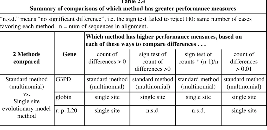
73 Summary of comparing differences between performance
measures between standard method (multinomial) and single site evolutionary model method . . .
74 Multiple-site information . . . .
77 A multisite evolutionary model based method . . .
81 Does the size of the segments affect results? . . .
83 Comparison of the multisite evolutionary model based method
and the standard primer design method . . .
87 Summary of comparing differences between performance
measures between multisite evolutionary model method and standard method . . . .
89 Comparison of the multisite evolutionary model based method
and the single site evolutionary model based method . . . .
93 Summary of comparing differences between performance
measures between multisite evolutionary model method and single site evolutionary model method . . .
95 Correlation of P(LO_seq|LI_set)’s within a segment . . . .
Chapter 3 Using Information in Clusters . . . . 98 99 Description of the prediction algorithm that makes use of
cluster information . . . .
100 Results of comparing three prediction methods . . . .
104 Comparison of the prediction methods on trees of different
average evolutionary distances . . .
106 Interpretation of Figures . . . .
Chapter 4 Comparison of pool construction methods . . . . 111
113 Detailed description of the all-degenerate-primer pool
construction method . . . .
114 Detailed description of the “whole tree” pool construction
method . . . .
116 Detailed description of the “one subpool per attachment
point” pool construction method . . .
117 Results . . . .
126 Does pool size affect the “fraction of pool with few
mismatches” performance measure? . . . .
132 Conclusions from this research . . .
Chapter 5
136 Directions for future research . . . .
139 . . .
References
142 Derivation of model to predict related sequences given the
List of Tables
page 1 Bassett et al used sequences from these proteins to design
primers . . . Table 1.1
2 Conserved segments used by Bassett et al . . .
Table 1.2
3 Bassett et al’s upstream primer pool . . . .
Table 1.3
4 Bassett et al’s downstream primer pool . . . .
Table 1.4
Length of PCR primers used in various research . . . 5 Table 1.5
11 Segments with low degeneracy are uncommon . . . .
Table 1.6
23 Number of citations of primer-design software . . .
Table 1.7
Number of citations of primer-design methods papers . . . . 23 Table 1.8
41 Comparison of multinomial and modified multinomial . . .
Table 1.9
65 Results of Wilcoxon-Nemenyi-McDonald-Thompson tests
on the G3PD alignment data . . . Table 2.1
66 Results of Wilcoxon-Nemenyi-McDonald-Thompson tests on
the alpha globin and beta globin alignment data . . . Table 2.2
67 Results of Wilcoxon-Nemenyi-McDonald-Thompson tests
on the ribosomal protein L20 alignment data . . . Table 2.3
74 Summary of comparisons of which method has greater
performance measures . . . Table 2.4
88 Summary of comparisons: Which method has greater
performance measures? . . . Table 2.5
94 Summary of comparisons of which method has greater
performance measures . . . Table 2.6
98 Average Pairwise Percent Identities of sequences within each
101 Average percent identities of each prediction method
Table 3.2
103 Cluster method comparisons Results of
Wilcoxon-Nemenyi-McDonald-Thompson tests on the G3PD alignment data . . Table 3.3
105 aa APPI for each tree . . . .
List of Figures
page 26 Hypothetical Trees . . . .
Figure 1.1
27 Attachment Points . . .
Figure 1.2
47 Histogram of Probabilities . . .
Figure 1.3
48 Differences of average
†
P LO_seq LI_set
(
)
’s are not normally distributed . . . Figure 1.451 Log scale histogram of a set of differences . . . .
Figure 1.5
59 A subset of the Goldman group’s G3PD phylogenetic tree
Figure 2.1
62 Phylogenetic tree showing relation of amino acid sequences in
concatenated alpha globin and beth globin alignment . . . . Figure 2.2
63 The phylogenetic tree of the 11 sequence ribosomal protein
L20 alignment used in the analysis . . . Figure 2.3
70 Comparison of standard prediction method and evolutionary
single-site prediction method for G3PD alignment . . . . Figure 2.4
71 Comparison of performance measures for the two prediction
methods, on the alpha globin and beta globin alignments . . Figure 2.5
73 Log-scale histogram of differences in probabilities . . . . .
Figure 2.6
82 Comparison of analyses done on different segment lengths
Figure 2.7
83 Log-scale histogram of differences in probabilities —G3PD
alignment . . . Figure 2.8
85 Log-scale histogram of differences in probabilities —globin
alignments . . . . Figure 2.9
87 Log-scale histogram of differences in probabilities
—ribosomal protein L20 alignment . . . Figure 2.10
89 Log-scale histogram of differences in probabilities —G3PD
alignment . . . Figure 2.11
91 Log-scale histogram of differences in probabilities —globin
93 Log-scale histogram of differences in probabilities
—ribosomal protein L20 alignment . . . Figure 2.13
96 Location, in alpha and beta globin alignments, of sequences
for which the single site evolutionary model method predicted significantly better than the multinomial method predicted Figure 2.14
97 Location, in r. p. L20 alignment, of segments for which the
single site performance measure predicted significantly better than the multinomial method . . . . Figure 2.15
102 Percent identities are not normally distributed . . . .
Figure 3.1
107 Relative performance of three prediction methods on
alignments with different APPI’s —segments of length 28 aa’s . . . Figure 3.2
108 Relative performance of three prediction methods on
alignments with different APPI’s —segments of length 20 aa’s . . . Figure 3.3
109 Relative performance of three prediction methods on
alignments with different APPI’s —segments of length 14 aa’s . . . Figure 3.4
110 Relative performance of three prediction methods on
alignments with different APPI’s —segments of length 7 aa’s . . . Figure 3.5
118 alpha and beta globin phylogenetic tree with codon
branchlengths . . . Figure 4.1
118 Comparison of 3 pool construction methods on the alpha
globin alignment . . . Figure 4.2
119 alpha globin pool performance measure vs pool size, for the
three pool construction methods . . . Figure 4.3
121 Comparison of three pool construction methods . . .
Figure 4.4
122 Three histograms for the beta globin data . . .
Figure 4.5
123 Newick representation of the G3PD tree with branch lengths
in units of expected nucleotide substitutions per codon . . . Figure 4.6
124 G3PD pool performance measures vs. APPI . . .
125 3 Histograms of “pool fraction” performance measure for
G3PD data . . . Figure 4.8
125 Newick representation of the phylogenetic tree for the
ribosomal protein L20 alignment . . . Figure 4.9
128 Pool fraction vs. Pool size, for alpha globin gene . . .
Figure 4.10
129 Influence of pool size on performance in beta globin . . .
Figure 4.11
130 Pool size and performance, G3PD data . . .
Figure 4.12
131 Pool size and performance, ribosomal protein L50 data . .
List of Symbols and Abbreviations
Equation Eq.
nucleotide nt
complementary DNA cDNA
Polymerase chain reaction PCR
ribosomal protein L20 rp L20
left-in set of sequences LI_set
left-out sequence LO_seq
average pairwise percent identity APPI
G3PD Glyceraldehyde 3 phosphate dehydrogenase Amino Acid
AA or aa
Right-hand side of an equation RHS
LHS Left-hand side of an equation Meaning Symbol or
Chapter 1
Example of contemporary primer design process
Basset et al. (2002) wanted to find the gene for the ethylene receptor, ETR1, in the peach, Prunus persica. The ethylene receptor gene had previously been found and sequenced in several species. (See Table 1.1.) Basset et al. predicted that the peach sequence would be similar to the known sequences for this gene in the other species. So to learn the exact sequence in the peach, Basset et al. followed a process familiar to experimental biologists: they designed PCR primers (oligonucleotides) that would bind to DNA sequences coding for parts of the known ethylene receptor amino acid (aa) sequences, used the primers in a PCR reaction with peach genomic DNA, cloned the fragment amplified in the reaction, and
screened a peach cDNA library for sequences complementary to the cloned fragment. Using this method they successfully found the sequence of the peach ETR1 gene.
They designed these PCR primers using an alignment of seven known amino acid sequences —sequences of proteins known to bind to ethylene. The proteins in the alignment they used are listed in Table 1.1.
1. ethylene responsive factor from rice
2. putative ethylene receptor from the carnation 3. ethylene response sensor from Arabidopsis 4. ethylene receptor from Arabidopsis
5. putative ethylene receptor from the tomato 6. ETR1 homolog from the tomato
7. ethylene response sensor from Rumex palustris (common name "Marsh Dock")
Table 1.1
Bassett et al. used sequences of these proteins to design primers
The parts of the alignment of the known protein sequences that Bassett et al. designed PCR primers to hybridize to the nucleotide sequence for. In this figure, the six aa’s in the
upstream site are separated from neighboring sequences on each side with a space, as are the seven aa’s in the downstream primer site. These spaces do not indicate a gap in the
sequences. “ERS” means “ethylene response sensor.” ETR1 means “ethylene receptor.”
protein
Table 1.2
Conserved segments used by Basset et al.
downstream primer site upstream primer site
DFLA VMNHEMR TPMH
DFLA VMNHEMR TPMH
DFLA VMNHEMR SAMH
DFLA VMNHEMR TPMH
DFLA VMNHEMR TPMH
EFLS VMNHEMR TPIH
DFLA VMNHEMR TPMN
LM LVHIIP DLL
LM LVHIIP DLL
LM LVHIIP DLL
LM LVHIIP DLL
LM LVHIIP DLL
LW LVYIIP DLL
LM LVHIIP DLL
Rumex ERS1 tomato ETR1 tomato ERS Arabidopsis ETR1 Arabidopsis ERS carnation ERS rice ERS
In the downstream segment there is 100% identity between the seven known aa sequences. In the upstream segment the carnation sequence is different from the other aa sequences at one of the six aa sites; otherwise there is 100% identity between the seven sequences here.
Pool of “degenerate primers”
So, for example, if there were a sequence of 3 aa’s, and there were two codons in the genetic code for each of the 3 aa’s in this sequence, then the “completely degenerate” primer pool would contain oligonucleotides of 2 x 2 x 2 = 8 different sequences.
The reason to have completely degenerate set of primers in the pool is to make the primers able to amplify the sequence in a related species, even if different species code for the aa sequence using different codons. (The assumption is that the related species will have the same aa sequence, but perhaps not the same nucleotide sequence.) Different species might code for a particular aa at a particular site with different codons because the species have different codon preferences, or just because of chance.
The primers Basset et al. designed, shown in Tables 1.3 and 1.4, do not contain every possible codon that might code for the corresponding amino acids. But in most cases they do. See the row labeled “Fraction of codons coding for this aa represented in primer pool” in Figures 1.3 and 1.4.
The molecules present in the primer pool are shown on the sense row. Nucleotides within parentheses are the different degenerate sequences. In the nucleotide sequence, “I”
indicates inosine, a synthetic nucleotide that when incorporated into DNA will pair with any of the four natural nucleotides (Watanabe et al. 2001, Bartl 1997). See comments in text on guanine residues at 5’ and 3’ ends.
Table 1.3
Basset et al.’s upstream primer pool
1 of 4 3 of 3
3 of 3 2 of 2
4 of 4 4 of 6
fraction of codons for this aa
represented in primer pool P I I H V L
aa 1-letter symbol:
aa 3-letter symbol Leu Val His Ile Ile Pro
-3’ G CCT AT(A/C/T) AT(A/C/T) CA(C/T) GTI CTI G
sense:
known aa sequences, in the position corresponding to this guanine, are tryptophan (W) and methionine (M). Each of these aa’s is coded for by one codon. And both of those codons end in a G. So the guanine would bind to every nucleotide sequence seen in the given alignment.
(It is unclear why Basset et al. include a guanine (G) residue at the 3’ end of their upstream primer. The amino acid residues, in the known aa sequences, in the position corresponding the the guanine at the 3’ end, are threonine and serine. No codon coding for either of these aa’s begins with a G.)
The set of molecules in the primer pool (i.e. that are included in the PCR reaction mixture) are shown on the antisense row. The sequence of codons translated into aa’s is shown on the sense row. In the nucleotide sequence, “I” indicates inosine. (The rightmost two nucleotides in the primer, “TC” in the antisense strand, will bind with two of the 6 codons for serine, in addition to binding to the two codons for arginine. Only arginine, R, appears in the corresponding site in the known aa sequenes. See Table 1.1.)
Table 1.4
Basset et al.’s downstream primer pool
2 of 2 2 of 2
1 of 2 2 of 2
4 of 4 1 of 1 1 of 1
fraction of codons for this aa represented in primer pool
R M E H N M V
aa 1-letter symbol:
aa 3-letter symbol Val Met Asn His Glu Met Arg
AG ATG GA(G/A) CAT AA(T/C) ATG GTx
sense: 5’- -3’
-5’ TC TAC CT(C/T) GTA TT(A/G) TAC CAI antisense:
3’-The standard primer design method
have about 50% GC (guanine:cytosine) content. Rarely can such primers be designed.” I will refer to this method as the “standard” primer design method, because it is widely used.
Optimum length of primers
Sells and Chernoff do not cite any science proving that 18 to 24 nucleotides (the length corresponding to six to eight aa’s) is the optimum length for a PCR primer. Nor do they even give their reason for advocating this length. But this length is used by many researchers. Table 1.5 shows a small sample of papers that used PCR to screen for genes related to a
known alignment of genes, and the lengths of primer used.
These PCR primers were all used to screen for related genes.
Table 1.5
Length of PCR primers used in various research
Length of corresponding peptide
Length of primers, in nucleotides Paper
7 aa’s 9 aa’s 7, 8 aa’s
8 aa’s 10, 11 aa’s
6 aa’s 7, 8 aa’s
20, 21 25 21, 24 23, 24 29, 33
18 20
Wünschiers et al. 2001 Venugopal et al. 2002 Oshima et al. 2002 Kirimura et al. 1999 Jones et al. 1995 Chen et al. 1998 Basset et al. 2002
Although Sells and Chernoff do not list them, there are easily discernible design constraints that make “too short” primers undesirable, and other design constraints that make “too long” primers undesirable.
the researcher is interested in. Löffert et al. (1997), in a methods paper about PCR primers, discourage the use of primers of length 15 nucleotides or shorter for this reason.
Longer primers are more difficult to design because longer stretches of highly-conserved sequence are more rare than short stretches of highly-conserved sequence. Using a longer primer also makes it more likely that the sequence of interest will have evolved into a different sequence in the species the researcher is attempting to find the gene in.
Longer primers are also undesirable because, if one is using a pool of primers representing all degenerate sequences coding for an aa sequence, then the longer the primer, the smaller the concentration (in the PCR reaction) of the primer with the correct sequence. For example, suppose a researcher wants to probe for an amino acid sequence that is 7 amino acids long. And suppose that 3 of these aa’s are each coded for by 4 codons, and the remaining four aa’s are each coded for by 2 codons. Then the completely degenerate primer pool would contain representatives of
†
43⋅24 =1024 different oligonucleotide sequences. Compare that 7 aa long primer pool with the pool for a sequence 11 aa’s long, 5 aa’s of which are each coded for by 4 codons, and six aa’s of which are each coded for by 2 codons. In this second case the completely degenerate primer pool would contain representatives of
†
45
⋅26
=65,536 different oligonucleotide sequences.
The researchers listed in Table 1.5, and Sells and Chernoff, have decided that 18 to 24 nucleotides is the approximate optimum range. Bartl (1997) in a methods paper essentially agrees. She advocates using primers of a length 18 to 30 nucleotides. But her methods paper is about using inosines to allow one to construct longer primers that will bind to many
degenerate sequences, but do not contain so many different-sequence primers, so do not have to be so dilute.
Sells and Chernoff advocate the use of degenerate primers for the reasons discussed above in the section titled “Pool of degenerate primers.”
Sells and Chernoff advocate finding low degeneracy primers so the correct primer will not be too diluted. Bassett et al. designed for low degeneracy when they chose the site for their downstream primer to be an aa sequence containing two methionine residues among the seven aa’s. Only one codon codes for methionine. Making a pool of primers “completely
degenerate” for a methionine at one site results in multiplying the number of different-sequence primers in the pool by a factor of one.
GC Content
Sells and Chernoff write that 50% GC content is desirable because that content gives the primer-target DNA hybrid a predictable melting temperature. This characteristic is not necessary for success of amplification. Times and temperatures of the PCR reaction can be adjusted so the reaction is successful for different primer-target DNA melting temperatures.
Optimizing all the design desiderata
After describing their ideal primers, Sells and Chernoff note that “rarely can such primers be designed.” They make this statement because it can be difficult to simultaneously optimize the design requirements they list, while also optimizing other design requirements of PCR primers. (Other design requirements are discussed below.) For example, the alignment of known genes might not contain a completely invariant stretch of seven amino acids. Or the only invariant stretch might contain a high proportion of amino acids coded for by 4 or 6 codons each, making the pool of degenerate primers not meet their degeneracy requirement. (The aa’s Ser, Leu, Pro, Arg, Thr, Val, Ala, and Gly are each coded for by four or six codons.)
that “there are no infallible rules to guide the final selection.”
The number of sequences in the given set
Usually when designing primers to screen for related genes, researchers use an alignment of several sequences to design the primers. One example of this method is the Basset et al. example presented above. Other examples are: Wünschiers et al. (2001) used several prokaryotic sequences to design primers to find Fe-hydrogenase in a green alga; Venugopal et al. (2002) used “all available fish growth hormone protein sequences” to identify a
conserved region and design a primer to bind to it, to find the gene in carp; Jones et al. (1995) designed primers based on an alignment of sequences from eight species.
Other researchers have used just two genes to identify conserved regions and design their primers to find related genes. For example Kirimura et al. (1999) used two sequences —one from a lily and one from a yeast— to design a primer to find a gene in the fungus Aspergillus niger.
The number of species the “new” sequence is sought in
In the examples given so far, the researchers’ goal was to find the gene in one particular species. Sometimes the researcher has the aim of finding a gene in multiple species. For example Gould et al. (1989) used one set of PCR primers to find the succinate
dehydrogenase (SDH) gene in humans, mice, rats, Xenopus, Drosophila, Arabidopsis, two species of yeast, and Dictyostelium. The primers were designed based on conserved
sequences identified by comparing the SDH amino acid sequence in just two species: E. coli and bovine.
not have to chemically screen for gene sequences in these species. As time goes on,
researchers will have less need to chemically screen for genes in commonly studied species. As more complete genomes become available, researchers will be more able to simply search sequence databases.
But there will still be the need for chemical screening because, of course, some researchers study species for which the genomes are not available online. For example Kevin Moulton screened for genes in multiple non-Drosophila fly species. (Kevin Moulton, 2002, personal communication.)
Definition of the Problem to be addressed
The problem stated as given-find
Above are examples and descriptions of the primer design problem. Here is a more precise expression of the primer design problem this dissertation addresses:
Given: a set of n aligned, related, protein-coding sequences (either nucleotide, aa, or codon) of length k.
Find: the one sequence, out of all possible sequences, that is “most likely” to be the sequence of a new member of the set (“new” defined just below).
The Basset et al. example above is an example of an experimentalist solving this problem.
Meaning of terms in given-find statement
By a “new member of the set” I simply mean another sequence related to the given
sequences, that is not yet considered to be a member of the set. So the sequence is new to the set in question. “New” does not indicate the sequence is newly evolved. Rather, the
The new sequence is the sequence that is sought experimentally with the PCR reactions. The probability that is used to judge which sequence is “most likely” is not adjusted based on whether the gene is sought with PCR or another laboratory screening procedure.
This dissertation addresses this problem only in protein-coding sequences. Calculations are done in the amino acid realm in Chapters 2 and 3, and in the codon realm in Chapter 4.
I will sometimes refer to the given set of sequences as the “known” sequences.
Further specification of the problem
I think of each sequence in the known set as belonging to a different species, although the methods presented here would probably be valid to apply to duplicated genes within the same species. (This dissertation does not attempt to apply the methods presented here to the
problem of screening for related genes within one species.) I also think of the unknown or new sequence as being in yet another species. I will sometimes refer to a sequence as “the sequence of a known species” —the “known species” (singular) being one of the species to which the known sequences belong.
I will address these questions in unrooted trees, so the conclusions will be helpful to experimentalists. Often an experimentalist will have a set of sequences, but not have easy access to a rooted topology for the species. He might not have a rooted topology because he does not have easy access to an outgroup sequence.
Requires segments with low degeneracy and other characteristics
One weakness of the standard primer design method is that it requires the presence, in the alignment of interest, of segments with high identity and low degeneracy. (“Degeneracy” here means the product of the number of codons in the genetic code, for the most-prevalent aa at each site in the segment.) If such segments are not present in the known alignment, or are not present at suitable locations within the alignment, then the researcher would want to have an alternative primer design method. (Currently, a researcher faced with this problem would do the best he could with the given sequences. Sells and Chernoff even write that the ideal part of an alignment is often difficult to find. Sells and Chernoff list a precise cutoff value for degeneracy, but not for percent identity.) This dissertation aims to demonstrate a primer design method suitable for use in segments that might not meet the Sells and Chernoff
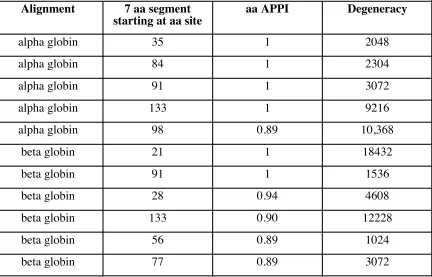
The degeneracies were calculated based on one most-frequent aa at each site. “aa APPI” is average pairwise percent identity on the amino acid level.
Table 1.6
Segments with low degeneracy are uncommon
12228 0.90 133 beta globin 3072 0.89 77 1024 0.89 56 beta globin 4608 28 0.94 18432 1536 1 1 91 21 2048 2304 3072 9216 10,368 0.89 98 1 133 1 91 1 84 1 35 beta globin beta globin beta globin beta globin alpha globin alpha globin alpha globin alpha globin alpha globin Degeneracy aa APPI
criteria.
Sometimes the set of aa’s in an aligned segment happen to be of too-high degeneracy to allow the construction of a pool of primers that contains every combination of degenerate codons at each site. For example, Table 1.6 shows the degeneracies and average pairwise percent identities for selected segments of the alpha globin and beta globin alignments. The table shows 11 seven-aa segments (out of the 40 total seven-aa segments of the two genes) with high identities. One can see from Figure 1.6 that only one of these eleven most-conserved segments of the two genes is of low enough degeneracy to fit the Sells and Chernoff criterion for degeneracy: the segment from aa sites 56 to 62 in the beta globin gene.
There are other criteria a researcher must worry about. One must find two appropriate sites an appropriate distance apart, for the upstream and downstream primers of the PCR reaction.
An alternate method for constructing a pool of primers, that would not constrain the
researcher’s choice of segment within alignment, as much as the standard method, would be useful.
Lack of success with standard method
A primer design method that has a higher success rate than the contemporary primer design method would also be welcomed by researchers. (By “success” I mean the designed
primers amplify the gene of interest in the new species.) Primers designed via the Sells and Chernoff method do not always amplify the gene of interest. That fact is not surprising —no experimental technique works all the time.
based on anecdotes such as the ones described in the next section, it happens a significant fraction of the time.
Examples of not finding genes
Here I note a couple of examples of the standard primer design method not working, just to give a sense of how the method works in the lab.
The work of Basset et al. (2002) demonstrates that “Sells and Chernoff” designed primers do not always amplify the target gene. The two primer pools shown in Figures 1.3 and 1.4 (of this dissertation) were the primers that did successfully amplify. But Bassett and her coworkers report that they made several (at least 6) upstream and downstream primer pools designed to bind to different short stretches of the sequence. They tried them in PCR
reactions in various combinations —thus empirically determining which amplified from the target DNA better, worse, or not at all.
Basset et al.’s work shows one way researchers deal with this lack of guaranteed success: by empirically trying multiple primers designed to bind to different stretches of the aa sequence. Sells and Chernoff (1995) suggest this approach. My goal in this dissertation is to invent an improved primer design method that will decrease the amount of this extra experimental effort that is necessary.
Another example of lack of success in finding related genes with PCR was related to me by Michael Purugganan. He was searching for MADS-box transcription factor genes in Clarkia species and mosses. He designed primers based on an alignment of approximately 20 genes, but was not able to amplify the desired gene from his species of interest. (Michael
Purugganan, personal communication, June 2003.)
Chernoff method, in which the primers failed to amplify the desired product from fly species. (J. Kevin Moulton, 2002, personal communication.)
Reasons to think evolutionary model based prediction method might work better
In the standard method, each sequence in the known alignment is given the same weight in “predicting” the new sequence. That is, in most cases researchers do not take into account if one species in the alignment is relatively closely related to the “new” species of interest, (if they are looking in just one species) and give that sequence more weight than the other sequences. Nor do researchers usually consider if the set of known sequences is biased toward part of the evolutionary tree. For example, perhaps the gene of interest has been studied in several species of insects, and just one or two species each of fish, mammals, and shellfish. In this case a researcher might have an alignment of 15 known sequences of this gene, where half of these known sequences are from insects. If this researcher wants to screen for the gene in a species of mammal, it might make sense for him to give special consideration to the 2 known mammal sequences in the known alignment. From my discussions with researchers, this kind of special consideration is not usually done.
There are reasonable reasons why researchers following the standard method don’t usually give extra weight to closely related species: following the Sells and Chernoff method, if one finds a region of 100% identity, relative distance does not matter. Also, if the researcher is interested in finding the gene in multiple new species, and wants to screen with one pool of primers, identifying the closely related known species might not make sense.
But a natural way to take into account biased representation of species is to use the
Improving one aspect of primer design —prediction
This dissertation does not attempt to offer improvements to all aspects and stages of primer design, of which there are many. Nor do I present a comprehensive algorithm for primer design. (I refer the reader to Bartl 1997, and Sells and Chernoff 1995 for such an algorithm.) I present algorithms intended to improve on one aspect of primer design: the prediction of the target sequence.
The following aspects of primer design are important to think about when designing a primer: • The amplified product must be of an appropriate size. Bartl (1997) advises her
readers to choose a distance between the upstream and downstream primers of 200 to 2000 bases. Shorter primers can be difficult to see on the post-PCR gel, and difficult to purify from it. Fragments longer that 2000 bp might not amplify, without special considerations about the duration of the extension step in the PCR reaction.
• If a PCR primer that is designed based on related sequences is used to amplify from the genomic DNA of the target species, unknown introns in the target species can cause problems two ways. First, an intron within the short stretch of nucleotides that a primer is designed to bind to would probably impede primer binding to target DNA. Second, an unknown intron between the two PCR
primers could either inhibit successful amplification, or would make the amplified fragment to be of an unexpected size, perhaps causing the researcher to overlook it.
that contains 1000 different varieties (particular sequences) of oligonucleotides. In this case there will likely be many varieties of the primer that form hairpins, and many that do not.
• If, in the target genome, there are many copies of a short DNA sequence that a primer will bind to, the primer might be competitively bound by those other sites, thus interfering with amplification from the site in the gene of interest
(Donehower et al., 1990. p. 34). Mitsuhashi (1996a,b) presented a method for attempting to circumvent this problem during primer design. But his method works only for single primers, not pools of primers.
• Many researchers consider the 3’ end of the primer to be especially important in priming, and therefore apply different requirements to these nucleotides than to other nucleotides in the primer. Löffert et al. (1997) urge their readers to avoid a run of 3 or more C or G residues, and to use a special buffer in the PCR reaction so as to diminish the problem of mis-pairing at the 3’ end. Kevin Moulton tried to make the 3’-most aa in his primer region be a methionine or tryptophan, each of which is coded for in the genetic code by just one codon. (Kevin Moulton, 2002, personal communication.)
• Primers of different lengths and different sequences will have different optimum PCR reaction conditions. So primer design is interrelated with the design of particular PCR reaction conditions, such as: temperatures of the melting, annealing, and extension steps; duration of each step; buffer; salts; and proofreading or non-proofreading polymerase.
Focus of this dissertation
Methods are relevant to non-PCR screening
One can screen a DNA library for the presence of a particular sequence using either hybridization of a long nucleic acid probe, or PCR. (Ausubel et al. 2002. p. 6-1) Both methods make use of DNA’s property of hybridization between complementary DNA
strands, to chemically find the sequence of interest. The methods are similar in that one must have a predicted sequence (in the form of a molecule) to find the desired sequence.
The methods presented in this dissertation could, with some modification, be used to design long nucleic acid probes, in addition to PCR primers. But herein I will always describe the methods in terms of PCR primers.
Algorithms and programs for primer design
Over the years, researchers have developed a number of computer programs to assist with some aspect of designing PCR primers to screen for related genes. Although none of these programs directly solve the problem that is the focus of this dissertation —prediction of sequences in related genes— they solve similar or related problems and deserve attention.
Programs that assist in choosing a primer site
An early program is Montpetit et al.’s (1992) OLIGOSCAN. This program helped researchers choose a primer site by searching through a set of DNA sequences, for occurrences of partial or complete identity between the sequences and a proposed oligonucleotide sequence.
in a set of sequences. Their program suggests the best primer for binding to (and therefore detecting the presence of) a sequence common to groups of species. For example, given a set of hantavirus genomes, the program could find sequences common to all of the genomes. Such a sequence could be used as the target of a diagnostic PCR, to determine if a patient is infected with a hantavirus. This program could, alternatively, be used to find short regions of high homology in an alignment.
One set of programs that advanced the automated design of PCR primers able to bind to aligned sequences was Gibbs et al.’s (1998) GPRIME package. (This package of programs could also be used to help design probes in non-PCR hybridization-based screening
methods.) The program scans a set of aligned DNA (not aa) sequences, identifying short stretches of low variability between the sequences in the alignment. This program could be used to quickly identify appropriate primer sites in a DNA alignment.
This program is flexible in that it works on both protein coding and non-protein-coding regions of a DNA sequence. The program apparently does not distinguish between these two types of regions though. So it always identifies variability on the DNA level. It can not take into account possible codon structure of a DNA sequence. Therefore a weakness of the program is that it can not identify a part of an alignment that codes for identical aa sequences with different nucleotide sequences.
Mitsuhashi program takes into account that there are two classes of sequences the oligonucleotide might bind to: 1. the intended target sequence that is the length of the oligonucleotide and 2. other DNA sequences present as “background” in the PCR reaction. (The program allows the user to specify a database of background sequences.) The program calculates how strongly the oligo will bind to each of these two DNA sequences. It tells the user which oligonucleotides have a better ratio of high affinity for their target sequence and low affinity for background sequences.
The program also will inform the user of issues that might interfere with amplification in a PCR reaction: hairpin structures; primer-primer interactions; and GC content of sub-regions of an oligonucleotide, such as the 3’ end.
Mitsuhashi’s program could be used in some creative ways to decrease problems stemming from primer-primer binding within pools of PCR primers. But the program’s intended purpose is to help design effective PCR primers given a single target DNA sequence, not an alignment of aa sequences.
A program with an alternative primer design algorithm
oligo corresponds to the highly conserved aa’s, the 5’ end of each oligo is designed by the second scheme.
Consider the twelve 3’-most nucleotides of the oligos that constitute the pool. These sequences of these twelve nucleotides include all combinations of codons coding for the four highly conserved amino acids.
The sequence of the remaining 18 nucleotides, on the 5’ ends of these oligos (corresponding to the remaining 6 amino acids) is a single (non-degenerate) sequence consisting of the most probable nucleotide predicted for each position. The CODEHOP algorithm sets these most-probable nucleotides to be simply the most common codon (according to a codon usage table specified by the user) coding for the most common aa at that position in the aa sequence.
(Sometimes Rose et al. would include all degenerate oligos coding for just three amino acids on the end, not four.)
Rose et al. choose this strategy because the 3’ end is widely considered to be more important for primer success in PCR than other parts of the primer are (Löffert et al. 1997; Kevin Moulton, 2002, personal communication). A primer pool designed using Rose et al.’s algorithm will be certain to contain oligos that are an exact match for the 3’ part of the target species’ nucleotide sequence, assuming the amino acid sequence is completely conserved in the target species. And those “3’ exact match” oligos will be present in a higher
concentration than “3’ exact match” oligos in a pool designed by the Sells and Chernoff method, because the 5’ end is not degenerate in the Rose method.
Efficacy of the CODEHOP method
tests they successfully amplified genes of the gene family of interest. And the CODEHOP method has been successfully used by researchers since then (see Figure 1.?? below).
Efficacy of CODEHOP relative to the standard method
Rose et al. wanted to demonstrate their strategy’s efficacy relative to the standard method of designing primers for screening for related genes. To this end, their compare their results, from one of the three tests in their paper, with results reported by other researchers in two previous papers. The two previous papers reported the use of primers designed against the same short segment (within an alignment of reverse transcriptase genes) that Rose et al. design primers to.
Rose’s work compares favorably with these previous reports. For example Wichman and Van Der Bussche (1992) use their primers to amplify reverse transcriptase from human genomic DNA, and found two unique sequences related to reverse transcriptase. But Rose et al. found 24 unique sequences related to reverse transcriptase, when they used the
CODEHOP primers with human genomic DNA.
It is unfortunate, though, that Rose et al. did not do direct comparisons between the
CODEHOP and standard primers. Direct comparisons would have allowed one to draw more definitive conclusions.
A direct comparison would have been to use primers designed by the standard method in PCR reactions that were otherwise identical to the PCR reactions Rose’s primers were used in. Instead of that direct comparison, Rose et al. compared their results in their experiments with results reported in the previous papers. Rose et al. designed their primers to the same particular segments within the reverse transcriptase alignment, as the two previous papers. But besides that consistency between Rose et al.’s experiments, and the other two
primer designs were based on; how the target DNA was purified; how dilute the target DNA was in the reaction; the genome the target DNA was from; reaction conditions; the number of different pools of primers tested in the search for the one that worked best; how clones were selected from the finished reaction; and others. (Rose et al. 1998, Donehower et al. 1990, Wichman et al. 1992.)
Rose et al. claim that their CODEHOP primers were able to amplify related genes that were “too diverged from known sequences to be readily isolated by standard methods.” But they never compared their CODEHOP primers to primers designed by the standard method, in experiments where other reaction conditions were held constant.
Another issue, that confuses exactly what is being compared between the Rose paper and the other two, is that in both of the papers that Rose uses to represent the standard method, the primers contained “extra”, non-degenerate nucleotides on the 5’ end, containing a restriction site for cloning. Those extra nucleotides make the primers that are supposed to represent the standard method similar, in one way, to CODEHOPE-designed primers.
How often researchers use these programs
Out of all these programs (algorithms) to assist in primer design, the most widely used is Rose et al.’s CODEHOP, as judged by the number of times the papers have been cited. Table 1.7 lists the number of times each paper announcing one of the algorithms above has been cited, between its publication date and June, 2003.
Table 1.8 shows the number of times two primer design methods papers were cited. This table shows that many researchers use the primer-design method Sells and Chernoff describe in their 1995 paper, without citing that paper. For example, all the papers listed in Table 1.1, above, use essentially the Sells and Chernoff method, yet none of them cite Sells and
consider the primer design strategy Cells and Chernoff describe to be “common
knowledge”. Sells and Chernoff did not invent the method; they described an already widely used method. So researchers probably do not feel the need to cite a reference when they use it.
Evolutionary methods
85 Rose et al. (1998)
Each paper listed here describes an algorithm, and announces a program implementing that algorithm, for designing PCR primers, for uses similar to or equivalent to the problem this dissertation addresses. The number of citations is for the time between the paper’s publication date and June 2003, according to the ISI® “Science Citation Index Expanded.”
5 11 11 10
Number of Citations Paper
5 Gibbs et al. (1998)
Mitsuhashi (1996b) Mitsuhashi (1996a)
Dopazo and Sobrino (1993) Montpetit et al. (1992)
Table 1.7
Number of citations of primer-design software
The number of citations is for the time between the paper’s publication date and June 2003, according to the ISI® “Science Citation Index Expanded.”(The Bartl reference is a chapter in a book and so is not in the database.)
Number of Citations Paper
N.A. Bartl (1997)
1 Sells and Chernoff (1995)
Table 1.8
No research in the literature has attempted to use evolutionary models to predict sequences in related species, or to use those predictions to design PCR primers for screening.
Evolutionary model based prediction of new sequences —derivation of equations
The problem of designing primers (or other probes) to screen for related sequences can be stated as:
Given:
a set of n aligned, related, protein-coding sequences (either nucleotide, aa, or codon) of length k.
Find:
the one sequence, out of all possible sequences, that is “most likely”, according to stated assumptions and a model, to be the sequence of a generalized new member of the set.
The section “Definition of the problem to be addressed”, above, which first stated the
problem as given-find, discusses a few aspects of the problem, including the meaning of the phrase “new member of the set”.
The word “generalized”, and other terminology
This version of the given-find statement is a little different from the statement in the section above, in that this statement uses the concept of a “generalized” new sequence (a
“generalized” new member of a set of sequences.)
Relative to a set of known sequences, a “generalized new sequence” is an unknown
I will refer to the species containing the generalized new sequence as the “generalized new species.” Considering a set of species, whose evolutionary relationships are known, a “generalized new species” is one whose evolutionary relationship to the given set is unknown (unspecified). One does not know how the species containing the sequence is related to the known species. One does not know which of the known species the new species is most closely related to.
From a given set of sequences one can infer a most likely phylogenetic tree, including branch lengths. I refer to this tree, which includes only the species in the known set, as the “known tree”. Sometimes I refer to this tree as “the inferred tree”, if there is little chance the reader will confuse the specified tree with a different inferred tree.
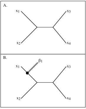
Figure 1.1 A. depicts a simple, hypothetical, known tree. If I learn a new sequence and its relation to the known sequences, I would show the relation to the known sequences by placing a new branch, terminating in a tip node, somewhere on the known tree. An example of such an attached branch is depicted in Figure 1.1 B. I refer to the point at which this new branch attaches to the known tree the “attachment point.” For a generalized new sequence, the attachment point and length of new branch are unknown.
A generalized new sequence is “general” in that one is not specifying where the branch and tip that would represent the new sequence are located on the known tree.
Equations involving generalized new sequences
In the context of these equations, the length and location of the attachment point that would connect the generalized new sequence’s branch to the known tree is, as stated above,
unknown. It is possible the appropriate attachment point might be any point on any branch of the known tree.
Because the attachment point is not known, it is not straightforward to calculate the
x
1x
2x
3x
4x
1x
2x
3x
4b1
A.
B.
Figure 1.1. Hypothetical trees. A) A known phylogenetic tree. B) The tree with “new” sequence
†
generalized species’ probabilities associated with the evolutionary model, as one would calculate these probabilities for known nodes of a tree.
The solution to this difficulty is to model generalized species’ probabilities as the average of what the probability would be if the attachment point were located in a finite set of positions on the tree (the finite set representing all possible attachment points on the tree.) An example, hypothetical, finite set of attachment points is depicted in Figure 1.2.
x
1x
2x
3x
4A
3A
2A
4A
5A
1Figure 1.2. Attachment points. The finite set of attachment points are designated A1 through A5. The
known sequences at the tips are indicated by
†
x1 to
†
x4.
The goal of the following derivation
To solve the given-find problem in the section above, I define a probability of a particular sequence being the generalized new sequence, given the data and the tree inferred from that data.
†
P
(
bgenX,q)
Here
†
nucleotides, amino acids, or codons.
†
bgen Œ
{
all sequences of length k}
†
X= the set of known sequencesx1 to xn, all of length k.
†
q = the parameters of the inferred tree
Parameters included in
†
q are the topology, branch lengths, and a priori probabilities of states of a root node. Theta does not include information about what internal node of the tree is ancestral to any other internal node. The parameter
†
q will be omitted from the equations, for the sake of notational simplicity.
Let the place where a new branch attaches to the known tree be attachment point A.
†
AΠthe set of attachment points
One could imagine, of course, a new branch attaching at any “point” on a branch of the known tree. But in this dissertation I use the term “attachment point” to refer to a finite set of points. There is one of these “attachment points” at the midpoint of each branch of the tree. Below, I calculate a weighted average over this discrete set of points (a graphical example of which is in Figure 1.2) instead of an average over all possible points on all branches of the tree.
The variable a (alpha) represents the state (the sequence) of the node that is attachment point A.
†
a Œ
{
sequences of length k}
The variable B designates a tip node at the end of the attached branch. The state at node B is
†
b (beta), where
†
In the equation
†
P
(
bgen X,q)
, the purpose of the “gen” subscript is to remind the reader that the attachment point (where the new branch joins the known tree) is not specified. If the attachment point is specified, this term would be:†
P
(
bAX,q,A)
This probability is: the probability of the particular sequence beta being the new sequence, given the known sequences X, the inferred tree
†
q, and that the new branch is attached at attachment point A.
The “A” subscript above is to remind the reader that the attachment point is specified.
(Both the “gen” subscript and the “A” subscript are superfluous, since the information they convey to the reader can be discerned from the list of “given” events, by noticing if the attachment point is present or absent in the list. I will sometimes leave off this subscript.)
The probability,
†
P
(
bgen X,q)
, is the number I want to calculate. To predict a most likely new sequence, one would calculate this probability for all possible sequences†
bgen and then choose the
†
bgen for which the probability is the maximum. My goal in the derivation below is to arrive at an equation: an expression for this probability as a function of the sequence data and the parameter
†
q .
Once I have this expression, I will be able to compute this probability, given the sequence data I start with, and use those numbers to design primers and pools of primers.
An aside on notation: events vs. sequences
In equations such as
†
P
(
bX,q)
, the variables†
b, X, and
†
are sets of outcomes of “experiments”, in the probability theory sense. So I am using the notation inconsistently when I define
†
b as a member of a set of sequences, and at the same time write the probability that the new sequence is
†
b as
†
P
(
bX,q)
. The two statements are inconsistent because I am on one hand saying†
b= sequence i
and on the other hand saying
†
b= "the outcome of experiment z is: sequence i"
To be perfectly consistent I would define
†
b to be a sequence and write that probability as
†
P
(
new=bX,q)
. But the language is easier in many cases if I am less strict. So I will often refer to†
b as a “sequence” while in the same section using expressions such as
†
P
(
bX,q)
and not
†
P
(
new=bX,q)
. The reader will always be able to tell what I mean based on context. If the context might not make the meaning completely clear to the reader, I will writeexpressions such as
†
P
(
new=bX)
or†
P
(
root=bX)
.The use of variable
†
b is just an example of this dissonance between an event —the outcome of an experiment being a particular state— and the state itself. All of the variables in the probability expressions have these dissonant meanings.
Derivation of the probability of interest
Here is a statement, simply Bayes’ rule, about a generalized new species.
†
P
(
bgen X,q)
=P
(
bgen,Xq)
P X(
q)
Eq. 1.1
The parameter
†
q does not affect the following derivation, so I will omit it from the equations in this section
†
P
(
bgen X)
=P
(
bgen,X)
P X( )
Eq. 1.2
The denominator of equation 1.2 is the whole-tree probability. Let lbe the state (sequence) of the root node. Given the structure of the tree:
†
P X
( )
= P X(
l)
P( )
l all possible lÂ
Eq 1.3
†
lŒ
{
sequences of length k}
.As mentioned above,
†
Consider the probability
†
P
(
bgen,X)
, which is the numerator of the RHS of equation 1.2. This probability equals a weighted average, over all attachment points on the tree†
P
(
bgen,X)
=[
P(
bA,X A)
P A( )
]
all AÂ
Eq. 1.4
where ‘A’ is an attachment point in the finite set of attachment points. And
†
bA is the state of
the tip at the end of the attached branch that is attached to the tree at attachment point ‘A’. For this version of the calculations I assume the attached branch is a constant length d.
Modeling attachment points
I am modeling the generalized ‘new’ species (meaning a species that is adding to a set of known species) as the average of the set of hypothetical species at the tips of branches which join the known tree at a finite set of attachment points. Exactly how those attachment points are distributed on the known tree will influence the results I get from this model.
constructed from other genes.
The distribution I use is one attachment point per branch, and weight the probability
associated with that attachment point proportionally to the length of the branch. This method models a uniform probability of where the new species appears on the known tree. So the probability
†
P A
( )
q in equation 1.4 is proportional to the length of the branch that attachment point A is on, relative to the branch lengths of all the branches. That is:†
P A
( )
=length of branch containing Alength of branch i all branches i
Â
Eq. 1.5 So the equation for our probability of interest is now
†
P
(
bgen X)
=P
(
bA,X A)
P A( )
[
]
all A
Â
P X
(
l)
P( )
l all possible lÂ
Eq. 1.6
Rewrite
†
P
(
bA,X A)
as a sum over all the possible states of the attachment point. (I set the root, in the model, to be at the current attachment point. So summing over the states of the attachment point is written, in equation 1.7 and below, as summing over the states of the root. The two statements are equivalent.)†
P
(
bgen X)
=P
(
bA,root =a,X A)
[
]
all a
Â
P A( )
È
Î
Í ˘
˚ ˙
all A
Â
P X
(
l)
P( )
l all possible lÂ
Where
†
a Œ
{
sequences of length k}
†
P
(
bgen X)
=P
(
bA root =a,X,A)
P root =(
a,X A)
[
]
all a
Â
P A( )
È Î Í ˘ ˚ ˙ all A
Â
P X
(
l)
P( )
l all possibleÂ
lEq. 1.8
The probability
†
P
(
bAroot =a,X,A)
is just the transition probability from the state†
a to the state
†
bA, for a branch of distance
†
d. This transition probability is not affected by the
structure of the tree, or by two of the given variables: the data X, and the particular attachment point A. So I can use the notation
†
ta Æb to represent this probability. This transition probability is for the distance
†
d, even though
†
d is not written.
Substituting in the transition probability notation, and rewriting the
†
P root =
(
a,X A)
term as†
P
(
Xroot =a,A)
P(
root =a A)
yields†
P
(
bgen X)
=ta ÆbP
(
Xa,A)
P(
a A)
[
]
all a
Â
P A( )
È Î Í ˘ ˚ ˙ all A
Â
P X
(
l)
P( )
l all possible lÂ
Eq. 1.9
The term
†
P
(
Xa,A)
is just the “likelihood” of the sequence†
a. In other words, it is the probability of the data, given that the sequence at attachment point (node) A is
†
a, considering the attachment point A to be ancestral to all other points in the tree (and given the topology of the tree,
†
Calculating probabilities using this formula
The goal of the derivation above was to arrive at a formula that, if I have in hand some sequence data X, allows me to calculate a value for
†
P
(
bgen X)
. Equation 1.9 meets that criterion.In the amino acid realm, I can calculate the RHS of equation 1.9, starting with amino acid alignment X, a phylogenetic tree inferred from the alignment (or known from other research on the represented species), and stationary probabilities of the amino acids known from Jones et al. (1992).
The instantaneous rate matrix for these amino acid models is calculated as follows. One starts with the entries in the PAM 1 matrix (except the matrix is transposed, so the transition is from the amino acid on row i to that on column j.) Each off-diagonal element is multiplied by
†
pj,
the stationary probability for amino acid j (from Jones et al. 1992) corresponding to the row j the element occupies. The on-diagonal element for each row is now calculated to be the opposite of the sum of the off-diagonal elements for that row. Next one calculates the linear combination that is the sum of all the on-diagonal elements, each multiplied by the
†
pj for the
row it occupies. Every on-diagonal and off-diagonal element is divided by this linear combination. The resultant matrix is the instantaneous rate matrix.
If I choose to work in the codon realm, I can calculate the RHS of equation 1.9 using the codon alignment X and a phylogenetic tree inferred from that alignment (or known from other research on the represented species).
For evolutionary models in the codon realm, I follow the methods of Yang (1997). The instantaneous rate matrix Q for these codon models is built using the codon stationary probabilities
†
p (
†
pj being the stationary probability for codon j) and Yang’s parameters
†