Enhancing dependence-based prefetching for better timeliness, coverage, and practicality

ABSTRACT

LIM, CHUNGSOO. Enhancing Dependence-based Prefetching for Better Timeliness,

Coverage, and Practicality. (Under the direction of Dr. Gregory T. Byrd).

This dissertation proposes an architecture that efficiently prefetches for loads whose effective addresses are dependent on previously-loaded values (dependence-based prefetching). For timely prefetches, the memory access patterns of producing loads are dynamically learned. These patterns (such as strides) are used to prefetch well ahead of the consumer load. Different prefetching algorithms are used for different patterns, and different algorithms are combined on top of dependence-based prefetching scheme. The proposed prefetcher is placed near the processor core and targets L1 cache misses, because removing L1 cache misses has greater performance potential than removing L2 cache misses.

For higher coverage, dependence-based prefetching is extended by augmenting the dependence relation identification mechanism, to include not only direct relations (y = x) but also linear relations (y = ax + b) between producer (x) and consumer (y) loads. With these additional relations, higher performance, measured in instructions per cycle (IPC), can be obtained.

Enhancing Dependence-based Prefetching for Better

Timeliness, Coverage, and Practicality

by

Chungsoo Lim

A dissertation submitted to the Graduate Faculty of

North Carolina State University

In partial fulfillment of the

Requirements for the degree of

Doctor of Philosophy

Computer Engineering

Raleigh, North Carolina

2009

APPROVED BY:

_______________________________ ______________________________

Dr. Gregory T. Byrd

Dr. Vincent W. Freeh

Chair of Advisory Committee

BIOGRAPHY

ACKNOWLEDGEMENTS

TABLE OF CONTENTS

LIST OF FIGURES... vi

LIST OF TABLES... viii

Chapter 1

Introduction………... 1

1.1

Motivation……….. 1

1.2

High level view of prefetching……….. 2

1.3

High level view of the proposed prefetching mechanism…………...……..….. 5

1.4

Contributions………. 7

Chapter 2

Related Work... 9

2.1

Alternatives to prefetching... 9

2.2

Hardware prefetching schemes... 11

2.3

Software prefetching schemes... 16

Chapter 3

Timely Dependence-based Prefetching... 18

3.1

Motivation... 18

3.2

Dependence-based prefetching mechanism – high level view... 20

3.3

Proposed dependence-based prefetching mechanism – high level view... 22

3.3.1

Key differences with existing mechanisms... 22

3.3.2

Jump pointer creation method... 24

3.3.3

Filtering mechanism... 27

3.4

Implementation... 28

3.4.1

Inserting into CT... 30

3.4.2

Updating CT... 31

3.4.3

Looking up CT... 33

3.4.4

An alternate CT structure……….. 35

3.5

Evaluation... 36

3.5.1

Experimental Setup... 36

3.5.2

Effectiveness of hardware-based JPT creation mechanism... 37

3.5.3

Jump pointer distance... 40

3.5.4

Jump pointer accuracy... 42

3.5.6

Sensitivity of the potential producer window to ports and access latency.. 47

3.5.7

Effectiveness of the proposed prefetcher... 49

3.6

Conclusion... 54

Chapter 4

Exploiting Linear Dependence Relations to Enhance Prefetching... 55

4.1

Motivation... 55

4.2

Linear relations... 56

4.3

Distributions of direct and linear relations... 58

4.4

Added hardware complexity... 60

4.4.1

Arithmetic units... 63

4.4.2

Dependence chain tracking logic... 63

4.4.3

Candidate pair table... 64

4.4.4

Data forwarding logic (direct-relation filtering mechanism)... 66

4.5

Evaluation... 67

4.5.1

Speedups... 67

4.5.2

Sensitivity to the size of the L2 cache………... 73

4.5.3

Sensitivity of the correlation table to ports and access latency………….. 77

4.5.4

Sensitivity of the potential producer window to ports and access latency.. 80

4.6

Conclusion... 82

Chapter 5

Using L2 Cache for Storing Prefetch Table... 84

5.1

Motivation... 84

5.2

Reconfigurable cache... 87

5.3

Implementing prefetch table in L2 cache... 88

5.4

Evaluation... 91

5.4.1

Impact of the L2 cache size on overall performance... 91

5.4.2

Performance with varying the partition size for JPT... 92

5.4.3

The effectiveness of the hash function... 98

5.5

Conclusion... 99

Chapter 6

Conclusion... 100

LIST OF FIGURES

Figure 3.1 Schematic of DBP... 21

Figure 3.2 Prefetching schemes for LDS... 25

Figure 3.3 Organization of the Proposed Prefetcher... 29

Figure 3.4 Example of Correlation Identification Unit... 31

Figure 3.5 Example of Jump Pointer Creation Unit and Jump Pointer Table... 33

Figure 3.6 Example of Correlation Table... 34

Figure 3.7 The effectiveness of JP creation mechanisms in terms of IPC... 40

Figure 3.8 Prefetch reference breakdown with varying jump pointer distance... 41

Figure 3.9

Influence of jump pointer distance on IPC... 42

Figure 3.10 Accuracy with varying jump distance... 44

Figure 3.11 Sensitiveness of the CT to the number of ports... 46

Figure 3.12 Sensitiveness of the CT to its access latency... 47

Figure 3.13 Sensitiveness of the PPW to the number of ports... 48

Figure 3.14 Sensitiveness of the PPW to its access latency... 49

Figure 3.15 Breakdown of prefetch hits: stride-based prefetch, jump pointer-based

prefetch, and chain-prefetch... 50

Figure 3.16 Performance comparison... 53

Figure 4.1 Code segments from mcf and bzip2... 57

Figure 4.2 Extra hardware for linear mechanisms... 62

Figure 4.3 Candidate pair table implementation... 66

Figure 4.4 Performance comparison with 1MB L2 cache... 71

Figure 4.5 Performance comparison with 2MB L2 cache... 71

Figure 4.6 Performance comparison with 4MB L2 cache... 72

Figure 4.7 Performance comparison with 8MB L2 cache... 72

Figure 4.8 Impact of the L2 cache size on the performance... 73

Figure 4.10 Performance improvements for bzip and art…... 76

Figure 4.11 Sensitiveness of the CT to the number of ports... 79

Figure 4.12 Sensitiveness of the CT to its access latency... 80

Figure 4.13 Sensitiveness of the PPW to the number of ports... 81

Figure 4.14 Sensitiveness of the PPW to its access latency... 82

Figure.5.1 Implementation of a reconfigurable cache... 88

Figure.5.2 Implementing a jump pointer table in the L2 cache... 89

Figure.5.3 The impact of the L2 cache size on overall performance... 92

Figure.5.4 Performance with varying the partition size for the jump pointer table in L2

caches: 1MB L2 Cache (top), 2MB L2 cache (middle), and 8MB (bottom) for

mcf... 95

Figure.5.5

Performance with varying the partition size for the jump pointer table in L2

caches: 1MB L2 Cache (top), 2MB L2 cache (middle), and 4MB L2 cache

for health... 97

LIST OF TABLES

Table 3.1 Simulation parameters... 37

Table 3.2 The number of jump pointers created for mcf and health... 39

Table 4.1 Frequency of occurrence (%) of dependence patterns... 59

Chapter 1

Introduction

1.1. Motivation

During the past decades, the gap between processor speed and memory speed widened, and this has been the most serious impediment to achieving higher performance. This phenomenon is due to trends in processor and memory designs. The trend in processor design is that processor clock period is reduced to achieve higher throughput, but the trend in memory design is in the direction of higher densities rather than in the direction of lower access latencies.

Due to this wide gap, current processors need more instruction-level parallelism to overcome the gap, but finding enough parallelism is not easy in most applications. Consequently, processors are likely to stay idle for many cycles, waiting for memory to provide requested data.

non-speculative techniques such as decoupled access/execute architecture [49], various cache designs [1, 8, 41, 54], and cache-conscious structure allocation [9, 10].

This dissertation focuses on prefetching mechanisms. There are three reasons for this. First, the potential of prefetching is very high, and none of the existing prefetching schemes is able to achieve the full potential. If prefetching can eliminate all cache misses, all load instructions can be considered as instructions that have execution latency of L1 cache hit latency. Second, prefetching doesn’t require a recovery procedure when a mis-prefetch occurs. Some performance degradation may occur, if a useful block is evicted by a prefetched block or if contention happens at the memory interface. However, this degradation can be minimized by giving priority to demand fetches over prefetches. Third, a prefetch mechanism can be easily combined with other techniques. For example, if prefetching is combined with value prediction [14], higher performance may be obtained. This is because value prediction is more effective for reducing dispatch-to-issue latency and prefetching can reduce issue-to-writeback latency. Prefetching makes value predictions validated earlier than the case without prefetching.

1.2. High level view of prefetching

schemes advocate using L2 cache, even though getting prefetched data from L2 cache takes time, because L2 cache doesn’t suffer cache pollution as much as L1 cache because of its big capacity. Also, a modern out-of-order pipeline may be able to hide L2 cache latency.

How to generate prefetch addresses can be further divided into two things: what to look at and what to look for in order to generate prefetch addresses.

Prefetching mechanisms rely on address streams. Streams can be either whole address streams from the processor, or miss address streams from L1 or L2 cache. By observing only miss address streams, some patterns cannot be discovered, but hardware complexity can be decreased and important patterns can still be observable. These streams can be localized by using program counter (PC) [33] or cache set numbers [16]. Localized stream may lead to finding new patterns and more efficient utilization of resources due to sharing.

Repeated pattern-based prefetching requires substantial amount of space and it takes time to learn repeated patterns, but it can cover more loads than stride-based prefetching.

One of more general prefetcher utilizing repeated pattern is distance prefetcher [22, 33]. Distance prefetching is a generalization of Markov prefetching [18]. Distance prefetching was originally designed for prefetching TLB entries, but the mechanism can be readily adapted to data prefetching. Distance prefetching uses the distance between two consecutive global miss addresses to index the correlation table. Each correlation table entry holds a list of deltas that have followed the entry’s delta in the past. One useful property of this prefetching scheme is that it can predict unseen addresses, because a sequence of delta can be shared by multiple address streams.

There are some mechanisms that have different ways of generating prefetch addresses. One such mechanism is dependence-based mechanism [43]. It identifies a set of producer instructions for a consumer load, and issues a prefetch request based on the value produced by the producer instructions. This mechanism is able to issue prefetches for almost all candidate loads, but may not be able to fully hide miss latencies.

Ideal prefetching eliminates all cache misses. In order to achieve this goal, a prefetch must be performed for every miss (coverage), each prefetched block should arrive at L1 cache or prefetch buffer before it is actually accessed by processor (timeliness), and every prefetched block has to be accessed by the processor (accuracy). In reality, these three requirements are hard to satisfy at the same time. If we want to increase coverage, more prefetches need to be issued. Among them, unnecessary prefetch requests exist inevitably, lowering accuracy. If we focus on timeliness, addresses of loads far away from the current instruction need to be predicted. This may decrease accuracy. If accuracy is the target, prefetches that have high probability of success are selectively issued, impairing coverage.

prefetches share resources, such as buses or cache, too much contention between the two may end up decreasing performance. This problem should be resolved to enjoy full potential of prefetching. Another practical problem is the implementation cost of prefetching. In order to achieve high coverage, accuracy, and good timeliness, different prefetchers sometimes need to be combined, or prefetcher size is required to be huge in order to keep more history information. However, if prefetcher size is too big, it is not feasible to implement. Getting ample performance boost with reasonable silicon budget is extremely difficult.

Pure software prefetching is typically highly accurate, but incurs runtime overhead and cannot issue prefetches sufficiently far in advance of a load to hide main memory access latencies [56]. Hardware only prefetching is more versatile at targeting various access patterns, hiding much of the main memory access time. However, hardware approach is inferior to software approach in terms of resource utilization and power consumption.

1.3. High level view of the proposed prefetching mechanism

To cope with the issues mentioned in the previous section, we proposed a prefetching mechanism that performs well in all three categories. For coverage, dependence-based scheme [43] is chosen for the base mechanism because it usually has good coverage. For a large portion of loads, it is possible to find their producer loads. This dependence-based framework facilitates combining different prefetching techniques, also improving prefetch coverage. For timeliness, producer loads’ memory access patterns are utilized, because these patterns make generating future addresses possible. Storage issue is also addressed by using a portion of the L2 cache for storing correlations.

predicts future addresses and deposits prefetch requests into the prefetch request queue. Prefetch request queue sends the requests to L2 cache, and L2 cache provides prefetched blocks to the prefetch buffer, which is accessed at the same time as the L1 cache.

From the information provided by the processor core, the prefetching mechanism first extracts dependence relationships. It is similar to the ones described in the previous section, but it is different in some ways. Previous works identify either a producer load that produces the base effective address of a consumer load or a set of instructions that are involved in producing the effective address of a consumer load. The proposed prefetching mechanism tries to find an instruction that has linear relationship with the effective address of a consumer load. By extending direct relation to linear relation, more relation can be discovered. Note that direct relation is just a subset of linear relation.

To be a consumer load, for which a dependence relation is identified, a load should have some qualifications. First, a load has to miss a lot in the L1 cache. If a load misses occasionally, prefetching for it is likely to be of little help for improving overall performance. Second, a load has to be a part of a cluster of cache misses, because clustered cache misses contribute to severe performance degradation. In the proposed mechanism, a novel filter mechanism is implemented for identifying loads that satisfy these two qualifications.

mechanism and pattern-based prefetching mechanism, both mechanisms are getting benefit from each other. Dependence-based mechanism can be enhanced in such a way that timeliness of prefetching is improved. The space overhead of the pattern-based mechanism can be decreased, because only the information about producer instructions needs to be stored in their tables. Moreover, clever use of chain prefetching can further reduce the space overhead.

Space overhead for combined pattern-based prefetching schemes can be resolved by storing prefetcher tables in reconfigurable L2 cache [41]. Instead of a dedicated prefetch table, part of the L2 cache is used for prefetcher tables. There are two motivations for this approach. First, L2 cache hit ratio is usually not as high as that of L1 cache, meaning there is ample potential for utilizing the cache more effectively. One way of doing so is to use it for different processor activities such as prefetching. Second, since a prefetching mechanism is unlikely to work well with all applications, it can be a waste to have a big prefetch table close to the processor core.

1.4. Contributions

Contributions of this dissertation are listed as follows:

prefetchers, dependence-based prefetching scheme can also reduce the number of correlations that should be stored to make prefetches. Compared to a conventional correlation-based prefetching mechanism, correlation-based prefetching mechanisms built on top of dependence-based prefetching scheme requires only a fraction of correlations due to two reasons. First, the latter focuses only on producers’ stream, which is a subset of the entire stream. Second, the number of correlations can be reduced by virtue of chain prefetching, which is enabled by dependence relations learned by the dependence-based mechanism.

z We propose extending the dependence identification mechanism of dependence-based prefetching mechanism to include linear relations as well as direct relations. With this method, a dependence relation is expressed as a linear equation, anda larger number of important relations can be identified. These new relations generate more useful prefetches, resulting in higher performance. Additional hardware complexity and space overhead are studied, and ancillary filtering mechanisms are also proposed.

Chapter 2

Related Work

2.1. Alternatives to prefetching

As mentioned in section 1.1, there are many alternatives to prefetching. Some of them are based on speculation and some of them are not. In this section, exemplary works are briefly presented.

One speculation-based alternative is load value prediction [27, 55]. Load value prediction is proposed to break data dependence between load instructions and their dependent instructions. By doing so, dependent instructions can be executed speculatively without waiting for memory to provide the data. But the amount of parallelism uncovered by value prediction is limited by the scheduling window size, and in case of misprediction, the pipeline has to recover from it, wasting tens of cycles.

recover processor states to their most recent non-speculative states. With speculative multi-threading [50], contiguous sequences from the dynamic instruction stream of a program − called speculative threads − are distributed across processing elements within a processor or processor cores within a chip-multi-processor. This approach is effective, if data dependence between threads is minimal and there is no cache miss. If not, this approach fails to achieve any benefit.

There are non-speculative techniques such as decoupled access/execute architecture and various cache designs. Decoupled architecture [49] separates accesses to memory to fetch operands and store results from operand execution to produce results. The communication between two parts is performed by using a buffer. High performance can be obtained by exploiting the fine-grain parallelism between the two and it effectively hides all memory latency from the processor perspective.

Various cache designs have been proposed to improve cache performance. Victim cache [54] is a buffer to hold discarded blocks from L1 cache. Processor core can access victim cache in parallel with L1 cache, and if a requested block is found in the victim cache, the block is moved into L1 cache. This plays a role of an extra associativity to each set in L1 cache, even though the size of it is typically much smaller than the size of a way.

A non-blocking cache [8] allows execution to proceed with one or more cache misses until an instruction that depends on a pending miss is reached. In order to accommodate multiple pending misses, miss status holding registers were introduced. By allowing multiple pending misses, multiple memory accesses are overlapped, exploiting memory level parallelism.

cache-conscious structure definition [9] was proposed. If a structure is about the same size of a cache block, splitting the structure is employed. It splits a structure into a hot and cold portion and put the hot portion into a cache block. For a structure much bigger than a cache block, field reordering is applied. It reorders structure fields to place those with high temporal affinity in the same cache block. More complex yet more effective replacement policies than conventional least recently used (LRU) policy have been proposed. Among them, shepherd cache [38] tries to emulate optimal replacement. The optimal candidate for replacement is the one accessed farthest in the future. Due to temporal locality abundant in L1 cache, LRU policy can approximate this optimal replacement fairly well. Hence LRU replacement policy is the obvious choice for L1 cache. However, as only memory accesses that miss at L1 cache go to L2 cache, the temporal locality is filtered out. Consequently, LRU replacement policy is not effective for L2 cache. Shepherd cache provides a lookahead window for main cache, as optimal replacement requires a lookahead into future accesses to be able to make an optimal decision.

2.2. Hardware prefetching schemes

Hardware prefetching schemes can be classified according to how to generate prefetch addresses.

is transferred to L1 cache.

Another simple but effective way of prefetching is stride-based prefetching scheme. This scheme allows prefetcher to eliminate cache misses that follow a regular stride pattern. This type of accesses is frequently found in applications that manipulate arrays. Palacharla and Kessler [34] proposed a non-unit stride detection mechanism to improve stream buffer. In this scheme, stride is determined as the minimum signed difference between the past N miss addresses.

Whereas global miss address stream is used in Palacharla’s work [35], Farkas et al. [13] proposed a PC-based stride prefetching scheme. They looked at each load’s access stream and determine a stride for each load.

More recent work on stride-based prefetcher was presented by Hariprakash et al. [15]. They look at L1 miss address stream to detect strides. Their motivation for using global miss stream is that PC-based stride prediction schemes can only identify strides that are enclosed in loop. They compare each recent miss address with several previous miss addresses to calculate all possible strides. Among them, steady strides are selected to compute future addresses. L1 cache miss or prefetch buffer hit triggers prefetching.

The most commonly used prefetching scheme along with stride-based prefetching scheme is correlation-based prefetching scheme [7, 16, 18, 24, 33, 34, 47, 51]. Correlation-based prefetchers are based on address streams from processor or L1/L2 cache, and correlate addresses with their preceding addresses. If a sequence of addresses repeats, correlation-based prefetchers are able to predict future addresses effectively.

Markov prefetcher [18] was proposed by Joseph and Grunwald. They found that the miss address stream can be approximated by a Markov model. They correlate multiple addresses with an address in order to handle the case where a given miss address may be followed by one of several different addresses depending on the control flow.

Bekerman et al. [4] presented an efficient correlation prefetcher table structure that reduces space requirement. They observed that there existed some global correlation among static load instructions, i.e. address sequences belonging to different static loads, which only differ by some constant offset. This correlation exists among loads associated to different fields of an LDS. Since all loads associated with the same LDS share the same set of base addresses, they recorded base addresses instead of real addresses. There are two tables in their prefetcher: load buffer and link table. Each entry in load buffer records the history of recent addresses exhibited by the associated load. This history is used to index into link table that stores predicted addresses. Since a link table entry can be shared by multiple entries in load buffer due to global correlation, overall prefetcher size can be reduced.

Sherwood et al. [47] proposed an enhanced version of stream buffer called predictor-directed stream buffer. One drawback of stream buffer is its limited applicability. It works well only with stride intensive applications. Instead of prefetching sequential blocks, they use a hybrid stride filtered Markov predictor to generate the next address to prefetch. They claim that any address predictor can be used to guide the predicted prefetch stream.

primarily capitalize on repetitive instruction sequences rather than memory address sequences to predict memory access behavior. This prefetcher produces timely prefetches because the time during which a cache line is dead is quite long and maybe longer than the time required for prefetching a cache block from memory.

Later, Hu et al. [16] proposed tag correlating prefetchers. It was based on the observation that per-set tag sequences exhibit highly repetitive patterns both within a set and across different sets. Because single tag sequence can represent multiple address sequences spread over different cache sets, significant space saving can be achieved. In addition to the size reduction, this prefetcher improves prefetch timeliness, because the time interval between consecutive misses in a cache set is typically larger than the memory access latency, providing sufficient time for a timely prefetching.

is shown that this approach can improve performance with relatively small space overhead.

Recently, Somogyi et al. [51] introduced a prefetching mechanism called spatial memory streaming. They observed that memory access in commercial workloads often exhibit repetitive layouts that span large memory regions (several KB), and these accesses recur in patterns predictable by code-based correlation. The relationships among accesses in a region are called spatial correlation. Although accesses within these structures may be non-contiguous, they exhibit recurring patterns in relative addresses. There are two reasons for spatial correlation. First, spatial correlation exists because of repetition and regularity in the layout and access patterns of data structures. In this case, the spatial pattern correlates to the address of the trigger access, because the address identifies the data structure. Second, spatial correlation can also form because a data structure traversal recurs or has a regular structure. In this case, the spatial pattern will correlate to the code responsible for the traversal. They used a bit vector to encode spatial correlations.

latency to main memory can be hidden.

2.3. Software prefetching schemes

Software prefetching schemes usually insert something in the code to initiate prefetching. Many of the schemes insert explicit prefetch instructions, but there is a scheme that modifies object structure in order to add additional information such as jump pointers in the code. Software-hardware cooperating schemes often insert prefetch hints in the code instead of prefetch instructions. Based on the hints, hardware prefetcher generates prefetch requests.

Because loops in scientific applications are highly predictable and easy to analyze in compile time, prefetch instructions can be automatically inserted in such loops. Mowry et al. [29] were the first to propose a compiler algorithm that automatically places prefetch instructions in the code.

In order to gather information usually not available at compile time, such as loads with stride pattern in irregular programs, a new profiling method was proposed by Wu [57]. It is based on the observation that some pointer-chasing references exhibit stride patterns. This stride profiling is integrated into the traditional frequency-profiling pass and the combined profiling pass is only slightly slower than the frequency profiling alone. This profile information guides compiler to insert prefetch instructions.

There are many software and hardware hybrid prefetchers. Hybrid approach tries to combine the advantages of both prefetching styles. Software prefetching moves the space overhead of hardware prefetching to program code (main memory), and improves the prefetching accuracy. Hardware prefetching reduces the overhead inevitable with software prefetching, and is able to gather and leverage runtime information.

Jump pointer prefetching [44] can be implemented as a pure software mechanism or a hybrid mechanism. Software version inserts additional pointers in the LDS to connect non-adjacent elements in the LDS. These jump pointers allow prefetch instructions to name link elements further down the pointer chain without sequentially traversing the intermediate links. Because jump pointer based schemes create memory level parallelism, they tolerate cache misses even when the traversed loops do not have sufficient work to hide the miss latencies. However, jump pointer installation code increases execution time, and the jump pointers themselves incur additional cache misses. In order to reduce these side effects, modest hardware support is introduced. This hardware is the previously proposed dependence-based prefetching mechanism [43]. This mechanism is responsible for generating chain prefetches. Consequently, the number of artificially created jump pointers embedded in LDS can be significantly reduced. This is a type of integration that hardware mechanism helps software mechanism.

Chapter 3

Timely Dependence-based Prefetching

3.1. Motivation

Dependence-based prefetching (DBP) [43] identifies the producer-consumer relationship between loads and uses it to prefetch data. When a producer’s value is loaded, it is then used to issue prefetches for consumers. There are several advantages of DBP. First, it doesn’t require knowledge of past access patterns of consumer loads, eliminating the need for a big correlation table. Once the dependence relation is learned, prefetches can be made. Second, it has good coverage. Most of the loads in the codes that manipulate linked data structures (LDS) can be covered by DBP. Third, it has great accuracy because no prediction is involved. However, this scheme suffers from a severe shortcoming: timeliness. DBP works only when there is enough work between producer and consumer. There is no guarantee that prefetches are issued early enough for data to be available to the processor before it is accessed. Prefetch timing in the schemes depends on available work between producer and consumer.

ahead of the processor, resulting in timely prefetches. They introduce a way to capture jump pointers by storing past effective addresses of a recurrent load in a queue. Because they advocated software and hybrid approaches using main memory to store jump pointer storage, they didn’t elaborate on purely hardware implementation. Pure hardware implementation may be expensive, but it doesn’t require any changes in instruction set and memory allocator interface. Roth et al. also did not analyze the relationship between jump pointer accuracy and the distance between the home and target nodes of a jump pointer.

Collins et al. [12] published similar work, using pointer cache. They first identify pointer loads and record these pointers (their effective addresses and loaded values) in the pointer cache. Each pointer is actually a jump pointer with zero distance. They use the pointer cache for value prediction, prefetching, and speculative precomputation. This work has the same problem as dependence-based prefetching. Associating an address of a pointer load with its loaded value doesn’t improve prefetch engine or speculative thread’s progress. If prefetch engine or speculative thread can hide one miss latency for main thread by a successful prefetch, the main thread can easily catch up because prefetch engine or speculative thread experiences miss latency but main thread does not.

There are a couple of potentials other than the advantages mentioned above that make revising DBP worthwhile. First, it is easy to combine different prefetching schemes on top of DBP. For example, adding a stride prefetcher to a jump pointer prefetcher [44] can be done seamlessly without elevating complexity. By doing so, the prefetching scheme becomes more general because it can work well with more applications. Second, the number of correlations or jump pointers stored in a table can be significantly reduced by leveraging chain prefetching, which is based on dependence information identified by DBP.

producer loads. This is similar to Roth’s work [43], but we use dependence-based prefetching as a framework, on which multiple prefetching schemes such as stride prefetching, jump pointer prefetching, or more general correlation-based prefetching can be integrated. These prefetching schemes are employed to make the prefetch engine progress faster than the main processor. To reduce the space overhead of a big table such as a jump pointer table or a correlation table in pure hardware implementation, a chain prefetch mechanism that prefetches multiple blocks without stored jump pointers or correlations is introduced.

3.2. Dependence-based prefetching mechanism – high level view

Dependence-based prefetching [43] dynamically extracts program segments responsible for generating addresses of linked data structures. It then speculatively executes the segments alongside the original program. These speculatively executed instructions result in data prefetching.

In order to do so, producers need to be first identified for the target loads (consumer loads). These producer-consumer chains constitute the program segment mentioned above. Only a direct relation between producers and consumers is considered. This means that a loaded value of a producer is the base effective address of the corresponding consumer. The hardware structure for storing potential producers (recently committed loads) is called the potential producer window (PPW), shown in Figure 3.1.

Whenever a load is committed, the PPW is searched for the address of the committed load. PPW holds information about recently-committed loads such as PC and loaded value. If a match is found, it means a producer generating the address for the committed load is identified. Once a match is found, this producer-consumer pair is stored in the CT. The information stored in CT includes PCs of producers and consumers and offsets of consumers.

Processor

P

P

W

CT

PRQ

PB

Cache

Next

Level

Memory

Processor

P

P

W

CT

PRQ

PB

Cache

Next

Level

Memory

Figure 3.1. Schematic of DBP [43]

In order to issue prefetch requests, CT is looked up by committed loads. If a committed load is found to be a producer for one or more consumers, the loaded value of the committed load is used to computing a prefetch address for each consumer load by adding the offset of each consumer to the loaded value. These generated prefetch requests are queued in the prefetch request queue (PRQ). Depending on the availability of resources such as cache read ports, the requests in the PRQ are serviced in order, and prefetched data is stored in the prefetch buffer (PB).

block. When a prefetch block arrives, each consumer on the list plays the role of a producer, looking up CT to generate chain prefetch requests.

3.3. Proposed dependence-based prefetching mechanism – high level view

In this section, we provide a high level view of the proposed prefetcher: timely dependence-based prefetcher. The key differences with existing mechanisms [43, 44] are highlighted and the proposed prefetcher is introduced in high level by explaining the differences.

3.3.1. Key differences with existing mechanisms

The key differences with the original dependence-based prefetcher [43] are the mechanisms that enhance timeliness of the prefetcher. With these additional mechanisms, complexity and space overhead increase but higher performance gain is achieved by converting partial prefetch hits to full prefetch hits.

There are four key differences with the jump pointer prefetcher [44]. The first difference is the way DBP is combined with other prefetchers. In the jump pointer prefetcher, DBP is used only for generating chain prefetches. However, in the proposed prefetcher, DBP plays a more important role as a general framework, on which different prefetchers are combined. In addition to supporting chain prefetching, it learns producers’ memory access patterns dynamically, and different prefetchers are assigned to producers according to their patterns. In other words, DBP is capable of classifying producers’ memory access patterns, and different prefetchers are combined in such a way that they work for their own set of producers increasing the effectiveness.

prefetcher, there are four prefetching idioms: queue jumping, full jumping, chain jumping, and root jumping. For the hardware implementation, chain jumping is selected in order to decrease the number of required jump pointers, while maintaining prefetching accuracy. With chain jumping idiom, jump pointers are created for all recurrent loads (backbone), and all other loads (rib) are prefetched via chain prefetching. The proposed jump pointer population method leverages chain prefetching even for recurrent loads. The new method will be described in section 3.3.2.

The third difference is the filtering mechanism that eliminates infrequently missed loads. By eliminating such loads, PPW and CT are used only by frequently missed loads improving efficiency of the structures. This filtering mechanism also serves as a mean to combine a stride prefetcher. More detailed description of this mechanism will be presented in section 3.3.3.

All the advantages of software approach become the disadvantages of hardware approach, and vice versa. Chapter 5 presents a way to alleviate the space overhead by utilizing a portion of the level 2 cache.

3.3.2. Jump pointer creation method

Jump pointer prefetching [44] targets LDS, and it usually requires a large jump pointer table. Roth et al. present four prefetching idioms, each of which has different space overhead. The difference between idioms is how jump pointer prefetching and chain prefetching are combined. Queue jumping idiom creates jump pointers only for recurrent loads (backbone) and chain prefetching is not used. This is suitable for a simple structure, such as a list. Full jumping idiom creates jump pointers for all loads involved in LDS manipulation. Since loads in LDS manipulation are prefetched using jump pointers, chain prefetching is not used at all. Chain jumping idiom creates jump pointer for recurrent loads (backbone) and other loads in LDS manipulation are prefetched by chain prefetching. Root jumping idiom exclusively relies on chain prefetching.

In terms of space overhead, root jumping is the best and full jumping is the worst. In hardware implementation, prefetch accuracy is unavoidably lower than that of software implementation. Chaining prefetching tends to make prefetch accuracy even lower, because one mispredicted prefetch address may result in multiple inaccurate prefetches. Therefore, in hardware implementation, it is important to balance these two requirements: space overhead and prefetch accuracy.

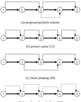
Figure 3.2 shows different jump pointer creation algorithms. A circle represents a dynamic instance of a recurrent load (pointer load). Bold arrows indicate pointer dereferences and all other arrows show prefetches. If it is a dashed line, it means that it doesn’t need a pointer stored in a table and that prefetches can be issued after current instance’s value is loaded. If it is a solid line, it means that it needs a pointer stored in a table and that prefetches can be issued after current instance’s address is available.

1 2 3 4 5

(a) proposed prefetch scheme

1 2 3 4 5

(b) pointer cache [12]

1 2 3 4 5

(c) chain jumping [44]

1 2 3 4 5

A circle represents a dynamic instance of a recurrent load (pointer load). Bold arrows indicate pointer dereferences and all other arrows show prefetches. If it is a dashed line, it means that it doesn’t need a pointer stored in a table and that prefetches can be issued after current instance’s value is loaded. If it is a solid line, it means that it needs a pointer stored in a table and that prefetches can be issued after current instance’s address is available.

Let’s look at the diagram in terms of storage requirement and timeliness of prefetches for prefetching nodes 3, 4, and 5. Assume that nodes 3, 4, and 5 incur cache misses.

Pointer cache [12] requires space for three pointers, and prefetches may not be able to fully eliminate the cache misses if there are not enough independent instructions to hide prefetch latencies. Jump pointer [44] also requires three pointers, but prefetches are issued earlier. When node 1’s address is available, prefetch for node 3 is issued. In this way, two different accesses are overlapped. With the aid of jump pointers, it is more probable that all misses are eliminated. Dependence-based prefetching [43] requires no space for pointers. Even though it requires space for dependence checking and storing, this is generally smaller than the space for jump pointers. Although this prefetcher is the least demanding in terms of space, it has the worst prefetch timing. Since prefetch for node 3 is issued after node 2’s value is available, there is not much chance for the cache miss of node 3 to be completely hidden.

The proposed prefetcher requires space for only two pointers. Nodes 3 and 5 are prefetched in the same way they are prefetched by jump pointers, but node 4 is prefetched differently. Prefetching node 4 doesn’t require a jump pointer; instead it is prefetched by a chain prefetching mechanism. When prefetched data for node 3 comes in, prefetch for node 4 is triggered. The address for node 4 is computed from the prefetched data for node 3.

3.3.3. Filtering mechanism

The filtering mechanism is placed between the processor and the CT in Figure 3.1. In figure 3.3, it is in the correlation identification unit (CIU). A table plays a role of the filtering mechanism, and it is called frequently missed load table (FMLT). Its main job is filtering out infrequently missing loads, so that the rest of the prefetching mechanism can deal with only frequently missing loads. This mechanism uses a simple counter, in which the number of misses of each static load is recorded. When a counter value is bigger than a predefined threshold, it is identified as a frequently missing load (FML) and sent to PPW to find its producer in the list of preceding loads. The filtering mechanism resets the entire table if a predefined number of FMLs have been identified since the last reset. In this way, only the most frequently missing loads can be identified as FMLs, enabling efficient utilization of limited resources placed after FMLT. There are two thresholds in this mechanism: the number of FMLs that triggers FMLT reset, and the number of misses that draws a line between frequently missing loads and infrequently missing loads. Since each application has its own threshold values that work the best for it, dynamically adjusted thresholds may be necessary. This is left for future research.

addresses have not yet been seen.

For dependence-based prefetching scheme, there needs to be a way to combine it with stride prefetching. Since only a load can be a producer, direct-dependence-based prefetching is not able to perform stride prefetching as is. In order to implement the stride filtering mechanism, FMLT has stride field, previous address field, and stride confidence field. Stride field is for storing previous stride and is compared with current stride computed from current address and previous address field. If the current stride is the same as the previous stride, stride confidence is incremented. Otherwise, stride confidence is decremented. If a load is identified as FML and its stride confidence is high enough, instead of being sent to PPW, it is inserted into CT. To indicate such a stride pattern, there is a field for a consumer called ‘stride’. If this is set to one, it means the consumer is for stride prefetching.

3.4. Implementation

In this section, hardware implementation details are presented. The proposed prefetcher is composed of four parts: correlation identification unit (CIU), correlation table (CT), jump pointer creation unit (JPCU), and jump pointer table (JPT). The interactions of these components with themselves, with a processor, and with the memory hierarchy are shown in Figure 3.3.

producer load are dynamically learned by means of incrementing or decrementing counters. When CT is looked up by the processor, these counters are read and an appropriate action is taken. CT is looked up by the processor, whenever a load’s effective address is available. If a stride is detected in a producer’s effective address, a prefetch request is queued in the prefetch request queue (PRQ). If a producer is confirmed as a recurrent load, JPT entries are generated by JPCU and stored in JPT. Every prefetch request is queued in PRQ and sent to L2 cache. When a prefetched block is returned from L2 cache, it is stored in the prefetch buffer. This buffer is accessed by the processor in parallel with L1 cache.

Figure 3.3. Organization of the Proposed Prefetcher

3.4.1. Inserting into CT

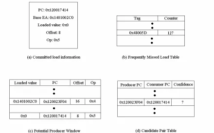
CIU is responsible for generating CT entries and inserting them in CT. The entries to be inserted into CT must have the following two properties. First, the consumers of the entries should miss frequently in the L1 cache, making the processor stall. Second, consumer-producer relations must be strong. CIU is made up of three tables: frequently missed load table (FMLT), potential producer window (PPW), and candidate pair table (CPT).

FMLT is in charge of pinpointing static load instructions that miss in L1 cache frequently. FMLT is updated by committed loads from the processor, and keeps track of the number of misses per static load instruction. If the number of misses reaches a predefined threshold, it resets the counter and sends a signal to PPW. PPW holds a list of recently committed load instructions’ PCs and loaded values in order to facilitate finding producers. The signal from FMLT activates the pairing logic in PPW that tries to find a matching producer for a given effective address from the processor. When the signal is high, both PPW update and pairing are conducted, but when the signal is low, only updating PPW is performed. If a producer-consumer pair is formed, it is then sent to CPT. CPT records the number of times a specific pair has been identified. Only pairs that have strong correlations between their producer and consumer are inserted into CT. FMLT and CPT also reduce the number of CT accesses, reducing conflicts on the write port of CT.

to 7, which is the threshold for inserting into CT, as depicted in Figure 3.4(d). This series of actions describes the mechanism of inserting an entry into CT.

Integrating a plain stride prefetcher into CT can be easily done. Even though the producer is not found for a consumer, an entry is created in CT with its PC as the producer’s PC. The entry is updated by subsequent instances of the consumer; if the consumer has stride pattern in its address stream, it will be learned and prefetches will be issued based on it.

Figure 3.4. Example of Correlation Identification Unit

3.4.2. Updating CT

pattern, either stride or recurrent, is identified for a producer load, this pattern is utilized to make the prefetch engine run ahead of the processor, making it more probable that prefetched data arrive before they are accessed.

If the updating load experienced an L1 cache miss, consumer loads are searched against its PC. Searching all consumer loads may take many cycles, but JPT update occurs infrequently. For pointer-intensive benchmarks such as health and mcf, JPT update occurs once per 22 cycles for mcf, and once per 100 cycles for health.

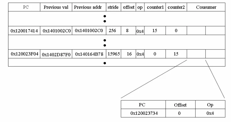
If a match is found and corresponding producer has been identified as a recurrent load, JPT can be updated. CT sends the PC of the corresponding producer to JPCU, and JPCU sends two addresses to JPT. In JPCU, there are 16 FIFO queues, each of which corresponds to a load that has been identified as a recurrent load. These queues are used to record effective addresses and loaded values of up to eight most recently committed instances − in other words, for each recurrent load, up to eight most recently committed instances are stored. For a given PC, JPCU finds the right queue that is assigned to the PC, gets two addresses from the queue, and sends them to JPT. Jump pointer distance is a predefined constant, used for picking up the two addresses. Let’s assume the distance is set to i. The first address is the loaded value of the most recent element of the queue, and the second address is the address of the i-th element from the tail. The first address is to be stored in JPT, and the second address is used to get an index to JPT. Figure 3.5 illustrates this mechanism. The address of the upper entry (0x1401017D8) of the queue is used for indexing into JPT, and the loaded value of the most recent entry, which is the lower entry (0x1402D87F0) of the queue in the figure, is written to JPT.

address can be computed by adding the consumer’s offset to the first address. Therefore, prefetching the address computed from the first address can eliminate the cache miss of the consumer.

Figure 3.5. Example of Jump Pointer Creation Unit and Jump Pointer Table

3.4.3. Looking up CT

CT plays two roles. It detects producers’ patterns, and it works as storage of consumer pairs. One producer can have multiple consumers, which is common in producer-consumer relationships. Figure 3.6 shows two entries of a CT. Counter1 represents the confidence of the stride pattern, and counter2 represents the confidence of the recurrent pattern.

The upper entry in Figure 3.6 has a stable stride pattern, so a prefetch address is computed from the stride and consumer’s offset. The lower entry has a recurrent pattern, so the current effective address will be used to index into JPT. The address returned from JPT is added to a consumer’s offset to form a prefetch address.

Figure 3.6. Example of Correlation Table

3.4.4. An alternate CT structure

The structure of the CT presented earlier is ineffective for storing consumers per producer. From experiments, it is found that only a few producers have more than two consumers, and this finding suggests that allowing a producer to have more than two consumers is wasting precious silicon estate. However, it should be noted that those producers with more than two consumers often contribute to performance improvement and that to harvest the full potential of them, all of their consumers should be stored. Therefore, all consumers should be stored in more effective way.

One such way is to divide the CT into two tables: producer table and consumer table. In this way, searching the consumers for creating jump pointers can make more efficient. In the producer table, each producer has a set of indexes to the consumer table. Each index points to a consumer of the corresponding producer. Since an index is much smaller than a consumer’s information, this approach can reduce space overhead. Each entry in the consumer table also has an index to the producer table. This index points to the corresponding producer. This facilitates jump pointer creation.

When an entry is created in the CT, indexes to the both tables are first determines and the corresponding entries are updated. Indexes to the tables are also stored. When the CT is updated, the producer and the consumer tables are searched in parallel. If a match is found in the producer table, the producer entry is updated. If matches are found in the consumer table, jump pointers are created. When the CT is looked up for generating prefetches, only the producer table is probed. If a match is found, the stored indexes in the producer entry are used to access its consumers.

performance improvements. Because accesses to the tables are serialized, a lookup operation may take more cycles with the new CT structure.

3.5. Evaluation

In this section, we experimentally evaluate the effectiveness of the proposed prefetch mechanism. Section 3.5.1 describes benchmarks used for evaluation and simulator architecture such as processor core configuration, memory hierarchy configuration, and prefetcher configuration. In section 3.5.2, we evaluate several hardware-based jump pointer creation mechanisms by comparing them with naïve implementation. Section 3.5.3 contains experimental results for varying jump pointer distance. In section 3.5.7, we analyze our proposed scheme in terms of IPC, and breakdown of memory operation handling.

3.5.1. Experimental setup

Our experiments were performed using the SPEC2K integer benchmark suite, the Olden benchmark suite, and the deltablue pointer-intensive benchmark. From the SPEC2K integer benchmark suite, bzip2, gap, mcf, parser, and twolf were used. From the Olden benchmark suite, bisort, health, mst, treeadd, and tsp were used. All other benchmarks not used in this experiment don’t show noticeable improvement, so the results for them are not presented. Olden and deltablue benchmarks were simulated to completion. For SPEC2K benchmarks, a representative 100 million instructions were simulated, which were identified by SimPoint [48]. SPEC2K benchmarks use reference inputs.

al. [46]. Simulated processor configuration is summarized in Table 3.1.

Table 3.1. Simulation parameters

Processor core configuration 5 stage pipeline; 4 way superscalar; 128 entry Reorder buffer; 32 entry

load-store queue, hybrid (bimodal + 2 level) branch predictor; 4 integer

units, 2 multiplication units, 1 division unit;

Memory hierarchy configuration 64K, 2way, 32B, 16 MSHR, 2 cycle L1 data cache; 64K, 2way, 32B, 16

MSHR, 1 cycle L1 instruction cache; 1M, 8way, 64B, 16 MSHR,15

cycle L2 cache; 100 cycle memory latency; 2:1 frequency ratio, 32B

bandwidth L1-L2 bus; 4:1 frequency ratio, 16B bandwidth L2-mem bus;

Prefetcher Configuration Direct-mapped, 128 entry FMLT; Direct-mapped, 64 entry CPT;

Fully-associative 128 entry PPW; Fully Fully-associative 64 entry CT; 32 entry

PRQ; 128 entry(4KB), 32B Prefetch buffer;

3.5.2. Effectiveness of hardware-based JPT creation mechanism

In a pure hardware implementation of JPT, the space requirement is the most critical factor. In this section, several mechanisms designed to reduce the space requirement are evaluated.

The first mechanism is to create a jump pointer only for a missed dynamic instance. Since not all instances incur cache misses, it can save some space by not creating unnecessary jump pointers for instances that hit in L1 cache.

jump pointer of distance n is created, and the subsequent n-1 instances are prefetched via chain prefetching. Since the following n-1 instances are already covered, new jump pointers for them shouldn’t be created. Therefore, there should be a mechanism that distinguishes covered instances from non-covered instances. This can be achieved by recording the chain length of each pointer in the JPT, and using that information when the same jump pointer is encountered again. If a jump pointer is about to be created for an instance whose position is less than the stored chain length from the jump pointer that has already been learned and was encountered again, jump pointer creation is canceled.

The third mechanism is a jump pointer blocking mechanism. There are some static loads whose effective addresses don’t repeat. Since the jump pointer approach relies on repeated patterns of address streams, it is not able to obtain any benefit from this kind of load. In addition, these loads waste space, preventing useful jump pointers from being inserted into JPT. This mechanism effectively blocks creation of jump pointers for non-repeating loads by keeping track of the number of jump pointers created and the number of times prefetch requests are made for each CT entry. If the number of created jump pointers is large and the number of prefetch requests made for the pointers is small, the corresponding CT entry is blocked from generating jump pointers. As a side effect, this may end up blocking creation of useful jump pointers. This happens for loads that have a large number of elements in their repeating sequences. To prevent this, the block is removed when the number of prefetch requests exceeds a certain threshold. This way, loads that don’t contribute to prefetch are blocked, and loads that have potential for performance improvement are allowed to create jump pointers.

Table 3.2. The number of jump pointers created for mcf and health

JP created for cache

miss

JP created with chain

mechanism

Unconstrained JP

creation

mcf

69,257 66,917 82,735

health

92,569 72,490 131,001

For mcf, the first and the second mechanisms create 16% and 19% fewer jump pointers, respectively, than the case where jump pointers are naively created for all dynamic instances. For health, the two mechanisms achieve 30% and 45% space savings, respectively. The difference between the cache miss and chaining mechanisms grows if there are many consecutive misses, allowing chain mechanism to take advantage of them. Sometimes prefetch chains are broken for two reasons. First, recurrent loads often load zeros, which happens when the control flow changes. Second, another instruction in a seldom-used different control path produces an effective address that interrupts the stable pointer chasing pattern. If a prefetch chain is broken, the chain ends there and a new jump pointer is created. Since health has longer and fewer prefetch chains than mcf, space saving is greater than that of mcf.

Figure 3.7 shows IPCs of different mechanisms, normalized to the IPC of the no-prefetch case. For unlimited JPT, naïve creation is the best, followed by missed-instance-only creation and chain-prefetch-aware creation. Naïve creation beats the other two simply because it has more jump pointers. For 32k JPT, chain-prefetch-aware creation performs the best. Even though the number of jump pointers created for missed-instance-only creation and chain-prefetch-aware creation are similar (mcf), chain-prefetch-aware creation actually prefetches more because of chain prefetching.

repeat. For parser, mst, tsp, the blocking mechanism reduces space requirements dramatically with little performance degradation, but they don’t benefit much from jump pointers.

0.5 0.6 0.7 0.8 0.9 1 1.1 1.2 1.3 1.4 1.5 1.6 1.7 1.8 1.9 2 2.1 mcf health re la tiv e I PC no-prefetch unlimited JPT (naïve) unlimited JPT(miss_only) unlimited JPT(chain) 32K JPT (naïve) 32k JPT (miss_only) 32k JPT (chain) 32k JPT (chain+blocking)

Figure 3.7. The effectiveness of JP creation mechanisms in terms of IPC

3.5.3. Jump pointer distance

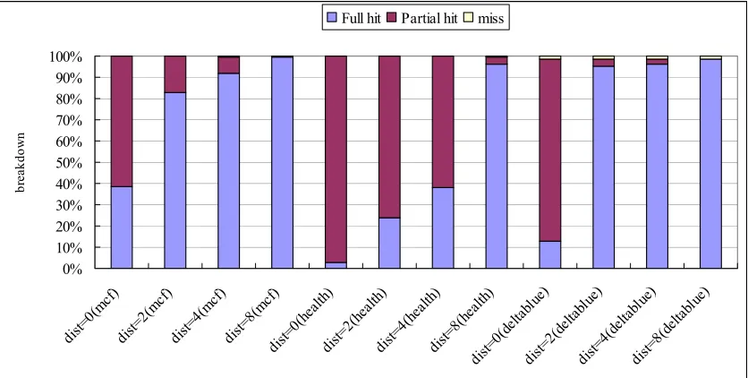
0% 10% 20% 30% 40% 50% 60% 70% 80% 90% 100% dist=0 (mcf ) dist= 2(mc f) dist= 4(mc f) dist= 8(mcf ) dist= 0(he alth) dist= 2(he alth) dist= 4(hea lth) dist= 8(he alth) dist= 0(de ltablu e) dist= 2(de ltabl ue) dist= 4(de ltabl ue) dist=8 (delt ablue ) br ea kd ow n

Full hit Partial hit miss

Figure 3.8. Prefetch reference breakdown with varying jump pointer distance

As jump pointer distance increases, the number of full hits also increases and the number of partial hits decreases. This is because prefetches can be issued much earlier, making the prefetches arrive at the prefetch buffer before they are used. Note that the rate at which the number of full hits grows is different for each benchmark. For mcf and deltablue, the number of full hits grows fast but for health, it grows slowly.

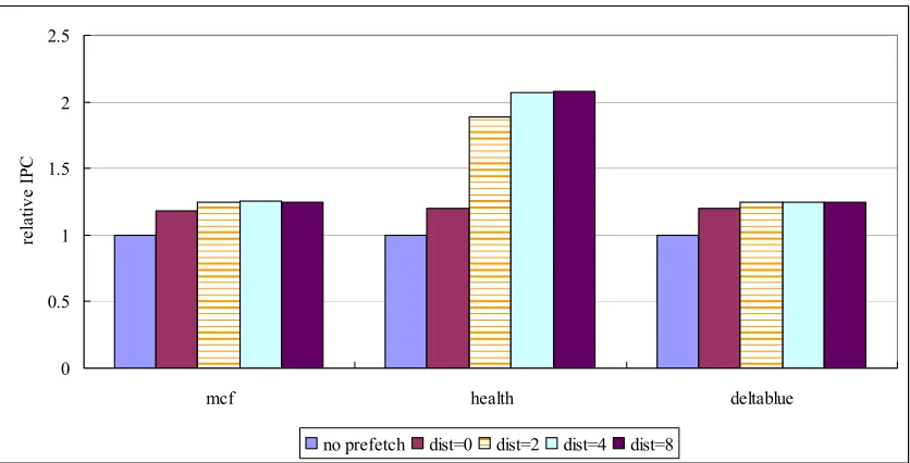
Figure 3.9 shows the IPC. At jump pointer distance two, IPCs of mcf and deltablue already saturate, whereas IPC of health saturates at distance four. This is in accordance with what we found in figure 3.8.

0 0.5 1 1.5 2 2.5

mcf health deltablue

re

la

tiv

e IP

C

no prefetch dist=0 dist=2 dist=4 dist=8

Figure 3.9. Influence of jump pointer distance on IPC

3.5.4. Jump pointer accuracy

Jump pointers are used to predict future addresses that a processor is likely to access. Therefore, accuracy of jump pointers is an important factor that determines prefetcher efficiency. If the accuracy is low, the cache could be polluted with useless data, and demand fetches may be delayed due to resource contention with useless prefetches.

Figure 3.10 shows the accuracy of jump pointers with varying jump distance. A jump pointer is a pointer that points to the address of a future dynamic instance, and it is associated with the address of the current dynamic instance. Jump distance is the number of dynamic instances between the instance that the pointer is associated with and the instance the pointer points to. The x-axis represents jump distance and the y-axis shows jump pointer accuracy. Each line indicates a load that jump pointers are created from. The numbers of the lines are the last four decimal digits of the loads.

and their accuracies are measured.

To measure the accuracy, the stream of effective addresses and loaded values for each load instruction is generated and analyzed. Jump pointers for a given distance are created and stored in a table. For each jump pointer, two addresses are stored: the address the pointer is created from, and the address that the pointer references. When the address the pointer references is seen again, the stream of address/value pair is checked with the given jump distance. If the same addresses are paired again, the hit counter is incremented. Each effective address and loaded value pair updates the jump pointer table to learn changes in the LDS.

The graph shows that accuracy drops linearly as jump distance increases. On average, 86% - 87% accuracy is achieved with distance 8, but for some static load instructions, accuracy drops below 75% with distance 8. This leads us to conclude that jump distance needs to be as small as possible, as long as it is still large enough to hide cache misses.

0 20 40 60 80 100

dist 0 dist 2 dist 4 dist 6 dist 8

A cc ur acy ( % )

Load 1 Load 2 Load 3 Load 4 Load 5 Load 6 Load 7 Average (a) Mcf

0 20 40 60 80 100

dist 0 dist 2 dist 4 dist 6 dist 8

A ccu ra cy ( % )

Load 1 Load 2 Load 3 Average

(b) Health

Figure 3.10. Accuracy with varying jump distance

3.5.5. Sensitivity of the correlation table to ports and access latency

requests, a read operation is performed. Since the CT is accessed quite a lot due to these updates and lookups, the impact of the number of ports on the CT and access latency of the CT need to be studied.

Figure 3.11 shows the impact of the number of ports on the CT to overall IPC. The number of ports is varied from one read and one write port up to eight read and eight write ports. To measure the influence of modeling the ports, a result without modeling the ports is included. Also, a case with a set of small buffers, which temporarily stores accesses to the CT, is presented. The y-axis represents relative IPCs normalized to the IPC of the case without modeling the ports.

For twolf, the number of ports doesn’t matter at all. But for mcf and health, when only one read and write port are available, significant IPC decrease is observed. This is because some of the crucial producers are not identified due to contention on the ports. If a set of small buffers are placed to temporarily store read and write operations respectively, one read port and one write port are turned out to be sufficient.

0 0.2 0.4 0.6 0.8 1 1.2

gap mcf parser twolf health mst treeadd deltablue

re

lative IP

C

1r, 1w 2r, 2w 4r, 4w 8r, 8w 1r, 1w with buffer not modeled

0.8 0.85 0.9 0.95 1 1.05

gap mcf parser health mst treeadd deltablue

re

la

tiv

e IP

C 2

4 6 8

Figure 3.12. Sensitiveness of the CT to its access latency

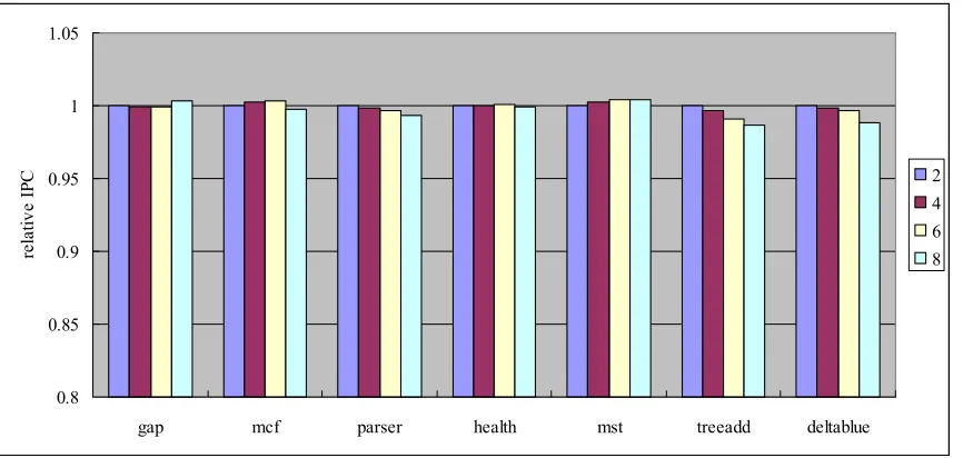
3.5.6. Sensitivity of the potential producer window to ports and access latency

The potential producer window (PPW) is a FIFO queue, in which committed loads’ information is stored. consumer to producer matching is performed in the PPW, and this action requires traversing the queue until a corresponding producer is found. To accurately implement the PPW, ports and access latency of the PPW are modeled. For example, if the length of a traversal is three PPW entries and access latency is two cycles, the corresponding port will not be ready in six cycles. If there is no available port, the corresponding request is simply discarded. For this experiment, write port is assumed to be sufficient. This is because writing multiple entries per a cycle can be implemented relatively inexpensively. Therefore, only the read ports are considered.

producer matching doesn’t occur frequently due to the filtering mechanism and updating the CT is not in a critical path.

Figure 3.14 presents the sensitiveness of the PPW to its access latency. Y axis represents relative IPCs normalized to the IPC of the case where the access latency is set to one. X axis represents the access latency of the PPW, and the latency varies from one cycle to four cycles. All benchmarks are not sensitive to the access latency of the PPW. The same reasons as the number of port experiment apply. Comsumer to producer matching doesn’t occur frequently enough to have the access latency influence overall IPC, and updating CT is not in a critical path.

0.8 0.85 0.9 0.95 1 1.05

gap mcf parser health mst treeadd deltablue

re

la

tiv

e IP

C 1

2 3 4

0.8 0.85 0.9 0.95 1 1.05

gap mcf parser health mst treeadd deltablue

re

la

tiv

e IP

C 1

2 3 4

Figure 3.14. Sensitiveness of the PPW to its access latency

3.5.7. Effectiveness of the proposed prefetcher

To evaluate the effectiveness of the proposed prefetcher, systems with 1M L2 cache and 2M L2 cache are compared with the system with 1M cache and the prefetcher. Two versions of the prefetcher are presented: one with 32K JPT, the other with 64K JPT. The prefetcher with 32K JPT takes about 512KB, and the one with 64K JPT consumes about 1MB. The prefetcher has chain mechanism described in section 3.3.2, jump pointer distance is set to four, and JPT access time is set to 18 cycles for both sizes.

Figure 3.15 presents breakdown of prefetch hits: stride-based prefetch, jump pointer-based prefetch, and chain-prefetch. Each bar has three regions, each of which indicates a mechanism that contributes to prefetch hits. Note that each benchmark has a different number of prefetch hits.

0% 20% 40% 60% 80% 100%

gap mcf parser twolf bisort health mst treeadd tsp deltablue

br

ea

kdow

n

normal stride normal jp chain

Figure 3.15. Breakdown of prefetch hits: stride-based prefetch, jump pointer-based prefetch, and chain-prefetch

Figure 3.16 shows the IPCs of seven different configurations. The first two bars represent the IPCs of two different L2 cache sizes: 1MB and 2MB without prefetching. The next three bars are IPCs of three prefetching schemes: he proposed prefetching with 64K-entry JPT, original dependence-based prefetching (DBP) [43], and jump-pointer prefetching (JPP) with 64K-entry JPT [44]. The last two bars show IPCs of perfect L2 Cache and perfect L1 Cache, respectively. In this section, all prefetching mechanisms are evaluated with dedicated prefetch tables and 1MB L2 cache. (Storing the prefetch table in L2 is evaluated in the next section.) The IPCs are normalized to that of 1MB L2 cache without prefetching.

For some benchmarks such as gap, treeadd, and equake, going from 1M L2 cache to 2M L2 cache doesn’t improve performance more than 2%. This means that the advantage of the bigger L2 cache size is not effectively utilized to improve performance.