Environmental Analysis of Swine Waste Management Technologies Using the Life-Cycle Method

ENVIRONMENTAL ANALYSIS OF SWINE WASTE MANAGEMENT TECHNOLOGIES USING THE LIFE-CYCLE METHOD

Evan M. Griffing, Michael R. Overcash, and Seungdo Kim

Department of Chemical Engineering College of Engineering

North Carolina State University Raleigh, NC 27695

The research on which this report is based was financed in part by the United States Department of the Interior, Geological Survey, through the North Carolina Water Resources Research Institute.

Contents of the publication do not necessarily reflect the views and policies of the United States Department of the Interior, nor does mention of trade names or commercial products constitute their endorsement by the United States Government.

WRRI Project No. 701 82 and 70193 USGS Project No. 1434-HQ-96-GR-02689

ABSTKACT

An important broader environmental profile of swine waste management options is created using life-cycle techniques when compared to the focused criterion of ammonia emissions. In order to utilize the life-cycle approach, mass and energy balances were created for each of four swine waste management technologies. Also, these mass and energy balances were extended to include the entire supply chain of any electricity o r chemicals used or generated when managing swine waste. This database enables decision makers to examine hidden benefits or impacts of new technologies for swine waste management.

The basis for comparing new technologies is in relation to the existing barn, lagoon, and land application (effluent and sludge) system. These systems were each analyzed b y mass and energy balances as well as by extensive literature compilations. Overall, a mass balance approach (when essential variables are measured) was accurate and considerably less expensive as a means to estimate ammonia volatilization.

TABLE OF CONTENTS

ACKNOWLEDGEMENTS ABSTRACT

TABLE OF CONTENTS LIST OF FIGURES LIST OF TABLES

SUMMARY AND CONCLUSIONS RECOMMENDATIONS

INTRODUCTION

EMISSION SAVINGS FROM UTILIZING SWINE WASTE TO REPLACE COMMERCIAL FERTILIZERS

Fertilizer sources: national average Emission allocation

Natural resource consumption

AMMONIA AIR EMISSION FROM THE BARN NITROGEN LOSSES IN LAND APPLICATION Nitrogen losses fiom lagoon effluent application Nitrogen losses fiom surface application

Nitrous oxide emissions during land application

Land application emissions used in the life-cycle calculations ANAEROBIC LAGOON

Average swine waste data

Calculation of the settling coefficient Seepage rates from the lagoon

Nitrogen loss in the lagoon

Estimates of nitrogen loss based on a mass balance Direct measurement of ammonia flux

Measurements by Aneja et al. (2000, 2001) Measurements by Todd et al. (2001)

Measurements by Harper et al. (2000,2004) Measurements by Lim et al. (2003)

Comparison of direct measurement techniques to the mass balance model Methane and carbon dioxide emissions

Inventory data for the traditional anaerobic (ana) lagoon BIOLOGICAL AERATED FILTER PROCESS (BAF)

Model

Energy requirements for aeration Inventory data for baf process

COVERED ANAEROBIC LAGOON (CAL) Data from cheng et al. (2000)

Energy generated from captured methane Inventory data for the covered lagoon

DIRECT APPLICATION OF RAW SWINE WASTE COMPARISON OF WASTE TECHNOLOGIES

. . .

111 v vii ix xi

_...

X l l l xvii 1

LIST OF FIGURES

Figure 41. Ammonia emissions fiom life-cycle evaluation of swine waste management

Technologies v

Figure A 2 Global warming emissions (COz equivalents) from life-cycle evaluation of Figure 1. Figure 2. Figure 3. Figure 4. Figure 5. Figure 6. Figure 7. Figure 8. Figu-2 9. Figure 10. Figure 1 1 . Figure 12. Figure 13. Figure 14. Figure 15. Figure 1 6 . Figure 1 7. Figure 1 8. Figure 19. Figure 20. Figure 2 1. Figure 22. Figure 23. Figure 24. Figure 25. Figure 26. Figure 27. Figure 28. Figure 29. Figure 30. Figure 3 1.

Figure 32. Figure 3 3.

Figure 34. Figure 35. Figure 36. Figure 37. Figure 3 8. Figure 39. Figure 40. Figure 4 1.

swine waste management technologies v

Life-cycle boundary, chemical emissions, and energy use/generation 2

The inputs required to produce N- fertilizer 7

Allocation of the manufacture of 1000 kglhr of DAP 8

Supply chain of commercial fertilizer 10

The raw material source tree for nitrogen 11

Nitrogen loss versus

f

(TAN:TKN ratio) during irrigation 19 Ammonia emissions for surface application methods versus applied TAN 22

Ammonia emissions for injection methods versus applied TAN 23

Ammonia emission versus applied TKN for surface spread waste 23

Ammonia emission versus applied TKN for injected waste 24

Ammonia emissions versus f (TAN:TKN ratio) from surface spreading 25

Ammonia emissions versus f (TAN:TKN ratio) from injection 26

Mass transfer model of anaerobic lagoon 3 1

Nitrogen accumulation per unit live weight in anaerobic lagoon sludge 34

The settling coefficient for nitrogen (percent into sludge) 35

Model for single-stage recycle lagoon 36

Comparison of mass transfer coefficient over all lagoons with full year data 49 Comparison of percent loss of TKN over all lagoons with full year data 50 Schematic of the Ekokan aerated biofilter used by Westerman et al. (2000) 60 COD removal in a generic aerated biofilter process 62

Fate of nitrogen in an aerated biofilter 63

Model for phosphorus and potassium in the biofilter 65

Model for CAL 71

The covered lagoon system studied by Cheng et al. (2000) 72

Nitrogen content that is conserved and utilized by plants 83

Total energy use 85

Coal use 86

Crude oil use 87

Natural gas use 87

CH4 emission 89

CH4 emission by life-cycle phase ₈₉

C02 emission (prior to C02 loss from terrestrial system) ₉₀

COz emission by life-cycle stage (prior to CO2 loss fiom terrestrial system) 90

CO emission 91

N 2 0 emission 92

N 2 0 emission by life-cycle stage ₉₂

NH3 emission 94

Ammonia emission by process step ₉₄

NOx emission 95

SO, emission 96

Figure 42. NO3- emission fiom energy consumption and generation Figure 43. BOD emission

LIST OF TABLES

Table 1.

Table 2. Table 3. Table 4. Table 5. Table 6.

Table 7. Table 8. Table 9.

Composition of commercial fertilizer The composition of NPK

Chemical make up of fertilizer by primary nutrient content Natural resources used to create 1000 kg of N in fertilizer

Emission factors for nitrogen loss in the barn and storage facility Nitrogen loss during irrigation of lagoon effluent

Ammonia and NzO losses from surface spreading techniques Ammonia and N 2 0 losses from injection methods

TAN:TKN ratio fiom raw waste and surface spreading studies

Table 10. The f value for lagoon sludge 27

Table 1 1. Summary of ammonia volatilization losses during land application 28

Table 12. Summary of N 2 0 emissions during land application 29

Table 13. Land application losses used in the life-cycle inventory 29 Table 14. Summary of data on swine waste nitrogen content from Barker (2002) 33 Table 15. Reported or estimated lagoon parameters used in mass balance 39 Table 16. Results from mass balance model for single-stage lagoon 39 Table 17. Estimate of standard deviation of each parameter in mass balance 40 Table 18. Contribution of each term in the calculation of the mass transfer coefficient 41

Table 19. Average ambient and lagoon temperatures 43

Table 20. Conversion of ammonia flux to a percent loss of TKN 44

Table 2 1. Ammonia emission data from Aneja et al. (200 1) 44

Table 22. Integration of emissions based on fitting equation fiom Aneja et al. (2001) 45 Table 23. Calculation of ammonia emissions from Todd et al. (2001) 46

Table 24. Calculations of N2 flux based on Harper et al. (2000) 47

Table 25. Calculation of yearly average emissions for Harper et al. (2004) 48

Table 26. Summary of Lim et al. measurements on lagoon emissions 49

Table 27. Average percent Nitrogen loss and mass transfer coefficient for each

measurement method 50

Table 28. Conversion and yield of carbon content into methane and carbon dioxide 52 Table 29. Biogas formation data from covered and traditional anaerobic lagoons 54

Table 30. Biogas formation data fi-om digesters 54

Table 3 1. Scenarios for the anaerobic lagoon 57

Table 32. LC1 summary for anaerobic lagoon scenarios 57

Table 33. Data on solid/liquid separations of swine waste 61

Table 34. Fate of carbon in BAF 62

Table 35. Summary of nitrogen factors 63

Table 36. Phosphorus and potassium factors in the biofilter 65

Table 37. Nutrient content in municipal waste sludge compared to data from biofilter

treatment of swine waste 66

Table 3 8. Energy requirements for aeration of waste 68

Table 39. BAF cases used in life-cycle analysis 69

Table 40. Summary of nutrient emissions and energy use for each BAF case 69

Table 41. Electricity and heat generation from biogas 74

Table 42. Scenarios for emission calculations of CAL 75

Table 44. Scenarios for direct application (DA) of swine waste Table 45. Emission summary for each direct application scenario Table 46. Anaerobic lagoon scenarios for life-cycle inventory Table 47. Scenarios for aerated treatment

Table 48. Scenarios for the covered anaerobic lagoon Table 49. Scenarios for direct application of swine waste

Table 50. Comparison of emissions and resource use for each technology Table 5 1. Energy consumption associated with fertilizer production Table 52. Global warming potential

SUMMARY AND CONCLUSIONS

The comparison of swine waste management technologies can be done in a number of ways (e.g., economics, emissions of a single chemical such as ammonia, in terms of total environmental impact, etc.). The latter is referred to as the net environmental benefit or life-cycle approach. Use of a life-cycle concept attempts to understand the transfer or shifts in pollution that often occur in complex systems such as the swine production industry.

The Water Resources Research Institute of the University of North Carolina has funded a parallel study to the large Attorney GeneralBmithfield Agreement research effort. The goal of the WRRI project is to determine for a small number of swine waste management alternatives, what life-cycle results would occur, and compare that to the results from decision making for ammonia emissions. Four swine waste management technologies were investigated:

1. conventional lagoon and spray irrigation (with lagoon solids removal and land application when full),

2. covered lagoon with spray imgation, utilization of methane production for electricity, and lagoon solids removal and land application when full,

3. biological aerated filter process with land application of effluents and solids, and 4. Harvestore collection and land application of raw waste.

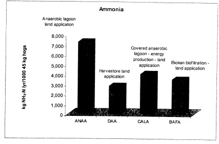
An engineering and science approach was used to assess the energy (usually electricity) and emissions from each of these technologies. Because a life-cycle approach was used, all related supply chain emissions and energy requirements were also added. Thus, when electricity is used, the emissions from electrical power generation are included. When swine waste NPK are land applied, emissions and energy requirements from industrial plants for NPK are correspondingly reduced, creating an environmental benefit. Analysis of these technology comparisons was done for a number of environmental parameters, but in this summary, two are highlighted. The first is the ammonia emissions to the air, and the second is the impact on global climate change potential (a combined effect of C02, methane, and nitrous oxides, using scientific rules for combining these emissions and expressing the effect as equivalent COz. These results are provided in Figures 1 and 2.

...

Figure A 1 : Ammonia emissions fi-om life-cycle evaluation of swine waste management technologies

Anaerobic lagoon land application

Ammonia

Covered anaerobic lagoon - energy production - land

application Bokan biof iltration land application Harvestore land

application

ANAA DA A BA FA

Figure A2: Global warming emissions (C02 equivalents) from life-cycle evaluation o f swine waste management technologies

Anaerobic lagoon land application

GWP

b k a n biof iltration - land application

Covered anaerobi

Harvestore land production - land

ANAA DAA CALA BA FA

The life-cycle approach shows that changing swine waste management technologies results in two clear geographic transfers of pollution. First, using ammonia emissions as the criterion for technology choice (Figure 1 ), the Ekokan biofiltration is slightly better than the covered lagoon and significantly better than the current lagoon-land application system. However, when one looks at global warming emissions, the Ekokan system has a substantially higher impact than the new technologies of the covered lagoon or the direct land application. Thus, there is a geographic shift from ammonia emissions at the swine site, to larger emissions at the power generation facilities.

The second shift is from one form of emissions to another. In this case, the shift is fi-om ammonia in air to the constituents comprising global warming potential. This is referred to as chemical or pollution shift. In the report, other environmental shifts are documented for these four swine waste management alternatives.

Conclusions

1. A life-cycle approach to swine waste management technologies selection provides the most comprehensive assessment of environmental impact.

2. Mass balance approaches provide more independent measures and lowest cost technique for determining ammonia emissions from most swine waste

management technologies.

RECOMMENDATIONS

1. A mass-balance approach should be used to verify environmental measurements of swine waste management technology. This can identify measured data by comparison to conservative chemicals (such as chloride) and thus increase the public and scientific acceptance of such technology evaluation.

2. Comparisons of swine waste management technologies should look at all significant environmental impacts to assure the solution for one chemical parameter (such as ammonia) does not shift emissions to other media, geographic locations, or chemical impacts.

INTRODUCTION

Swine waste is generally thought of as a waste material. It is an unwanted byproduct of growing swine, and it is expensive to dispose. A current standard method of disposal (the anaerobic lagoon) consists of a holding pond where swine waste is periodically

discharged. The waste separates into a liquid component and a solids component, which settles as sludge in the bottom of the lagoon. The liquid (more frequently) and the solids (infrequently) are periodically removed and distributed to the land as fertilizer. Farmers favor the anaerobic lagoon partly because it effectively removes unwanted nitrogen. Lower nitrogen content means that disposal is cheaper, because shorter transport

distances are required to apply the waste in agronomic levels. However, direct nitrogen emissions from the lagoon in the form of ammonia and/or nitrate are environmental costs. Several other waste management technologies, such as a covered anaerobic lagoon and an aerobic lagoon, exist as alternatives to current procedures. In order to evaluate the e n v i r o c ~ ; : ' ~ ) ' ::-:Y. : it' .':r:c txhnologies, comprehensive calculations of the chemical ernisqir- ?nd enerev reouiremwts to run the lagoon and land distribution processes are Vher. c p : ~ ~ ? r - +-d. rv.;*-c waste is an effective fertilizer and can be used in place of

commercial iertilizers. Therefore, it provides an emission savings related to the amount of fertilizer that would otherwise be required. Common chemically manufactured fertilizers are diammonium phosphate (DAP), ammonia, urea, and potassium chloride. The energy and emissions associated with the production of 1000 kg of each of these chemicals have been calculated. The calculations are performed on each input chemical to each process until the raw materials from the ground have been reached. These calculations are based on process designs and thermodynamic principles as described by Jimenez-Gonzalez et al. (2000). Each of the chemicals noted above is sold and applied as fertilizer. A commonly used mix of commercial fertilizer (NPK) is subdivided and

treated as the basic fertilizer constituents of this mix.

Most processing systems can be broken into housing (barn), treatment (lagoon), and land application steps. It is possible that the methods used in one step may change the

performance of another step. For instance, barn flushing utilizes the effluent from the processing stage. A nitrogen conserving technology may lead to higher ammonia emissions in the barn due to the use of a more nitrogen rich effluent. However, the

literature data is not sophisticated enough to quantify or even predict all of these effects. _. Therefore, we consider each step independently.

We assume that a known amount of waste with a given composition is produced per mass of live animal weight (LAW). At each step, we assume allocation fractions determine what percentage of the input to that step is assigned to a specific fate. For instance, in the lagoon, we assume from literature data that a certain percentage of the input nitrogen is volatilized as ammonia. This is different from assuming that a certain mass of ammonia is volatilized per unit live weight or per unit area in the lagoons. These other bases for quantifying the fate of waste constituents can be related to the percent base only for specific cases.

the literature. Ammonia volatilization from the barn, which is also determined from the literature, is used to calculate the excreted quantity of total Kjeldahl nitrogen (TKN). Energy consumption and generation in the treatment stage and chemical emissions are determined for the anaerobic lagoon and for each alternative treatment technology. The emissions from the treatment step are NH3, N2, N20, C 0 2 , and CH4 in the gas phase, and NH3, P, and K in the liquid phase. Energy is generated in the covered anaerobic lagoon (CAL) or ambient temperature digester, and energy is consumed in the biological aerated filter (BAF). Chemical emissions and raw material associated with energy use are included in the life-cycle inventory. Separate emission factors are calculated for three different land application methods. The liquids are applied by irrigation, and the solids are either applied to the surface, or injected below the surface.

Figurel. Life-cycle boundary, chemical emissions, and energy use/generation

NH,-N bolatilization

Chemical emissions

Chemical emissions

Energy saved (CAL) NH;, N,O

avoided off-site emissions

fuel use and emissions not included

f Seepage loss o f N,P,K Energy used (BAF)' (AN A, CAL) off-site emissions

Chemical emissions

Energy

and off-site emissions Raw materials

b

Carbon losses from the barn and land application (methane and carbon monoxide) are excluded. The losses from the barn are the same for each processing technology;

fertilizer (N,P,K) Fertilizer

manufacture

therefore, there is no effect on the comparison of treatment technologies. Volatile solids destruction does vary considerably between the treatment technologies. This is expected to have an impact on both odors and carbon emissions during land application. Although the effect was not quantified, it should be considered when comparing the life-cycle emissions from the direct application to those of other technologies. Seepage losses in the treatment step are used to determine nutrient conservation. There is some concern about nitrate leaching into the groundwater, and about nutrient transport into the

ecosystem due to seepage. However, it is clear from soil studies that much of the seeped material is filtered by the soil immediately beneath the lagoons. Therefore, the seepage losses are not treated as environmental emissions in the impact assessment. The

transportation from the processing stage to the land application site has a significant economic impact, the environmental impact is small, and these emissions were not included.

The following section explains how the emission credits for chemical fertilizer

replacement are determined. Each of the storage/processing systems considered in this study are used in conjunction with housing and land application steps. Therefore, these steps are considered in the next two sections. The models for each of the

EMISSIONS SAVINGS FROM UTILIZING SWINE WASTE TO REPLACE COMMERCIAL FERTILIZERS

The full benefit from agronomic use of swine waste must include the resource, energy, and emission credits from not manufacturing conventional fertilizers such as

diammonium phosphate (DAP), ammonia, urea, and potassium chloride. The current volume of fertilizer production that is avoided due to application of swine waste is

unknown. Each fann utilizes or disposes of the waste in a different manner. Some farms grow hay on an otherwise unused field, and some plans exist for filling in lagoons and growing trees to remove the accumulated nutrients from sludge in decommissioned lagoons. However, in a 'beneficial reuse' scenario, the waste is applied to land where fertilizer is otherwise needed to maintain crop growth. In this report, we consider the beneficial reuse scenario, and equate swine waste to fertilizer through efficacy of crop growth.

Fertilizer specification and performance are directly related to the amount of primary nutrients (nitrogen, phosphorous, and potassium) that are available to plants. Plant availability, nutrient ratios, and other factors contribute to the capacity to improve crop growth. Most plants utilize nitrogen and phosphorus in a ratio of 8: 1 (N:P) (Adeli et al. 2002). Swine waste effluent typically has less nitrogen than 8: 1. Because it is applied in agronomic quantities of the limiting nutrient, N, phosphorus is applied in excess and accumulates in the soil (Worley and Das 2000; Adeli et al. 2002). Nitrogen in manure is also typically less available to plants than chemical fertilizers (Sharpley et al. 1994; Adeli and Varco 2001). However, in lagoons, a high percentage of organic N is broken down into ammonia, which is readily available (Evans et al. 1977). Swine waste processing technologies further complicate the issue by changing the nutrient ratio and chemical form. For instance, a covered lagoon can maintain the raw waste N:P ratio, and a direct application technology can limit the amount of N that is immediately available to crops. Swine lagoon effluent is often thought of as a waste rather than a resource. As such, it has been applied to land as a disposal method in conjunction to the application of commercial fertilizer. Gangbazo et al. (1995) showed that this practice, which was common in Canada, is environmentally unsound due to the resulting high loading rates. In order to call swine waste a replacement for fertilizer, it is necessary to have empirical comparisons of biological waste (municipal and animal) to chemically produced

fertilizer. Many studies have shown that organic waste performs as well as or better than commercial fertilizer on an applied primary nutrient basis (Chang et al. 1982; Hemphill et al. 1982; Day et al. 1983; Kiemnec et al. 1990; Reed et al. 1991 ; Eghball and Power 1999; Adeli and Varco 200 1 ; Adeli et al. 2002; Al-Kaisi and Waskom 2002). These studies typically compare biological waste to commercial fertilizer based on the agronomic rates of the limiting nutrient (N). Therefore, one could argue that as a replacement for commercial fertilizer, swine waste should only be credited for the

fertilizer value of the limiting nutrient. From a beneficial reuse perspective, the goal is to derive the maximum benefit from recyclable nutrients. In that scenario, swine waste would be supplemented with commercial fertilizer. For instance, lagoon effluent that is low in N could be mixed with ammonia to produce a balanced fertilizer product.

chemical fertilizer and swine waste are typically not being applied in optimal ratios of N, P, and K at all times; therefore, getting the optimal ratio of N:P in reused waste is not necessary for this replacement model to be a fair assessment.

FERTILIZER SOURCES: NATIONAL AVERAGE

The emission savings per unit of primary nutrients must be calculated based on the

national average use of e a ~ h of the fertilizer chemicals as a way to reflect broad (average) agricultural practices. Commercial fertilizer is classified into three types: N fertilizer (nitrogen), P fertilizer (phosphorous), and

K

fertilizer (potassium). Each of these fertilizer types represents the composite of 'source' chemicals, which produce these primary nutrients. These 'source' chemicals are the result of the U.S. agricultural chemicals sector and thus represent an average fertilizer profile. The amount of each chemical used per kilogram of a fertilizer type is based on this national average and is given in Table 1. The chemical fertilizer NPK is shown in the table, because NPK usage is often given in the literature. NPK is really just a composite of ammonia, DAP, and potassium chloride.

Table 1. Composition of commercial fertilizer

r

Fert i 1 izer Type Source Chemical Chemical purity

% of total farm usage of primary nutrient from each source

N (% in each source)

PzOS (% in each source)

I P

(% in each source)

J K ~ O (% in each source) IK (% in each source)

N fertilizer Ammonia Urea

99.7

K fertilizer

-

5

1

- -

For example, 53% of N in fertilization comes from ammonia. The percentage of primary nutrient is calculated based on the product purities listed in the table. For example, 82.3% of pure ammonia is nitrogen, but since the purity is only 99%, the resulting ammonia N percent is 81.5%.

a U.S. production statistics in F A 0 data: N/P20s/K20 basis (Nielsson 1987).

b(Nielsson 1987).

5% impurities (The calculated total mass value is 62.9)

According to the EEC Guidelines (Nielsson 1987), NPK fertilizers must contain at least

3% N plus 5% PzOs plus 5% K 2 0 and at least 20% total nutrients (Ullmann 1985- 1996). For Nutrient ratio 1 : 1 : 1

Typical examples are 15-15-15, 16-16-16, 17-17-17, 19-19-19 For Nutrient ratios 1 :2:3 and 1 : 1.5:2

Typical examples are 5- 10-1 5, 6-1 2- 18, 10-1 5-20 For Nutrient ratio 1 : 1 : 1.5 -1 : 1 : 1.7

Typical examples are 1 3

-

13-2 1, 14- 14-20, 12- 12- 17 For Nutrient ratios 3 : 1 : 1 and 2: 1 : 1

Typical examples are 24-8-8,20- 10- 1 0 For Low-phosphate grades

The 23% of nitrogen that comes from NPK is produced in urea and DAP plants. The fraction of nitrogen in NPK that comes from urea is calculated from Table 2 to be I 1 91(119

+

88.4) or 0.57. The fraction of nitrogen in NPK that comes from DAP is similarly calculated as 0.43. These fractions are used to allocate the 23% of nitrogen from NPK. Therefore, the total percentage of nitrogen that comes from urea (Table 1 and Table 2) is 24% + 23% x (0.57) or 37.1%.

Table 2. The composition of NPK (Nielsson 1987).

I

Total mass of nitrogen in NPK

1

207 kg ?WOO0 kg NPK

I

EMISSION ALLOCATION

Figure 1 shows the source chemicals required-to produce 1000 kglhr of nitrogen. The calculations are based on the data in Table 3. Because DAP also contains phosphorous, a fraction of the emissions, energy usage, and natural resource consumption in the DAP plant is attributed to the nitrogen in DAP.

This type of emissions allocation is usually done when a process produces two separate products. Although a DAP plant produces only one chemical (DAP), we are treating the nitrogen and phosphorous contents as separate products. Figure 2 shows the inputs, products, and allocation for the DAP process. This diagram is given in a standard format for life-cycle analyses. A 'mass allocation' based on the mass of elemental phosphorous and nitrogen is used to determine what portion of the emissions, raw material

Figure I . The inputs required to produce N-fertilizer

urea

798 kglhr Urea

37 1 kg/hr N

DAP

478 kg DAPIhr

99 kg Nlhr

Y

ammonia

N-fertilizer

Table 3. The percentages of the primary nutrient that come from each fertilizer chemical and the mass of

650 kg ammonialhr _process 530 kg N h r

1926 kg +

each chemical that is used to make 1000 kg of each primary nutrient are given here 1000 kgN/hr

N-fertilizedhr

K fertilizer Fertilizer Type

Source Chemical DAP

(NH4)2HP04 N fertilizer

lpzOS (% in each source)

I

0 1 0

Ammonia

NH3 % of total farm usage of

primary nutrient from each source chemical (e.g., 53% of

N comes from NH3)

N (% in each source)

Urea CH4N20

53.0

81.5

P (% in each source) K 2 0 (% in each source) K (% in each source)

(kg chemica1/1000 kg K 2 0

I

0

1

0 37.1

46.5

kg chemica1/1000 kg national fertilizer N

kg chemica1/1000 kg P2O5

0 0 0

0 0 0 650

0

798

Figure 2.

98.9% pure ( 1 . 1 % water)

98 1 kg H,PO, /hr (54% P,O,. Excess is

water)

The manufacture of 1000 kglhr of DAP (98.9% pure) uses 257 kghr ammonia and 981 kglhr of phosphoric acid. Although this process produces only one product (DAP), it is treated as an allocated process that produces 2 10 kg Nlhr and 2 3 2 kg of Plhr (532 kg of PzOS /hr). The mass allocation is based on elemental P and N. The allocation fraction for nitrogen is 2 10/(2 10+232)=0.475.

The avoided emissions per unit mass of nitrogen in animal waste are calculated from the following formula:

r

fraction of N that fraction of N that fraction of N that

1

comes from ammonia comes from urea comes from DAP

El,avoded -

-I

E/,ammonla _{fraction of ammonia}

+ fraction of urea + fraction of DAP ' A

1

1

that is N that is N that is N

1

where N is nitrogen, E,,~,,~,,,, is the emissions from producing 1000 kg of the chemical, and

fA

is the allocation fraction for the appropriate nutrient in the particular chemical. Using the values given in Table 3

,

we have

0.53

0.37 1

+

E,,,, 00990.4751

.

0.207

NATURAL RESOURCE CONSUMPTION

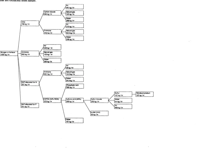
The natural resource consumption associated with industrial processes is often shown with supply chain maps or chemical source trees. Figure 3 shows the supply chain for N, P, and K fertilizers. The resources used are natural gas, water, air, sulfur (petroleum product), phosphate rock, sylvinite ore, and seawater. Figure 4 shows the source tree for nitrogen. The natural resource consumption for each chemical is shown in Table 4. In each case, nonreactive chemical inputs are excluded. Notably, in Table 4 and Figure 4, petroleum product and natural gas use for energy production are excluded. These are included in the full life-cycle inventory data presented later. Large quantities of water used for extraction of ore and cooling purposes are excluded from all of the calculations, as these are returned to the environment.

Table 4. Natural resources used to create 1000 kg of N, P2O5, and K20 in fertilizer

Natural resource consumption for nitrogen content in

1

fertilizer, kg

I I I

Air Natural gas Water

Petroleum product (sulhr) Phos~hate rock

N

2,107

Brine (sea water) Sylvanite rock

358 9 84 107 3 60

828 4,180

p205

3,116

52

897 467 1,563

Figure 4. The raw material source tree for nitrogen fertilizer shows resource use per 1000 kg of nitrogen produced. The shaded boxes represent natural resources that are extracted from nature.

Natural gas 120 kg1 hr

26Q kg 1 hr Ckea

798 kg / hr Air

373 kg 1 hr

Natural gas 92.6 kg I hr

Water 208 kg I hr

*

cr

AMMONIA AIR EMISSION FROM THE BARV

The quantity of ammonia air emissions from the barn is thought to be a function of the nitrogen content in the feed, efficiency of the animal in utilizing nitrogen, animal species and condition, housing type and waste management system, and environmental

conditions in the building (Arogo et al. 2001). Because of the large number of pertinent parameters, we might expect a wide variety of emissions being reported. In this study, we compare data from both secondary sources (reported values without detailed

information) and primary sources, which contain detailed experimental results. The primary sources were examined in much greater detail to understand the applicability of the experiments, and how these should compare to other experiments.

In order to compare the emissions data, a common unit is needed. This emission unit is the percent loss of the input waste. In this case, the input waste is the raw waste from the pig. Emissions have often been reported using bases of emissions per pig, per pig place, and per kg of live weight. In order to convert these emission measurements into an emission factor (percent loss of N excreted from the animal), we assume that the emissions are linearly related to live weight and that the waste mass and composition produced per unit of live weight is constant. The details of these calculations are shown in Appendix C.

The bases of emissions per pig or per pig place have been used, because emissions are fundamentally related to the area of the emitting surface. Between 25% and 75% of the emissions in a pit system originate from the pit (Aarnink and Wagemans 1997), while the remainder comes from the fouled portion of the floor. The pit area is most closely related to pig places and the fouled area of the floor is a function of the pig weight, number of pigs, and pig activity. Because emissions are a function of each parameter, no basis has become standard. However, live weight and number of pigs are both related to barn size through design principles, especially within a given country or region. Therefore, the selection of units is not critical when averaging results over many studies.

On any given farm, we can expect that the emissions would vary based on the type of feed used, the types of pigs being raised, the type of waste management system employed, and the cleaning schedule for the barn. However, the averages from the literature will give a good indication of the total emissions for a wider group of farms in a given area. Therefore, this information provides guidance in determining public policy or good management guidelines.

Experimental techniques for determining ammonia emissions from the barn typically require measuring gas flow rates out of the building concurrent with ammonia concentration levels near the ventilation fans. Ideal 1 y, the background ammonia concentration around the building should be measured and subtracted from the interior concentration (the flow rates out of and into the barn will be equal). In some studies, the ammonia concentration is measured outside the barns and compared to the concentration '

Experimental time frames range from days to several months. The shorter period

, measurements obviously require extrapolation to obtain a yearly emission and an

emission factor (percent loss). This requires one to assume that the time period of the sampling spanned an entire day and accurately represented yearly average conditions. When these conditions were not met, the data were adjusted.

Ammonia emissions vary over the course of a day due to temperature fluctuations and changes in pig activity. Several experiments have quantified increased emissions during the day and/or after feedings (Burton and Beauchamp 1986; Aamink et al. 1995; Aamink et al. 1996; Aamink and Wagemans 1997; Demmers et al. 1999; Harper et al. 2004b). Seasonal fluctuations are also expected. Emission measurements are typically higher in the summer months. This is probably due to a combination of higher vapor pressure and greater fan use for cooling requirements. Many researchers have noted that

measurements made during the summer months are often higher than other seasons or represent a maximum estimate of emissions.

Several papers have presented emissions by season or by month. Another subset of papers has included graphs of diurnal emission patterns. Data on both seasonal and diurnal patterns are summarized in Appendix C, and correction factors are calculated for seasonal emissions and for daytime or nighttime emissions.

.4 comparison of the literature data is shown in Table 5. Seasonal data and time of day are tabulated as well as the date of original publication and region (Europe or the United States). The calculated emission as a percentage of excreted TKN is shown as well as the emission corrected for season and time of day.

Table 5. Emission factors for nitrogen loss in the barn and storage facility

I T . 1 . 1 . . .

...

. .I 1

Hartun and Philli s (1 994)

1

1

No dateshimes

1

No dates van der Eerden et al. (1 98 1 )

Kowalewsky (198 1) Burton and Beauchamp

( 1 986)

17.4

Whole year 16.2 I No dates1

1 times 21.0 Gustafsson (1 987)

Grassland Research institute

17.4

Kruse et a]. (1989)

1

Aarnink et a]. (1995)

1

Oldenburn ( 1989)

198 1

times

1

15.4

E

times 21.1 Hoeksma et a]. (1 993)

I Groenestein (I 993) and

I Montsma and Groenestein

(1 992)

Aarnink et al. (1 995) times

No dates/ times

I Whole year Groenestein and van Faassen

1

11 996) Winter

1

1 12.1

1

19.5

1

1996

1

E

I

Most of year

1

9.6

1

9.6

1

1996 ( E Aarnink, et a]. (1996)

Summer and

winter

(

14.9 Winter and

Aarnink, et al. (1997) Aarnink and Wagemans

( 1997) early summer

1

1 1.5

Arogo et al. (200 1) Demmers et al. ( 1999)

Hendriks et a]. (1998)

I

~i et al. (2000a)

No datedtimes Summer & fall

Harris et al. (2001)

23.6 32.0

Heber et al. (200 1 )

Summer No dates/ times No dates/ Arogo et al. (2001)

1

Pahl et al. (2002)

E

E 23.6 -

23.2

31.2

3.8

times 118.5

/

18.5 12002 I E

1

1998 - 1998

22.6

3.8

Harris and Thompson (1 998)

2001

2001

L I

Studies prior to the early 1990s generally have lower estimates of percent nitrogen lost than more recent studies.

Table continued

* E=Europe, US=United States

f

0 0 - g g _*

5.E

$ + k g 2

S U E " % 22.7

22.5 17.2 17.7 7.4

L

.E

G S

o m

22.7 22.5 17.4 16.9 5.6 16.9 17.0 X

a -0

c,

u

.- E T

G

Whole year Whole year w

2

3

z

i?

(d E .

-

& Van der Hoek (1 998)

Misselbrook et al. (2000)

-

.

E

1978 2000

Median Mean

Standard deviation Mean of European data Mean of US data

w

2

I

Sf

2

m

c

3

.

m

*

E

0

2

NITROGEN LOSSES IN LAND APPLICATION

Nitrogen, phosphorus, potassium. and carbon are all emitted during and after land application of swine waste. Nitrogen is emitted into the air in the form of ammonia (NH3), nitrous oxide (N20), and nitrogen oxides (NO,). Nitrogen, phosphorus, and potassium move into the soil. Previous life-cycle assessments have ignored the effects of leaching from farmland. This is due to both a lack of knowledge about the assessment and migration of these chemical emissions and a lack of actual emission data. Leaching emissions are not included in this life-cycle report. Carbon is emitted to the air in the form of carbon monoxide, carbon dioxide, and methane. All of these carbon-based chemicals have global warming potential. However, relative to nitrogen, there are little data on these emissions. Furthermore, there is a large background flux of carbon into and out of the soil due to natural processes. Therefore, carbon emissions are also ignored in this study.

Here, we focus on nitrogen emissions to the air. Specifically, we tabulate values for NH3

and NzO emissions during and after the application of swine waste. These chemicals are also emitted naturally without any fertilizer or waste application. Therefore, experiments typically include measurements on a control plot. The values shown in this study have the emissions from the control subtracted when these are given.

Ammonia and N 2 0 are also emitted when commercial fertilizers are applied. Although we chose not to subtract these emissions (as avoided emissions), these may be

comparable to those from animal waste. In fact, Mosier et al. (1 996; 1998) assume that application of synthetic or manure N contribute equally to N 2 0 emissions.

Bouwman (1 996) estimates that 1.25% of applied N is emitted as N 2 0 over > 100 days. Bouwman et al. (2002a) showed that emissions of N 2 0 depend on application rate, fertilizer type (chemical form of N), and crop type. They studied 846 emission

measurements in the literature and found that the chemical form of the fertilizer could affect emissions by a factor of 3, but that application method did not have a significant effect. Using a model based on these 846 emission measurements, Bouwrnan et al. ( 2 0 0 2 ~ ) calculated that world average emissions for animal manure were 0.8% and world average emissions for commercial fertilizer were 0.9%. Bouwman et al. ( 2 0 0 2 ~ ) and Mosier et al. (1998) showed that the N 2 0 emission factor increases as the application rate increases. Therefore, if a farmer were to apply effluent in addition to commercial fertilizer, the emissions would likely be greater than those used in this life-cycle study. Ammonia emissions from synthetic fertilizer are also significant. Bouwman et

al. (2002b) studied data from 1,900 NH3 volatilization measurements in the literature. They estimate that in industrialized countries, 7% and 2 1% of the N from application of synthetic fertilizer and animal manure, respectively, is volatilized as NH3. Globally the volatilization rates are 14% and 23% for fertilizer and manure. The NH3 emissions in industrial countries are lower because of the use of different chemicals and application methods as well as a different average climate.

During the application process, the spreading methods have lower aerosolization and ammonia volatilization than irrigation, due to a relatively short throw from the applicator to the ground. Surface spreading methods include band spreading (applying in narrow bands to reduce volatilization area) and broadcasting (distributing over the entire

surface). Injection or subsurface methods require either directly injecting the manure into the soil or incorporating it soon after spreading onto the surface (harrowing). The

injection methods lead to the lowest ammonia volatilization rate.

Ammonia and nitrous oxide emission rates defined as a percent loss (of applied TKN and applied total ammonia nitrogen, TAN) are estimated for effluent irrigation, for surface spreading, and for injection of sludge. In the life-cycle inventories, we assume that all of the lagoon liquid is irrigated, and that the sludge is either surface applied or injected. Losses of NH3-N during and after irrigation that are reported in the literature have ranged from 10% to 99% when animal waste is surface applied (Vanderholm 1975). Several authors have suggested that about 50% of the TKN that is irrigated is available for plants (Westerman et al. 1995; Al-Kaisi and Waskom 2002). Numerous factors such as manure pH, soil pH, soil and atmospheric temperature (seasonal), soil type, crop type, application method, and wind speed are thought to determine the amount of nitrogen loss.

Hoff et al. (1 98 1) suggest that acidity (pH) of the soil and manure as well as application method are the primary indicators of ammonia volatilization. Acidity decreases

volatilization by lowering the NH3 to N H ~ ' ratio. The importance of pH indicates that TAN may be important as well. We explore the effect of both application method and TAN application rate on ammonia volatilization. Application methods are categorized as irrigation, surface spreading, and injection. We also test the effect of application rate on emissions when measured as a percent loss. The spreading and injection experiments (in the literature) on emissions have been performed using raw waste. Lagoon sludge has a much lower ratio of TAN:TKN ( f') than manure and presumably lower volatilization rates. We extrapolate the data to determine the emissions at an average f' value for lagoon sludge.

NITROGEN LOSSES FROM LAGOON EFFLUENT APPLICATION

Lagoon effluent is typically spray applied (irrigated) with a sprinkler system or 'big gun.' Several researchers have measured the ammonia volatilization during irrigation. The concentration and flow rate leaving the irrigator is measured and compared to the

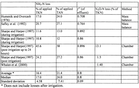
concentration and flux of ammonia that reaches the surface, as measured with collection devices. Typically 10%-20% is lost during irrigation. Table 6 shows results for each research paper.

Table 6. Nitrogen loss during irrigation of lagoon emuent

- --

Humenik and Overcash (1 976)

Safley et al. (1 992)

Sharpe and Harper (1 997) (during irrigation)

Sharpe and Harper (1 997) (during irrigation)

Sharpe and Harper(l997) (post irrigation up to 24 hours)

Sharpe and Harper( 1997) (post irrigation)

Whalen et al. (2000)

f' (of

0.708

balance

0.764 Mass

NH3-N loss

Average

*

Median

Standard deviation

% of applied TKN 17.0

20.7

1 1.6

1 0.8

45.6

24.2

0.896 Chamber

% of applied TAN 24.0

27.1

0.892 13.0

12

58

27.2

16.4 17.0 4.58

- -

*

Does not include losses after irrigation.

Each entry represents an average of the experiments presented in each publication. balance

21.4 24.0 7.4 1

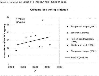
The effect of soil pH is not relevant in determining the ammonia losses during irrigation, and the pH of the effluent was not given for each experiment. However, the ratio o f TAN to TKN or

/' value was given and is shown to be significant. A regression plot is shown

in Figure 5. We assume that the relationship is linear over the full range of 0 5

f c

5 1

.

All of the volatilization is assumed to be from ammonia; therefore, the intercept is forced through zero. An analysis performed with StatView shows a slope of 18.7% losslunit f'

and a standard error (66% confidence interval) of 2.5% losslunit f'. Although the R~ value for fit that is forced through zero is 0.88, it is clear that other factors affect the measured loss. Over the f' range of the experiments, percent losses vary from 13% to

Figure 5. Nitrogen loss versus j"' (TAN:TKN ratio) during irrigation

Ammonia loss during irrigation

! a Sharpe and Harper (1 997)

I /

I A Safley et a1. (1 992) i 0 Humenik and Overcash i

(1 976)

I

I x Westerm an et at. (1 995)

I - I

t

I

-

Sharpe and Harper (2002)

I

I

1

-linear fit ( ~ 1 8 . 7 ~ )

I

I

, The linear fit, which is forced through zero, has a slope o f 18.7 and a standard error of 2.5.

assumption that postirrigation emissions are similar to surface application emissions from raw waste (corrected for ammonia content). The value is significantly smaller than Sharpe and Harper (1997) but close to Sharpe and Harper (2002).

The industrial fertilizer emission replacement credits are based on the N, P, and K available to crops. Therefore, in the context of this report, higher N losses during land application would increase both indirect (more N fertilizer manufacturing) and direct emissions. If the NH3 emissions estimate for land application were revised upward, the incentive for conserving N in the storage/processing step would be reduced. As a result, the environmental improvements yielded from utilizing an alternative to the anaerobic lagoon would be diminished.

NITROGEN LOSSES FROM SURFACE APPLICATION

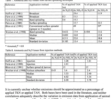
Several methods are available for application of slurries or solids. These can be categorized as surface spreading or injection methods. Ammonia and N 2 0 loss values From the literature are given in Table 7 (for surface application) and in

*

Assumed f = 0.8

Table 8. Ammonia and N 2 0 losses fiom injection methods.

Table 7. Ammonia and N 2 0 losses from surface spreading techniques

Hoff et al. (1 981)

Ferm et al. (1 999)

Bless et al. ( 1 99 1) Weslien et al. (1 998)

A ~ ~ l i c a t i o n method

Injection

* Assumed f = 0.8

,

Reference

Hoff et al. (1 98 1)

Ferm et al. (1 999)

Ferm et al. (1 999)

Pain et al. ( 1 989)

Bless et al. (1 99 1)

Weslien et al. (1 998)

b

% of applied TKN lost

Injection

Surface spread & harrow Various subsurface Median Application method Broadcast Broadcast Band spreading Surface spreading

Conventional surface spreader (sprayer w/ 5 nozzles)

Band spreading Median Mean

Standard deviation

% of applied TAN lost

AS N20-N

0.504

% of applied TAN lost % of applied TKN lost AS N20-N AS NH3-N AS N20-N AS NH3-N

3.26 1.61

AS N20-N

0.3 0.6 0.632 0.600 0.51 1 0.183

AS NH3-N

11.9 10.5 39* 13.6 12.8 18.8 13.6 AS NH3-N 19.4 15.5 14.3 15.7 49 17.9 16.8 22.0 13.4

It is currently unclear whether emissions should be approximated as a percentage of applied TKN or applied TAN. Both bases have been used in the literature, and neither correlations adequately describe the variation in emission data from application of animal

manure. Bowwman and Van der Hoek (1 997) showed that the chemical form of N is

important.

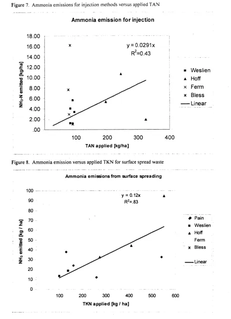
We plot NH3 emissions from surface spreading and injection versus both TKN and TAN. The importance of ammonia concentration is then tested using a plot of emissions (as a percent of TKN) versus f'

.

The intercept of each regression is forced through zero. Doing so inherently assumes that emissions are zero when the tested parameter (TKN, TAN, f e ) is zero. This is necessarily true for plots versus TKN. However, the

assumption is not as clear for plots versus NH3 and f'

,

because organic nitrogen can be converted to ammonia in the soil. The R* values reported apply to the constrained fit (no intercept), and are generally higher then the values for an unconstrained fit.

5.34 5.78

Mean

Standard deviation

Figure 6 and Figure 7 show emissions versus TAN with linear regressions, which have the intercept forced through zero. The regressions give emissions of 0.164 kg NH3/kg NH3 applied for surface spreading methods and 0.029 kg NH3/kg NH3 applied for

injection methods. These emission coefficients have standard errors of 0.022 and 0.01 or 6.02

13% and 34%, respectively. The R~ values (0.70 and 0.43) confirm that other variables are significant.

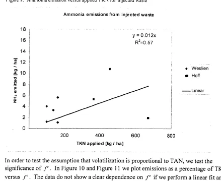
Of the emissions data included here, less information on TKN applied (as compared to TAN applied) was available. The emissions are plotted versus TKN application rate along with linear regressions in Figure 8 and Figure 9. Nine data points for surface spreading give a loss rate of 0.12 kg NH3-Nikg TKN applied, when the linear regression is forced through zero. The standard error in the slope is 0.019 (16%), and the R* value was 0.83. For injection methods, eight data points yield a loss rate of 0.012 kg NH3-N/kg TKN applied. The standard error of the slope was 0.004 (33%), and the R~ value was

0.57.

Figure 6. Ammonia emissions for surface application methods versus applied total ammoniacal nitrogen

(TAN)

Ammonia emission for surface spreading

i

I Pain

A Weslien Hoff

A Ferm Bless

-

- Linear .-.

100 200 300 400

Figure 7. Ammonia emissions for injection methods versus applied TAN - - - -- - . . - - - ..

Ammonia emission for injection

Weslien

A Hoff x Ferm x Bless

-

_{- - - -} Linear _{- - - - -}

100 200 300 400

TAN applied [kglha]

- - - . - . . . - - - - . - -

Figure 8. Ammonia emission versus applied TKN for surface spread waste

--_ _ . - . _ _ - - _ _ _ _ _ - _ - . - - - - - . - - - . -

Ammonia emissions from surface spreading

- - - - . . . -

Pain Weslien A Hoff

Ferm

' x Bless

-

Linear

Figure 9. Ammonia emission versus applied T K N for injected waste

Ammonia emissions from injected waste

I - -

I + Weslien

Hoff

-

Linear

- -- - . - . - - -

200 400 600 800

TKN applied [kg I ha]

In order to test the assumption that volatilization is proportional to TAN, we test the significance of /'

.

In Figure 10 and Figure 1 1 we plot emissions as a percentage of TKN versus f'

.

The data do not show a clear dependence on

P

if we perform a linear fit and do not restrict the emissions at f' = 0 . The unrestricted linear fit (not shown) for

broadcasting (surface spreading) is strongly influenced by one data point (30% loss) from Pain et al. (1989) and has a large intercept and negative slope. The fit for injection has a reasonable intercept (-0.5) and slope (3.9), but the standard error in the slope is 3.7. We assume that any conversion from organic N to TAN on the soil surface is negligible. This forces the fit through zero and yields lower standard errors. Figure 10 and Figure 1 1 show the data with linear regressions that were forced through zero. For surface

Figure 10. A linear regression, which is forced through zero is fit to ammonia emissions from surface

spreading.

Ammonia emissions from surface spreading

B Pain !

A Weslien Hoff L i n e a r

Figure I I . Ammonia emissions from injection application are shown with a linear regression that is forced through zero.

- - .

Ammonia emissions from injection

A Hoff

0 Weslien

-

Linear

The linear regressions in Figure 10 and Figure 1 1 are used to predict the ammonia volatilization losses at average f' values. The f' values for raw waste and surface spreading studies are shown in Table 9. The f' values of raw waste from the barn are very near to the f' values used in surface application studies in the literature. The median value of f' for the composite data is 0.64. The

f

values for sludge from

anaerobic lagoons are shown in Table 10. Because most of the TAN leaves the lagoon in the effluent phase, the average f e of sludge value is considerably lower (0.26) than that of raw waste. Therefore, the emissions from sludge application should be significantly lower than emissions from raw waste application.

Table 9. TAN:TKN ratio from raw waste and surface spreading studies

. - - - . - . - . I/

(f' of-raw waste, Barker

]

j' from surface spreading

I

(2002)

0.582 0.479

studies Reference Pain et al. (1989) Pain et al. (1 989)

f' value

1

Table continued

10.347 lweslien et al. (1998) 10.556

1

0.930

0.828 0.847 0.872

10.69 1

1

Weslien et al. (1 998) 10.556

1

0.658 0.442 0.830 0.696 0.612 0.410 0.490 0.740 0.426 0.480

Pain et al. (1989) Pain et al. (1989) Weslien et al. (1 998) Weslien et al. (1 998) Hoffetal.(1981) Hoff et al. (1981) Hoff et al. (1981) Hoffetak(1981) HoffetaL(1981) 0.619 0.534 0.535 0.484 - 0.676

Table 10. The f" value for lagoon sludge. Data from Bicudo et al. (1 999) is from 15 separate lagoons in 0.629

0.628 0.1 94

North Carolina.

Weslien et al. (1998) Weslien et al. (1998) Weslien et al. (1998)

0.696 0.830 0.830 Median Mean Standard deviation 0.638 0.642 0.122

Bicudo et al. (1999) Bicudo et al. (1999)

I

Bicudo et al. (1999)

I

2400

1

600

1

0.250

1

Bicudo et al. (1999)

Bicudo et al. (1999)

TKN [mg/l]

2800 3300 3200 3400

Bicudo et al. (1999) Bicudo et al. (1999)

~ i c u d o et al. (1 999)

I I I

4200

1

1000

1

0.238

1

NH3-N

500 600

Bicudo et al. (1999) Bicudo et al. (1 999)

>

f "

0.179 0.182 500 500 1200 6200 0.156 0.147 4200 4500

Bicudo et al. (1999) Bicudo et al. (1999) Bicudo et al. (1999) Bicudo et al. (1999) Bicudo et al. (1 999)

Humenik and Overcash (1 976) ,

Humenik and Overcash(1976) Humeni k and Overcash( 1 976) Humenik and Overcash (1 976)

500 700

Hurnenik and Overcash (1 976)

0.417 0.113 1000 1 100 3 200 3300 5 800 5700 4200 3300 3570 3600 3500, 0.238 0.244 3900 Mean Standard deviation Median 800 1100 1500 1500 1000 990 1060 1230 1620,

It is unclear whether emissions should be based on an average value from each literature source, a regression of emissions versus TKN, or a regression of data versus TAN. Therefore, emissions calculated for each of these methods are tabulated in Table 1 1. The literature averages weight each surveyed paper evenly. The values based on regression weights each experiment presented in the papers evenly and uses the dependence on f c to predict the loss for sludge.

Table 11. Summary of ammonia volatilization losses during land application

I

NH3-N loss [% of TKN]

I

Irrigation of lagoon effluent

Postirrigation losses of lagoon effluent Surface application of raw waste Surface application of lagoon sludge Injection of raw waste

Injection of lagoon sludge

*The loss rate for irrigation refers to losses before contact with the land surface.

**

Post irrigation losses are estimated using the surface application correlation. The total loss rate from Median of

literature

1 1.6*

12.8

12.8

2.4

2.4

irrigation and subsequent volatilization is 29%.

NITROUS OXIDE EMISSIONS DURJNG LAND APPLICATION Loss based on

regression (vs.

f)

15.6**

The physical mechanisms of nitrous oxide emissions are more complicated than those of ammonia emissions. Nitrous oxide is formed through both nitrification and

denitrification. Both of these processes are sensitive to the environment, which can contribute to a high variability in emissions. Specifically, the oxygen concentration and rainfall can greatly impact N 2 0 emissions. Due to the more complicated chemistry involved, it is quite possible that N 2 0 emissions are not directly proportional to the amount of TKN or TAN applied, but are strongly influenced by other processes.

In addition to direct emissions, which can be measured, ammonia emissions and leaching can contribute to nitrous oxide emissions elsewhere (Mosier et al. 1996; Mosier et al.

1998). Weslien et al. (1998) estimate that the secondary emissions due to nitrate leaching

are comparable to the direct emissions. In this report, we consider only direct

atmospheric emissions. We tabulate the reported emissions (as percentages of applied TKN) in the literature. Several studies considered land application and several

considered irrigation. Although the irrigation studies have higher emission values, there Loss based on

regression (vs. TAN applied)

15.9*

10.5

4.2

1.8

0.076

Loss based on regression (vs. TKN applied)

12.0

1.2

f

0.8

0.85

0.64

0.26

0.64

are not enough data to justify using separate emission factors; therefore, we consider these together.

. In Table 12, N 2 0 losses are tabulated with equal weight for each researcher. With the

exception of Sharpe and Harper (1 997), the losses range from 0.4% to 1.5% of the applied TKN. The mean is not included in the table, because it is largely influenced by the data from one study (Sharpe and Harper 1997). The median value (1.4%) is used in the life-cycle study. This value is comparable to other studies on N 2 0 emissions after applying chemical fertilizer and/or animal manure (Cates and Keeney 1987; Eichner

1990; Bouwman 1996; Bouwman et al. 2002~). Table 12. Summary of N 2 0 emissions during land application

Whalen et al. (2000)

Weslien et al. (1 998)

Rochette et al. (2000)

Ferm et a]. (1999)

N20-N loss

[% of TKN applied]

Sharpe and Harper (1 997) Sharpe and Harper (2002)

Median

We calculate the value for

N20-N loss

[% of NH3-N applied] Author Application

loss as a percentage of applied TKN for Ferrn et al. (1999) by assuming that Irrigation

Surface and i~jection methods

Surface Irrigation Irrigation

fe=0.8. The mean is strongly affected by the value given by Sharpe and Harper (1997), and not enough data are available to determine, based on the standard deviation, if this is an outlier.

0.36 13.00

LAND APPLICATION EMISSIONS USED IN THE LIFE-CYCLE CALCULATIONS 1.400 0.400 1.450 0.288 10,400 1 SO0 1.430

Table 13 contains the land application emissions that were used in the life-cycle inventory calculations. Carbon volatilization, N2 volatilization due to nitrification denitrification cycles, and leaching of the primary nutrients are neglected.

Table 13. Land application losses used in the life-cycle inventory

% of applied TKN lost to NH3-N volatilization

Irrigation

Surface spreading of solids Injection of solids

% of applied TKN lost to N20-N volatilization

29 12

2.4

ANAEROBIC LAGOON

When swine waste enters the anaerobic lagoon, a portion of it becomes dissolved or suspended in the supernatant or liquid phase, and another ponion settles to the bottom, which is often designated the sludge phase. This process is quick; however, there is a time-dependent redistribution of material from one phase to the other over the life span of the lagoon. A portion of the organic carbon material in the sludge is stabilized as

anaerobic biomass, and the rest is broken down to form biogas ( C 0 2 and CH4). Several of the organic nitrogen-containing compounds are stabilized, while the rest are broken down into ammonia. For the life-cycle inventory, we are concerned with the quantity of nitrogen, potassium, and phosphorus left in the sludge and supernatant phases when these are removed and land applied. We are also interested in the mass flux of ammonia and biogas from the lagoon. Ammonia contributes to acidification and eutrophication, and the biogas contributes to global warming potential.

The general model for nutrient tracking and emissions is shown in Figure 12. A small percentage of potassium and phosphorus is lost to seepage, and the rest is split between the effluent and sludge. This seepage is only a calculation based on water loss and concentration of chemical species and not a verification of significant movement be1 the bottom soil layer. Nitrogen is lost primarily through seepage, evaporation of ammonia, and possibly evaporation of dinitrogen (Harper et al. 2000; Harper et al. 2004a). Volatile solids are not conserved, and the carbon content is not tracked. However, carbon dioxide and methane emissions are related to volatile solids remov To estimate C 0 2 and CH4 emissions, we use an average gas production per unit live weight from the literature.

Figure 12. Mass transfer model o f anaerobic lagoon

NH,-N

evaporated

VS in effluent

1

P in waste P in sludge (50%)

P lost to seepage (2%)

K in effluent (87%)

rC--7

K ~n waste K in sludge (5%)

VS converted to CO,

(0 83 g CO, 1 kg LW)