University of Windsor University of Windsor
Scholarship at UWindsor
Scholarship at UWindsor
Electronic Theses and Dissertations Theses, Dissertations, and Major Papers
2010
Application of electrical methods to assess the quality of
Application of electrical methods to assess the quality of
concrete
concrete
William Clements University of Windsor
Follow this and additional works at: https://scholar.uwindsor.ca/etd
Recommended Citation Recommended Citation
Clements, William, "Application of electrical methods to assess the quality of concrete" (2010). Electronic Theses and Dissertations. 7975.
https://scholar.uwindsor.ca/etd/7975
This online database contains the full-text of PhD dissertations and Masters’ theses of University of Windsor students from 1954 forward. These documents are made available for personal study and research purposes only, in accordance with the Canadian Copyright Act and the Creative Commons license—CC BY-NC-ND (Attribution, Non-Commercial, No Derivative Works). Under this license, works must always be attributed to the copyright holder (original author), cannot be used for any commercial purposes, and may not be altered. Any other use would require the permission of the copyright holder. Students may inquire about withdrawing their dissertation and/or thesis from this database. For additional inquiries, please contact the repository administrator via email
APPLICATION OF ELECTRICAL METHODS
TO ASSESS THE QUALITY OF CONCRETE
by
William Clements
A Thesis
Submitted to the Faculty of Graduate Studies
Through the Department of Civil and Environmental Engineering
in Partial Fulfillment of the Requirements for
the Degree of Master of Applied Science at the
University of Windsor
Windsor, Ontario, Canada
2010
1*1
Library and Archives CanadaPublished Heritage Branch
395 Wellington Street Ottawa ON K1A 0N4 Canada
Bibliotheque et Archives Canada
Direction du
Patrimoine de I'edition
395, rue Wellington Ottawa ON K1A 0N4 Canada
Your file Votre reference ISBN: 978-0-494-62739-6 Our file Notre rdf6rence ISBN: 978-0-494-62739-6
NOTICE:
The author has granted a
non-exclusive license allowing Library and Archives Canada to reproduce, publish, archive, preserve, conserve, communicate to the public by
telecommunication or on the Internet, loan, distribute and sell theses
worldwide, for commercial or non-commercial purposes, in microform, paper, electronic and/or any other formats.
AVIS:
L'auteur a accorde une licence non exclusive permettant a la Bibliotheque et Archives Canada de reproduire, publier, archiver, sauvegarder, conserver, transmettre au public par telecommunication ou par I'lnternet, pr§ter, distribuer et vendre des theses partout dans le monde, a des fins commerciales ou autres, sur support microforme, papier, electronique et/ou autres formats.
The author retains copyright ownership and moral rights in this thesis. Neither the thesis nor substantial extracts from it may be printed or otherwise reproduced without the author's permission.
L'auteur conserve la propriete du droit d'auteur et des droits moraux qui protege cette these. Ni la these ni des extraits substantiels de celle-ci ne doivent etre imprimes ou autrement
reproduits sans son autorisation.
In compliance with the Canadian Privacy Act some supporting forms may have been removed from this thesis.
Conformement a la loi canadienne sur la protection de la vie privee, quelques
formulaires secondaires ont ete enleves de cette these.
While these forms may be included in the document page count, their removal does not represent any loss of content from the thesis.
Bien que ces formulaires aient inclus dans la pagination, il n'y aura aucun contenu manquant.
• + •
Author's Declaration of Originality
I hereby certify that I am the sole author of this thesis and that no part of this
thesis has been published or submitted for publication.
I certify that, to the best of my knowledge, my thesis does not infringe upon
anyone's copyright nor violate any proprietary rights and that any ideas, techniques,
quotations, or any other material from the work of other people included in my thesis,
published or otherwise, are fully acknowledged in accordance with the standard
referencing practices. Furthermore, to the extent that I have included copyrighted
material that surpasses the bounds of fair dealing within the meaning of the Canada
Copyright Act, I certify that I have obtained a written permission from the copyright
owner(s) to include such material(s) in my thesis and have included copies of such
copyright clearances to my appendix.
I declare that this is a true copy of my thesis, including any final revisions, as
approved by my thesis committee and the Graduate Studies office, and that this thesis has
ABSTRACT
The desire for a non-destructive testing method for concrete strength has always been
present in civil engineering. An emphasis on testing the electrical properties of concrete
has existed for many years without the connection drawn between the electrical
properties and strength of concrete. This study was designed to determine if a relationship
between the electrical properties and strength of concrete exists. It was found that a linear
relationship exists between the capacitive reactance and strength of concrete, as concrete
cures and sets. It was also found that increasing the electrode distance increases the
reactance, increasing the electrode contact area decreases the reactance and decreasing
DEDICATION
I would like to dedicate this thesis to Diana, because without her help, understanding and
ACKNOWLEDGEMENTS
I would like to thank Dr. S. Das and Dr. G. Raju for accepting me as a MASc student and
for all of their help along the way. I would like to thank Dr. S. Das for always pushing me
and making sure I was on track, and for helping me throughout the writing process. I
would like to thank Dr. G. Raju for sharing his knowledge and experience with electrical
engineering with me as it was very helpful in the completion of this project.
I would like to thank the Civil Engineering technicians Lucian Pop and Matt St. Louis for
all their help with this project. Whether it was putting up with my testing in their lab or
helping create the specimens for testing I would like to thank both of you. I would also
like to thank my colleague Thomas Ring for helping me learn some of the testing
equipment early on in my experimental program.
I would also like to thank my family for all of the support during this process, and I will
be happy to say I am finally finished school.
Lastly, I would like to thank Diana a final time as she sacrificed the most in order to see
me complete this project. Whether it was bearing with me as I completed electrical
readings on the weekends, losing some time together or helping with anything she could I
TABLE OF CONTENTS
AUTHOR'S DECLARATION OF ORIGINALITY iii
ABSTRACT iv
DEDICATION v
ACKNOWLEDGEMENTS vi
LIST OF TABLES xii
LIST OF FIGURES xiii
1 INTRODUCTION 1
1.1 GENERAL 1
1.2 PROBLEM STATEMENT 1
1.3 OBJECTIVE 1
1.4 SCOPE OF WORK 2
1.5 METHODOLOGY ...2
1.6 SCOPE OF WORK 2
2 LITERATURE REVIEW 3
2.1 GENERAL 3
2.2 CEMENT PASTE 3
2.2.1 RELATIONSHIPS BETWEEN ELECTRICAL AND PHYSICAL
PROPERTIES OF CEMENT PASTES 3
2.2.2 EFFECT OF WATER CONTENT IN CEMENT PASTES 6
2.2.4 EFFECT OF WATER TYPE ON CEMENT
PASTES 9
2.3 MORTAR 12
2.3.1 EFFECT OF WATER CONTENT ON THE ELECTRICAL
IMPEDANCE OF MORTAR 12
2.4 CONCRETE 17
2.4.1 ELECTRICAL RESISTIVITY OF CONCRETE 17
2.4.2 DIELECTRIC PROPERTIES OF CONCRETE 21
2.4.3 RELATIONSHIP BETWEEN RESISTIVITY AND STRENGTH
OF CONCRETE 26
2.4.4 VARIATION OF ELECTRICAL PROPERTIES OF CONCRETE
WITH FREQUENCY 28
2.4.5 EFFECT OF CEMENT TYPE ON THE IMPEDANCE OF
CONCRETE 32
2.4.6 ELECTRICAL PROPERTIES OF CONCRETE AND CONCRETE
CONSTITUENTS 36
2.4.7 DETERMINATION OF CONCRETE SETTING TIME 37
2.5 SUMMARY 39
3 EXPERIMENTAL PROGRAM 40
3.1 CONCRETE MATERIALS 40
3.2 CONCRETE AND CEMENT PASTE MIXES 43
3.4 TEST MATRIX 52
3.5 SPECIMENS USED FOR PHYSICAL PROPERTIES OF
CONCRETE 54
3.5.1 MIXING LARGE CONCRETE SAMPLES 54
3.5.2 SLUMP TEST 54
3.5.3 CONCRETE COMPRESSION TEST 55
3.5.4 CONCRETE DENSITY 58
3.6 SPECIMENS USED FOR ELECTRICAL PROPERTIES OF
CONCRETE 59
3.6.1 CASTING CONCRETE FOR ELECTRICAL
MEASUREMENTS 59
3.6.2 ELECTRICAL DATA ACQUISITION 61
4 CIRCUIT REPRESENTATION 63
4.1 GENERAL 63
4.2 SERIES CIRCUIT 63
4.3 PARALLEL CIRCUIT 68
4.4 PARALLEL CIRCUIT IN SERIES WITH A RESISTOR 71
4.5 SUMMARY 73
5 EXPERIMENTAL RESULTS 74
5.1 INTRODUCTION 74
5.2 PHASE I RESULTS 74
5.2.2 COMPRESSION STRENGTH 74
5.2.3 ELECTRICAL TESTING RESULTS 77
5.2.4 ANALYSIS OF PHASE I RESULTS 81
5.3 PHASE II RESULTS 83
5.3.1 ELECTRICAL TESTING RESULTS 83
5.3.2 ANALYSIS OF PHASE II RESULTS 84
5.4 PHASE III RESULTS 85
5.4.1 SLUMP AND DENSITY 85
5.4.2 COMPRESSION STRENGTH 86
5.4.3 ELECTRICAL TESTING RESULTS 89
5.4.3 ANALYSIS OF PHASE III RESULTS 92
5.5 PARAMETRIC STUDY 94
5.5.1 EFFECT OF ELECTRODE SPACING 94
5.5.2 EFFECT OF ELECTRODE CONTACT AREA 96
5.5.3 EFFECT OF CEMENT CONTENT 98
5.6 SUMMARY 100
6 SUMMARY, CONCLUSIONS, AND RECOMMENDATIONS 102
6.1 SUMMARY 102
6.2 CONCLUSIONS 103
6.3 RECOMMENDATIONS 104
APPENDIX B - ELECTRICAL PARAMETER PLOTS 108
APPENDIX C - STRESS-STRAIN PLOTS 110
APPENDIX D - INTRODUCTION OF DEFECT INTO CONCRETE 114
LIST OF REFERENCES 117
List of Tables
Table 3.1: Standard sieve sizes 41
Table 3.2: Grain size analysis results 42
Table 3.3: Concrete mixes of Trial 1 44
Table 3.4: Concrete mixes of Trial II 45
Table 3.5: Cement paste mixes 45
Table 3.6: Concrete mixes of Trial III 46
Table 3.7: Dimensional properties of concrete moulds 49
Table 3.8: Test matrix 52
Table 3.9: Concrete mould labelling methodology 53
Table 5.1: Density of cylinders in Phase 1 74
Table 5.2: Phase I compression strength results 76
Table 5.3: Density of cylinders in Phase III 86
Table 5.4: Phase III compression strength results 88
Table 5.5: Comparison of strength between Concrete Mix I and II 89
Table A.0.1: Average reactance for specimens tested in Phase I 99
Table A.0.2: Average reactance for specimens tested in Phase II 100
Table A.0.3: Average reactance for specimens tested in Phase III 101
List of Figures
Figure 2.1: Schematic for the conduction of electricity through cement paste
(Taylor and Arulanandan, 1974) 4
Figure 2.2: Strength of cement paste measured and calculated using b parameter
(Taylor and Arulanandan, 1974) 5
Figure 2.3: Variation of resistivity of cement pastes with the reciprocal of water content
(Tashiro et al., 1987) 6
Figure 2.4: Variation of slopes from Figure 2.3 with time (Tashiro et al., 1987) 7
Figure 2.5: Variation of resistivity with the reciprocal of water content of different
cements (Tashiro et al., 1987) 7
Figure 2.6: Pore size distribution of different cement pastes (Tashiro et al., 1987) 8
Figure 2.7: Conductivity with time using Portland cement paste (Wahed and Hekal, 1989) 10
Figure 2.8: Conductivity with time using slag cement paste (Wahed and Hekal, 1989).. 11
Figure 2.9: Conductivity with time using blended cement paste (Wahed and Hekal, 1989) 11
Figure 2.10 (a) & (b): Variation of real and imaginary capacitance with frequency
(Berg et al., 1992) 14
Figure 2.11: Complex impedance plot for mortar (Berg et al., 1992) 15
Figure 2.12: Variation of conductance with storage time (Berg et al., 1992) 16
Figure 2.13: Conduction model for concrete (Whittington et al., 1981) 18
Figure 2.14: Low frequency impedance plot of concrete (Wilson et al., 1984) 21
Figure 2.15: High frequency impedance plot of concrete (Wilson et al., 1984) 22
Figure 2.16: Variation of impedance and temperature with time (Wilson et al., 1984)... 23
Figure 2.17: Low frequency plot of resistivity and relative permittivity
Figure 2.18: High frequency plot of resistivity and relative permittivity
(Wilson et al., 1984) 25
Figure 2.19: Variation of resistivity with time (Whittington and Wilson, 1986) 27
Figure 2.20: Correlation of resistivity and strength (Whittington and Wilson, 1986) 28
Figure 2.21: Comparison of dielectric constant at one hour
(Whittington and Wilson, 1990) 30
Figure 2.22: Comparison of conductivity at one day (Whittington and Wilson, 1990)... 30
Figure 2.23: Comparison of dielectric constant at one day
(Whittington and Wilson, 1990) 31
Figure 2.24: Comparison of conductivity at one hour (Whittington and Wilson, 1990).. 31
Figure 2.25: Complex impedance plot for Portland cement (McCarter, 1996) 33
Figure 2.26: Influence of cement product used on impedance plot (McCarter, 1996) 34
Figure 2.27: Influence of using PFA on impedance plot (McCarter, 1996) 35
Figure 2.28: Effective conductivity of cement pastes
(Manchiryal and Neithalth, 2008) 38
Figure 3.1: Sand gradation results 40
Figure 3.2: Crushed stone dust used in experimental program 41
Figure 3.3: Results of sieve analysis on coarse aggregate 43
Figure 3.4: Steel cube mould 44
Figure 3.5(a): Concrete cube with face electrodes 47
Figure 3.5(b): APPA-95 multimeter 47
Figure 3.6: Concrete cube with embedded aluminum electrodes 48
Figure 3.7: Concrete Mould 1 49
Figure 3.8: Concrete Mould II 50
Figure 3.10: Scale used to measure concrete components 54
Figure 3.11: Wheel barrow used to mix concrete 54
Figure 3.12: Plastic cylinder mould 56
Figure 3.13: Filled and capped concrete cylinder 56
Figure 3.14: Applying the releasing agent 56
Figure 3.15: Setting the cylinder 56
Figure 3.16: Removing excess capping 57
Figure 3.17: Completed cylinder 57
Figure 3.18: Cylinder ready for compression testing 57
Figure 3.19: Cylinder height 59
Figure 3.20: Measuring mass of cylinder 59
Figure 3.21: Applying releasing agent to the acrylic mould 60
Figure 3.22: Eliminating voids from the concrete mould 60
Figure 3.23: Keithley 3330 LCZ meter 61
Figure 3.24: Electrical data acquisition test setup 62
Figure 4.1: Series circuit schematic 63
Figure 4.2: Impedance vs. frequency with R only 65
Figure 4.3: Impedance vs. frequency with C only 66
Figure 4.4: Impedance vs. frequency with C and R 67
Figure 4.5: Parallel circuit schematic 68
Figure 4.6: Impedance plot for parallel circuit 70
Figure 4.7: Parallel circuit in series with a resistor schematic 71
Figure 4.8: Impedance plot for parallel circuit in series with a resistor 72
Figure 5.1: Average stress-strain curves for each testing day in Phase 1 75
Figure 5.3: Cone and split type failure 77
Figure 5.4: Columnar type failure 77
Figure 5.5: Reactance vs. time for specimen I-A-20-A-I at different frequencies 78
Figure 5.6: Reactance vs. time Phase I 79
Figure 5.7: Concrete strength vs. reactance in Phase I 82
Figure 5.8: Reactance vs. time in Phase II 83
Figure 5.9: Average stress-strain curves for each testing day in Phase III 87
Figure 5.10: Time vs. average strength for cylinders in Phase III 88
Figure 5.11: Reactance vs. time for specimens II-B-20-AVG-III
and II-B-40-AVG-III 90
Figure 5.12: Reactance vs. time for specimens III-A-40-AVG-III
and III-A-80-AVG-III 91
Figure 5.13: Concrete strength vs. reactance in Phase III 93
Figure 5.14: Reactance vs. electrode spacing at day 7 95
Figure 5.15: Variation of p with electrode contact area 97
Figure 5.16: Variation of a with electrode contact area 97
Figure 5.17: Reactance vs. time for specimens with varying electrode contact area 98
Figure 5.18: Reactance vs. time for specimens with varying cement content 100
Figure B.0.1: Resistance vs. time for specimens I-A-20-A-I and I-A-20-B-1 102
Figure B.0.2: Impedance vs. time for specimens I-A-20-A-I and I-A-20-B-1 103
Figure B.0.3: Phase angle vs. time for specimens I-A-20-A-I and I-A-20-B-I 103
Figure B.0.4: Dissipation factor vs. time for specimens I-A-20-A-I and I-A-20-B-1 104
Figure C.0.1: Day 2 stress-strain curves 105
Figure CO.2: Day 7 stress-strain curves 105
Figure C.0.4: Day 21 stress-strain curves 106
Figure CO.5: Day 28 stress-strain curves 107
Figure D.0.1: Concrete Mould II with electrodes spaced 40 mm 114
Figure D.0.2: Hole being drilled in concrete mould 114
Figure D.0.3: Hole being drilled in concrete cylinder 115
1 INTRODUCTION
1.1 General
Concrete is currently one of the most widely used construction materials in the world,
making concrete one of the most widely researched materials in civil engineering. The
most important parameter of any concrete is the final strength achieved after the
hydration process has been completed. Currently, the only way of testing the strength of a
concrete is through semi-destructive testing, which causes some damage when performed
on the concrete that has been cast in place. There is an urgent need for development of a
method that can determine the concrete strength as it cures and sets.
1.2 Problem Statement
The process of creating a non-destructive test method which is able to determine concrete
strength has been taking place for many years. Many methods have been used, however,
there has always been an emphasis put on the electrical properties of concrete and
whether these methods can help in predicting the strength of concrete. In order to use the
electrical properties of concrete to determine the strength, a clear relationship must be
made between these two parameters. Hence, this study was designed and carried out to
investigate the relationship between the strength and electrical properties of concrete.
1.3 Objectives
The following were the objectives:
• Determine if a relationship exists between the electrical properties and strength of
concrete.
• Investigate the effect of electrode distance, electrode contact area, and cement
1.4 Scope of Work
The following were the major activities under the scope of work for this project.
• Undertake a detailed literature review to provide insight into how the problem
statement should be addressed, in terms of research methodology.
• Carry out the testing to determine both the electrical properties and strength of
concrete.
• Analyze the test data to determine if a relationship exists between the strength of
concrete and electrical properties of concrete as concrete cures and sets.
• Analyze the test data to determine if the electrode distance, electrode contact area,
and cement content of the concrete specimens affect the electrical properties of
concrete.
1.5 Methodology
The methodology of the study included casting concrete in different sizes of moulds with
different concrete mixes to measure the electrical properties, in conjunction with
simultaneously casting concrete cylinders to measure the strength of the specified
concrete mix. The experimental program was completed in three phases using various
mould types and concrete mixes.
1.6 Organization
The contents of this thesis are organized as follows: Chapter 2 consists of a detailed
literature review conducted before the experimental program began, Chapter 3 outlines
the and testing procedures and steps followed in the experimental program, Chapter 4
discusses a representative electrical circuit that can be applied to concrete, Chapter 5
presents and discusses the results found in the experimental program and Chapter 6
includes a summary of the thesis, conclusions drawn from the work and any
2 LITERATURE REVIEW
2.1 General
The intent of this literature review is to gain knowledge into the previous research
completed on the electrical properties of concrete and how they can be related to the
mechanical properties of concrete. In order to establish how the quality of concrete can be
related to its electrical properties, research began with cement paste which consists only
of water and cement (the elements responsible for the binding of concrete). This research
was integral in establishing that cement paste is the primary medium that electrical
current will pass through in concrete. It was found by many researchers that concrete will
not resist current as well as the aggregate it is made from because the current will pass
through the path of least resistance which is in turn the cement paste. Testing the
electrical properties of concrete and mortar was the next step, where the main objective
would be to change the physical properties of the specimens and observe the effect on the
electrical properties that would result.
After completing this literature review it was apparent that the relationship between the
electrical properties and the strength of concrete should be explored further. Different
concrete mixes and different specimen sizes were investigated in order to find a
relationship between the strength of a given concrete and its corresponding electrical
properties.
2.2 Cement Paste
2.21 Relationships between Electrical and Physical Properties of Cement Pastes
Taylor and Arulanandan (1974) performed a study to determine whether it would be
possible to predict important mechanical properties of cement pastes from measurements
of the electrical properties at early ages of setting. Taylor and Arulanandan completed
important research by explaining some of the physical properties of concrete and how
they can be affected by different parameters like the amount of absorbed water present in
the concrete, the geometry and distribution of the capillary pores, the number of
concrete. After this it was considered what paths that the current would take while
passing through the cement paste including: through the solution and conducting particles
in series, through the particles in contact with each other, and through the solution was
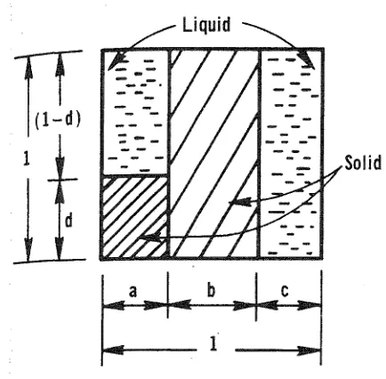
considered. A model was proposed to show the fractional cross-sectional path of the
current through the cement paste as shown in Figure 2.1, where d is the length of the
current path through the conducting solid, c represents the length of the current path
through the solution, b represents the length of the current path through the "solid"
particles and a represents the cross-sectional area of the solution and conductive solids in
series.
Figure 2.1: Schematic for the conduction of electricity through cement paste
(Taylor and Arulanandan, 1974)
The relationship was made between the parameter b and the strength and elasticity of the
cement paste making b the most important parameter in this study.
The cement paste specimens were 12.7 mm by 38.1 mm and they were tested for their
dielectric constant and conductivity over a frequency range of 1MHz to 100MHz. The
water/cement (W/C) ratios used were 0.3, 0.35 and 0.4 where the electrical properties
were tested after about 24 hours of curing. Along with these specimens 50.8 mm x 101.6
mm cement paste cylinders were cast in order to test the compressive strength of the
It was found that for every W/C ratio the solid-solid contacts increased with time, where
they increased rapidly over the first day and then more gradually during the first week.
Also, it should be noted that only a W/C ratio of 0.3 or 0.35 is needed in order for the
complete chemical conversion of cement to occur, and the parameter b became very
sensitive to the W/C ratio of 0.4 meaning that b is very sensitive to an excess of water
present in a cement paste.
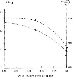
The importance of the parameter b can be seen in Figure 2.2 where it is shown how b can
used to predict the strength of a cement paste at day 7 if it is measured at day 1.
1 ?**• f
? Cay
0.6
0.4
0.2
N. S
\
JL
81199
rm
«wo
0.30 0J2 G.3S G.36 5
WATER - CBIEHT mm BY WEIGHT
Figure 2.2: Strength of cement paste measured and calculated using b parameter
(Taylor and Arulanandan, 1974)
The model using b is conservative when compared to the measured 7 day strength which
is advantageous because it would be safer, as the actual strength would be higher than the
predicted value. Taylor and Arulanandan suggest that it would be possible to create a
field measuring device able to predict the strength of early age concretes from the
has not been studied further beyond the application of the purely academic material of
cement paste and not concrete.
2.2.2 Effect of Water Content in Cement Pastes
Tashiro et al. (1987) investigated the dependence of the electrical resistivity on the
evaporable water content and pore-size distribution of hardened cement pastes. The three
different cements used in this study were ordinary Portland cement (OPC), alumina
cement (AC) and ultra-rapid hardening cement (URHC).
The water/cement ratio used in the cement pastes was 0.4 and the moulds used were 15
mm x 40 mm x 15 mm with two 6 mm x 25 mm steel electrodes spaced at 5 mm. The
specimens were cured at 20°C for one day and then removed from the moulds and dried
in an oven at 60°C to evaporate any water present in the paste. The specimens were
cooled at 20°C and the electrical resistance was measured along with the weight. The
evaporable water content was measured by the difference in this weight and the weight of
the specimens after drying in an oven at 100°C for 12 hours.
Figure 2.3 shows the relationship between the log of the resistivity and the reciprocal of
the water content for each curing time of 3, 7, and 28 days.
- I I
: to
•
T
•ft
1 1 - l — - t ~
J
/
I I I
-• ~
I
4 S » 10 12 14 16 4 « B 10 B 14 4 6 B » K 14
I/w (J"') !/» to"1) //w ($•<!
% ! ' « ' I Variation of electrical rcsklsvily with the reciprocal of the svaporabte water conterJ, tv, far hardened OPC, she curing times are (aj 3 d a p . (h) 7 day;, and fc) 2S days.
Figure 2.3: Variation of resistivity of cement pastes with the reciprocal of water
content
The magnitude of the resistivity remained relatively the same but the slope of the line in
Figure 2.3 (C) increases with time. Figure 2.4 shows the change in the slope C with time
which shows that the slope levelled off by the time the concrete was fully cured at 28
days.
0.6
0.5
0.4
0.3
0.2
O.i
^ °—
- / ^
"(
l - 1 I I i i
10 15 20 25 Curing time (day)
30
Figure 2.4: Variation of slopes from Figure 2.3 with time
(Tashiro et al., 1987)
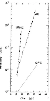
Figure 2.5 shows the variation of the resistivity with which cement type is used. The C
value and resistivity of the AC and URHC cements is considerably higher than that for
OPC.
s e s e H e
J/w tjr'!
Figure 2.5: Variation of resistivity with the reciprocal of water content of different
This result shows that the slope C reflects the difference between the curing time and the
type of cement used. A test of the pore volume was also performed using a mercury
penetration porosimeter, with the results displayed in Figure 2.6.
75 750 Pore radius ( nm !
7500 75 750
Pore radius ( nm )
7S00
Figure 4 Pore-size distributions of various hardened ccmon! pastes; (a) OPC (curing time .1 days), (b) OPC (7 days), (c) OPC (28 days), (d)
AC (7 days), and (e) URHC (7 days).
Figure 2.6: Pore size distribution of different cement pastes
(Tashiro et al., 1987)
From the figure it was concluded that OPC creates a cement paste with more pores of
smaller size than that of AC and URHC while also containing larger pores on average
than AC and URHC. In conclusion of this study, it was found that the C value can
characterize hardened cement pastes with different curing times and types of cements.
This study presents a clear difference in the electrical properties of cement paste, when
there is a change in water content or the type of cement used. The only suggestion for this
study would be that the electrical measurements were taken every day in order to create a
full data set for the proposed C value and how it varies with time.
2.2.3 Impedance of Cement Pastes
McCarter et al. (1988) completed research with the intent of finding the impedance
response of cement paste over a large frequency range at different times during the
hardening process. The frequency range used in this study was 20 to 110 MHz, and the
water to cement ratio of 0.3, the size of the specimens was not given in the report. This is
a vital piece of information that is needed when considering cement paste as a dielectric,
as the impedance is dependent on the size of the specimen. The author should have
provided this information in the article in order for others to compare their work or so
research could be duplicated. Regardless of this, the impedance plots produced show a
familiar shape of a straight line at low frequencies then a semicircular arc after
intercepting with the Real Impedance Axis. The bulk resistance is given by the intercept
and was found to increase with time as the values given were: 190 Q. at 1 day, 404 D, at
14 days, and 528 Q at 25 days. The frequency at which the cement paste relaxes
(Imaginary impedance lowers) decreased with time, indicating that as the cement paste
aged the capillary pores constricted and slowed the current passing through the paste.
The conclusion made was that it could be possible to give a quantitative measure of the
degree of hydration of a cement paste. While a more interesting conclusion to be made is
that the impedance plot formed for cement paste bears the same shape as that of mortar
and concrete found in other studies. This would give further evidence into the fact that in
concrete or mortar the current passes primarily through the cement paste. Even though
the author did not make this conclusion this study was informative and remains important
when attempting to classify the electrical mechanics of cement based materials.
2.2.4 Effect of Water Type on Cement Paste
The objective of the research performed by Wahed and Hekal (1989) was to study the
effect of the water type of a cement paste on its conductivity.
They used three different cement types: Portland cement, slag cement, and blended
cement. The slag cement consisted of 60% Portland cement, 35% blast furnace slag, and
5% gypsum, while the blended cement consisted of 65% Portland cement, 15% blast
furnace slag, 15% cement kiln dust, and 5% gypsum. The different cement types were
mixed with either regular drinking tap water or chloride solution or sea water or sulphate
solution or ground water in order to attain a liquid to cement ratio of 0.3. The specimens
used for the conductivity measurements were cast in cylinders with an internal diameter
cement pastes cylinders, and a conductometer was used to measure the conductivity at
20°C for the first 5 hours after mixing. Conductivity-time curves were established for all
of the different specimens where each curve shared the common characteristic having a
single maximum conductivity achieved during the early stages of hydration.
Figure 2.7 shows the conductogram for Portland cement. The figure illustrates tap water
causes the lowest conductivity and the ground water and MgS04 solution provide similar
conductivity.
Figure 1 Conductograms of Portland
cement paste: (a) tup water, (b) NaC! solu-tion, (c) sea water, (d) MgSO,, solution and (e) ground water.
TIME lh)
Figure 2.7: Conductivity with time using Portland cement paste
(Wahed and Hekal, 1989)
The media containing chloride ions (NaCl and sea water) had a much higher
conductivity, which was likely due to the fact that chloride ions accelerate the effects of
hydrolysis in cement. It was also interesting to note there was a sharp decrease in the
conductivity of the sea water specimen after the maximum, which was likely due to the
sharp decrease of chloride ions as the sea water creates large amounts of ettringite in the
cement paste. The conductogram for the slag cement is shown in Figure 2.8, which shows
!!KJ WJ.5
Figure 2.8: Conductivity with time using slag cement paste
(Wahed and Hekal, 1989)
This likely occurred because the free calcium hydroxide produced during the Portland
cement hydration was consumed by the slag hydration reducing the conductivity. The
specimen cast with the SO4 solution was lower than the tap water and the ground water
specimen was slightly higher. As expected the NaCl solution had the highest conductivity
followed by the ground water due to the phenomenon explained earlier. Figure 2.9
illustrates the conductogram for the blended cement paste, which resulted in markedly
low conductivity values for the tap water specimen as the kiln dust was introduced.
36
Figure i Conductograms irf bicndec
ccnacm paxk: {a) lap water, (b) NaC! ttuu-m>s5. (c) s«s waser, {<!) MgSG* solution ;tnd Ic) ground *;U«.
\
"h-S r!M£ in)
Figure 2.9: Conductivity with time using blended cement paste
The MgSC>4 solution and ground water caused slightly lower conductivities during early
hydration. The sea water specimen had the second highest conductivity initially and it
became the highest after 2 hours when the NaCl specimen lowered significantly. The
NaCl specimen had the highest initial conductivity and two maximums before decreasing
sharply after 2 hours.
Wahed and Hekal (1989) made several conclusions including the fact that different water
types and cement substitutions can change the electrical response of cement pastes. This
has application into the fact that it could be possible for popular cement additives to
change the electrical response of concretes. If this was possible then the presence of these
additives could be studied in a certain concrete mix, or their presence could be accounted
for when taking electrical measurements on a concrete specimen.
2.3 Mortar
2.3.1 Effect of Water Content on the Electrical Impedance of Mortar
Berg et al. (1992) performed one study found on mortar. The objective was to determine
how the dielectric response of cement mortar depends on the water content in a wide
frequency range. The aim was to make use of dielectric measurements as an indicator of
water content in cements, mortars, and concretes although only mortars were studied.
The specimens used were 80 mm x 80 mm cubes of mortar with the water/cement (W/C)
ratios of 0.5, 0.62 and 0.78. Three polished 40 mm x 40 mm nickel plates were embedded
at a distance of 10 mm and 20 mm apart to ensure electrode polarization was easily
distinguishable from bulk conduction effects. The specimens were allowed to harden for
24 hours with most of the specimens sealed in plastic to ensure evaporation occurred
orthogonal to the electrodes. One specimen of each W/C ratio was completely sealed in
plastic. The specimens were stored in air for 3 months with several stages of oven
treatment to see the effects of continuing hydration. The final heat treatment was
performed for 24 hours at 378K (106°C) to remove any weakly bound water referred to
as evaporable water. It was shown that the higher the W/C ratio the higher the percentage
The complex impedance (Z = Zi + Z2J) was found by applying a small sine voltage to a
pair of electrodes and measuring the current moving through the concrete, in the
frequency range of 10"3 to 107 Hz. The first electrical properties tested were the real and
imaginary capacitance, which were tested at 3 days with no heat treatment, 74 days with
no heat treatment, 74 days with a heat treatment for 24h at 333K, 74 days with a heat
treatment for 24h at 363K, and 74 days with a heat treatment for 24h at 378K.
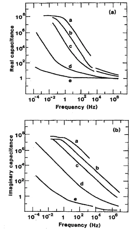
The results for the real capacitance are shown in Figure 2.10 (a), where it can be seen that
the real part of capacitance decreases with frequency, curing time, and increasing heat
treatment. It should be noted that the values of the real part of capacitance seemed to
converge at higher frequencies regardless of curing time or heat treatment. The results for
the imaginary part of capacitance are shown in Figure 2.10 (b), where it can be seen that
the imaginary capacitance also decreased with frequency, curing time, and increasing
10"4 10"2 2 A
10 10*
Frequency (Hz)
1G~4 10"2 1 10" 10^
Frequency (Hz)
10"
FIG. I. (a) Real and (b) imaginary parts of the complex capacitance of cement mortar with water/cement ratio 0.78 are depicted as a function of frequency. The capacitance is given in units of the permittivity of space. The measurements were taken after storage of the sample for (a) 3 days, (b) 74 days in air and after heat treatments for (c) 24 h at 333 K, (d) 24 h at 363 K. and (e) 24 h at 378 K.
Figure 2.10 (a) & (b): Variation of real and imaginary capacitance with frequency
(Berg et al., 1992)
The imaginary impedance maintained more variation at higher frequencies than the real
capacitance and it did not seem to converge. The real and imaginary impedances were
also measured and shown for the specimen with a water/cement ratio of 0.78 in Figure
REAL IMPEDANCE <ktl)
1 9
REAL IMPEDANCE CM ft)
FIG, 2. The imaginary part of the impedance is shown as a function of the real part for mortar with a W/C ratio of 0.78, A constant high frequency capacitance has been subtracted. Points denote experimental values while lines are drawn as a guide for the eye. Frequency values for some experimental points are given in the figures. The measurements were carried out after heat treatment during (a) 24 b at 333 K. and (b) 24 h at 363 K. An equivalent circuit that describes our results is given as an inset in (b). Here Ct and C2 are constant phase elements, while R2 denotes the
bulk dc resistance and a is the phase angle.
Figure 2.11: Complex impedance plot for mortar
(Berg et aL, 1992)
The features of the plot included a straight line at low frequencies and a semi-circular arc
with the centre below the axis at high frequencies. The straight line is indicative of a
constant phase element (CPE) Ci and the semi-circle signifies a resistance (R2) and
another CPE (C2) in parallel, which was in turn the proposed circuit model of mortar. The
dielectric response of the element Ci was proven to be due to electrode polarization, and
therefore the other elements of the circuit described the bulk dielectric response of the
mortar. The element R2 was indicated by the intersection with the real impedance axis in
the complex impedance plot, while the element C2 can be calculated by the equation:
C7 = C 02
(r
(2.1)Where C02 is the amplitude and f0 is the characteristic frequency. The exponent n2 can be
obtained from the angle a by the equation:
The amplitude C02 was obtained numerically from the maximum point of the
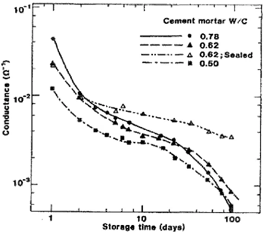
semi-circular arc in the impedance plot. The conductance of the specimens was also measured
over a period of 100 days; the conductance was seen to decrease with time in Figure 2.12,
where initially the conductance was higher with increased water content.
Storage t!m«> (days)
FIG. 3, Conductance as a function of storage time after preparation for cement mortars with different W/C ratios s$ given in the figure. Results for three samples open to air and a sealed sample with W/C ratio 0.62 arc given.
Figure 2.12: Variation of conductance with storage time
(Berg et al., 1992)
While at the end of the storage period the specimen with the highest water content had
the lowest conductance, which is due to the fact that this specimen had a higher rate of
evaporation than the other specimens and it had lost almost all of the evaporable water by
the end of the storage period.
The amplitude of C02 was found to be a function of the water content and was
independent of the W/C ratio for specimens with a water content greater than 0.4. The
exponent n2 was found to be around 0.7 in this experiment, which agreed with the work
value of C2 could be modeled for any cement mortar at any frequency if the amplitude of
the said mortar was known. In conclusion it was noted that the higher the W/C ratio of a
mortar the higher the initial conductance would be, while also the higher the W/C ratio of
a mortar the lower the final conductance would be. Therefore it was proposed that the
dielectric response of mortar could be used to estimate the degree of curing as well as the
original water content of an unknown mix. An equivalent electric circuit was proposed to
be a CPE (C2) in parallel with a resistance, where the values of the necessary parameters
were discovered making the use of this equivalent circuit very plausible to model the
dielectric response of a given mortar if the amplitude is known.
This research was helpful in the sense that it helps develop the theory behind the
conduction of electricity through a cement material like mortar, and has applications to
the masonry industry where it might be possible to estimate the quality or W/C ratio of a
given mortar using electrical methods.
2.4 Concrete
2.4.1 Electrical Resistivity of Concrete
Whittington et al. (1981) tried to find a relationship among the resistivity of concrete, the
ratios of the concrete mix, and the electrical properties of the components of concrete.
Another goal of the research was to determine a relationship between the conduction of
electricity through concrete and a proposed electrical model.
The importance of this research seems to be that it was the first study on the resistivity of
concrete giving the expected result of the electrical resistivity increasing with time. It was
proposed that the electrical current applied to concrete would have three possible paths
through the concrete including: through the aggregate and cement paste in series, through
aggregate particles in direct contact with each other, and through the cement paste only.
A schematic is shown in Figure 2.13 which shows the approximate resistivity of the
concrete if it took the path indicated in the figure, it should be noted that these values
were assumed due to previous research and should not be taken as actual measured
(a) (b) (c)
y x z
Figure 2.13: Conduction model for concrete
(Whittington et al., 1981)
The figure was helpful in quickly showing that the resistivity of concrete will be much
lower if the current only passes through the cement paste and not through the aggregate,
as the resistivity of the aggregate is several orders higher than that of the cement paste.
Such it is that electrical current will take the path of least resistance through the concrete
and will thus pass mostly through cement paste explaining why the resistivity of the
concrete is much closer to that of cement paste than the aggregate (Concrete resistivity =
25 to 45 Qm, Cement Paste resistivity = 10 to 13 fim and Aggregate resistivity = 5xl03
to lxl06fi-m).
After concluding that the current would mostly pass through the cement paste
Whittington et al. considered whether the cement paste could be broken down into two
components being the free evaporable water and the cement-water paste, and whether the
resistivity could be quantified for each component. It was brought to the reader's
attention that the amount of evaporable water present in concrete was almost impossible
to quantify, as it was difficult to determine the electrical resistivity of the evaporable
water and it would also be difficult to determine the electrical resistivity of the
compounds of hydration. And it was concluded that taking the paste as a whole which
would control the overall resistivity of the concrete, was a more than reasonable
assumption. The formation factor (F) was a concept introduced as the ratio of the
resistivity of the composite to the resistivity of the matrix, which in the case of concrete
specimens used were 100 mm cubes with brass plate electrodes on either side of the
concrete which also acted as part of the mould during the first 24 hours of specimen life.
Along with the 100 mm cubes of concrete, 70 mm mortar cubes were tested for the
formation factor because of the high fractional volume of cement paste. There were many
different mixes used in the tests as outlined in the paper using normal Portland cement,
oven-dried fine aggregate with a specific gravity of 2.65 and coarse aggregate with a
grain size no larger than 13 mm and a specific gravity of 2.61. Six specimens were cast
for each concrete mix at each W/C ratio. The specimens were removed from the moulds
after 24 hours and cured in a water bath at 23°C. The weight of the cubes was measured
in order to calculate the density before they were submerged in the water bath. The
electrodes were attached to the specimens using a low-resistance cement paste, so the
measured resistance values would not be changed. There were also some specimens
stored outdoors beneath 200 mm of sand after 13 days of curing inside; this was tested in
order to simulate concrete with an outdoor lifespan. Due to the polarization effects
discussed earlier, the resistance was measured directly from the specimens using a
non-disclosed ohmmeter using a low-frequency alternating current. All of the specimens were
tested over a 3 to 4 month period, while the concrete stored outdoors was considered to
have experienced a reasonable amount of climate change to simulate the life of an
outdoor concrete.
The results for the early life of the concrete and cement paste was found to show a
gradual increase of resistivity in concrete until the concrete sets and then the resistivity
increases more rapidly, while the cement paste had decreasing resistivity in the first 5
hours before increasing. This decrease in resistivity was thought to be the cause of the
hardening of the cement paste being an exothermic reaction which would increase the
temperature and therefore, lower the resistivity or due to an increase in the number of
ions going into solution. The decrease in resistivity was not present in concrete likely
because the concrete has a lower amount of fractional volume of cement paste, or
possibly due to the coarse aggregate accepting the heat transfer from the chemical
reaction and negating a decrease in resistivity. It was important to note the relationship
between the water/ cement ratio and resistivity was inversely proportional, with an
the water bath were found to reach an almost constant resistivity by about 20 days
regardless of the W/C ratio, where the increase in resistivity during the first 20 days was
likely due to the loss of evaporable water. The concrete specimens that were cured
outdoors were found to have a more variable resistivity over time than the other
specimens, and the change in resistivity was assumed to be due to the temperature change
over time, which was outlined earlier in the paper to vary with temperature. It was also
interesting to note that the temperature coefficient (a) of the cement paste was found to
be 0.022/°C and the temperature coefficient of most electrolytes is 0.025/°C. The last
thing tested in this study was the formation factor (F) which was found to follow the
equation F=1.04(p"1'20 where (p represents the fractional volume of cement paste present in
the concrete tested. This negative linear relationship shows that as (p increases the F
decreases which validates the theory shown earlier in the paper, F for a certain mix and
W/C ratio is reasonably constant and that the resistivity could be found for mixes with
different fractional volumes than the ones used in the study.
The final conclusions of this study were that as the W/C ratio of concrete increased the
resistivity decreased showing that the strength decreased as the resistivity decreased.
Since the resistivity of the aggregate is almost infinite when compared to that of the
cement paste, showing that the resistivity of the concrete is almost completely dependent
on the resistivity of the cement paste in the concrete. The electrical resistivity of concrete
was directly related to the rate of hydration of the cement paste, suggesting that the
strength of the concrete could be linked to the resistivity. This study was very important
in setting up the framework for concrete to be studied in an electrical sense by using
many different mixes and W/C ratios making the link between many of these variables in
concrete and how they affect the resistivity of concrete. The realization that current
travels almost entirely through the cement paste in concrete is an important discovery,
because it creates a solid foundation for understanding how concrete acts as an electrical
material. The use of specimens that were stored outdoors was an interesting idea but the
data does not seem as relevant because it was not used in the calculation of the formation
2.4.2 Dielectric Properties of Concrete
The intent of a study by Wilson et al. (1984) was to find if high-frequency impedance
measurements could detect entrapped air inside of cast concrete. The other objective was
to find the effect of increasing the amount of coarse aggregate on the high-frequency
impedance measurements.
The specimens used were 150 mm cube with electrodes on opposite faces with a coaxial
connection to the impedance analyzer. The basic concrete mix used had water/cement
ratio of 0.5 and cement:sand:coarse aggregate ratio of 1:1.5:3. The variations on this mix
were one specimen with 5% more coarse aggregate, one specimen with 5% more air
volume, and one specimen with 10% more air volume. All impedance measurements
were carried out on the concrete specimens after 6.02 days of setting over the frequency
ranges of 1 to 100 MHz and 500 to 700 MHz.
The results of the lower frequency band were collected in Figure 2.14, which shows that
the impedance steadily declined with frequency up until 30 MHz where it began to
fluctuate.
Figure 2.14: Low frequency impedance plot of concrete
(Wilson et al., 1984)
The fluctuation was accounted to the coaxial to parallel plate transition where minor
resonances occurred. It can be noted that between 1MHz and 10MHz all of the mixes had
a higher impedance as compared to the normal mix, with the high air mix having the
highest impedance and the low air mix having the lowest impedance. At a frequency of
1 MHz the normal mix showed an impedance of around 250 £1 while the other mixes
were all near the 300 Q. mark. The results for the higher frequency range are shown in
Figure 2.15 which shows an increase in aggregate caused a decrease in resonant
frequency, while a large increase in air caused an increase in resonant frequency.
IOOOI
HIGH AIR
500 600 700
FREQUENCY (MHz)
Figure 2.15: High frequency impedance plot of concrete
(Wilson et al., 1984)
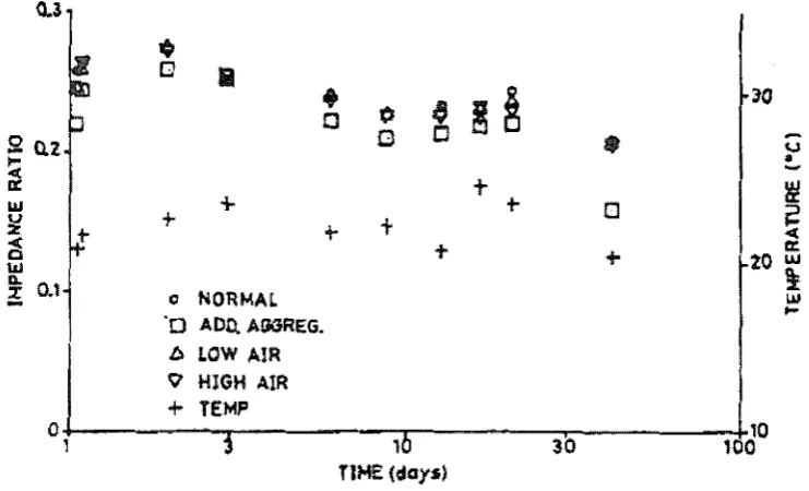
The impedance was also measured at specific days over one month where the specimens
were stored in a water bath until measurements were taken. Over the low frequency range
the impedance at 30 MHz divided by the impedance at 1 MHz appeared helpful as it
showed variation between the specimens. As can be seen in Figure 2.16 the specimens
with added air had an impedance ratio closer to that of the normal specimen than the
0.3
m
j
« U24
5
a. <->
at
o vu X 0.1
H^
D
e
o NORMAL O ADQ.ASSREQ.
& LOW AIR
<? HIGH AIR + TEMP
g s&
T
^ — TIME Ways)a
+•
30
h30
< er 20 J"
Si
.10 100
Figure 2.16: Variation of impedance and temperature with time
(Wilson et al., 1984)
This study indicates that it is possible to detect the difference between a specimen with
additional air voids and a specimen with excess aggregate. Excess air voids could
possibly result in lower strength.
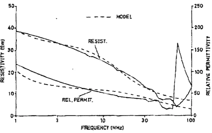
The resistivity and relative permittivity were also calculated using the impedance data
collected at 6.02 days. The results for the lower frequency range are given in Figure 2.17
showing a steady decrease in both resistivity and relative permittivity as frequency
increased, while the resistivity and relative permittivity had values of 40 CI and 125 CI
50-, rZ5Q
FHtqUEKCV (MHz)
Figure 2.17: Low frequency plot of resistivity and relative permittivity
(Wilson et al., 1984)
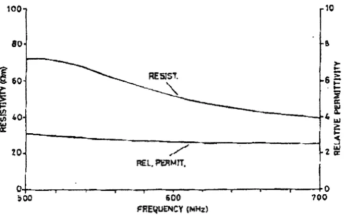
The higher frequency range had the results in Figure 2.18 yielding a resistivity over 70 Q
and relative permittivity of 3 at 500 MHz. It should be noted that the results at both
frequency ranges should be questioned again due to the coaxial line transition, which
were found at about 70 MHz. The very high values of the relative permittivity at low
frequencies were estimated to be due to Maxwell-Wagner effects, which assume the
current passes through the water which would have a relatively high conductivity. A
proposed model for this effect is also shown in Figure 2.17 which accounts for randomly
oriented conducting needles and a continuous water channel with a very thin insulating
1001 r1 s
304 * U
—' — — — - - " " — — — — JJ
20- ^ -tec R£L, PERMIT.
0 4 ' i • "i '•••• i — - i - » - i • 1 ' *"" " l r0
*»QQ 600 700 FREQUENCY (WHz)
Figure 2.18: High frequency plot of resistivity and relative permittivity
(Wilson et al., 1984)
The model gives the general shape of resistivity and relative permittivity but there are
discrepancies between the model and measured values. The variation in the values was
likely due to the fact that the model assumes the conducting needles throughout the
cement paste matrix are the same length, even though concrete can have a great variation
in pore sizes.
In conclusion it was found in this study that it was possible to detect small variations in
the constituents of concrete. The researchers could have described the impedance
measurements at different days and if there was as much variation between mixes as there
was at 6.02 days. If the variation was noticeable at 1 day or earlier, there could be more
application for this research in terms of detecting the quality of a certain concrete after it
is cast in place. Also, it would have been beneficial to see the variation between the
mixes beyond 6.02 days and whether the variation increases with time. It is possible the
impedance measurements could have been used on concrete that is already in service and
whether it has experienced deterioration by comparing it to a test specimen of the same
2.4.3 Relationship between Resistivity and Strength of Concrete
The work of Whittington and Wilson (1986) had the intention of creating a
non-destructive test method for concrete using the measurement of electrical properties, with
the final result being a quality control test for structural concrete. The purpose of the
study was to make an alternative test of concrete strength in comparison to the current
tests used to measure the mechanical properties of concrete, as the electrical properties
are comparable to the mechanical properties because they both depend on the same
chemical reactions that take place in concrete during the hydration process.
An in-depth analysis of the chemistry involved in the hydration on cement was performed
in order to appreciate the significance of the electrical parameters used. The main purpose
of this analysis was to explain that the water and cement reacted to produce a matrix of
compounds making the cement paste, which locks the fine and coarse aggregate together
to create concrete. The mechanical and electrical properties of concrete depend on the
amount of hydration that the components of concrete have achieved, the way the water is
distributed and the condition of the concrete matrix. When it comes to the electrical
properties of concrete it can be considered to be a large amount of insulating material
(coarse aggregate) imbedded into a conducting matrix of cement paste. The concrete was
modeled as two resistances in parallel, one of them representing the aggregate and the
other representing the cement paste. Even though the cement paste had a lower volume
ratio than the aggregate, it had a lower resistivity and is therefore expected to control the
resistivity of the concrete overall.
The specimens used were 150 mm cubes of concrete were used in the experiment along
with two 14 SWG stainless-steel electrodes placed on opposite faces to obtain the
electrical data. One electrode was also fitted with a temperature sensor in order to take
temperature measurements as well. The moulds were made from PVC to accommodate
both the 150 mm concrete cube and the electrodes, and when the mould was removed a
good bond was found between the concrete and the stainless-steel electrodes. The only
concrete mix used in this study incorporated a cement: sand: aggregate ratio of 1:1.5:3
and a water/cement ratio of 0.5. As in previous studies using BS 1881 (1983) as a
until resistivity measurements were made and the specimens were removed from the bath
and allowed to dry for 5 minutes before making the measurements then placed directly
back into the bath. The resistivity data was collected using an automatic measurement
system making it possible to record the data of 15 different specimens at once, for a
complete time cycle of 100 days being the maximum. The specimens were removed from
the water bath using an automatic hoist before each resistivity measurement was taken, at
a frequency of 2.0 kHz using a square wave AC signal. In order to take the temperature
measurements the signal was amplified to 7.2 kHz. The percentage of error in the
resistivity measurements was found to be less than 2% if the resistivity measured was
greater than 1 Q.m, which included most of the measurements taken in the study.
The results of the experiment are greatly concluded in both Figures 2.19 and 2.20. Figure
2.19 shows the change in resistivity over time while Figure 2.20 shows the correlation
between the strength of concrete and the resistivity. The results in Figure 2.19 are as
expected with the resistivity increasing gradually with time until it sets and then
increasing more rapidly when it sets.
* + + + +
J ' • t m i l I I i i m i l |—1 L l l l U I I L J
0.01 0.1 1 10 time, days
Figure 2.19: Variation of resistivity with time
(Whittington and Wilson, 1986)
The conclusion made by Whittington and Wilson was that the curve in Figure 2.19 could
be used in the quality control of concrete, as any concrete with a resistivity measured
outside of this calibration curve would be considered suspect.
60
;AO
* 2 0
5 0
-40
£ 30
; 2o
-"
1
s
1 ,
r- -n l - J
33
[ X J
a
10 20 30 40
corrected resistivity. Om
€0
Figure 2.20: Correlation of resistivity and strength
(Whittington and Wilson, 1986)
Figure 2.20 is very ambiguous as the day at which the strength and resistivity were
measured is not indicated, and was only said to be between 2 to 28 days. The figure also
contains dashed boxes around the data points which indicate the amount of error to be
expected from the values obtained. However, conclusion was made by the author that the
correlation between resistivity and strength is linear and the resistivity of concrete
increases as the strength increases. It should, however, be noted that the increase in
resistivity is very small.
2.4.4 Variation of Electrical Properties of Concrete with Frequency
Whittington and Wilson (1990) attempted to propose certain mechanisms which control
the conductivity and dielectric constant of concrete in order to develop an electrical
model. This electrical model would then be compared with the electrical measurements,
with the validity of the model being discussed.
The concrete specimens were cast in a PVC mould with two stainless-steel electrodes on
opposite faces. The mould was a 150 mm cube with a coaxial line attached to the
electrodes to create a direct link to an impedance analyzer. The specimens remained in
the moulds during all measurements. The measurements were carried out on four
identical specimens at a frequency range of 1 to 100 MHz, using a HP4191A RF
and a cement: sand aggregate ratio of 1:1.5:3. The impedance measurements were taken at
a time of 1 hour after the concrete was mixed and 1 day after the concrete was mixed.
The conductivity at 1 hour was found to be constant at 0.2 S/m until about 20 MHz and
dropped virtually to zero at 100 MHz. While the conductivity at 1 day was found to be
about 0.03 S/m and stayed constant until about 10 MHz and increased to 0.2 S/m at 50
MHz and then back down to zero. The dielectric constant was found to be positive but
declining until 2 MHz when it dropped below zero and remained negative up to 100
MHz. While the dielectric constant remained positive but declining until 50 MHz. The
results of the electrical experiments could be best explained by electrode polarization, the
change in behaviour from homogeneous conduction best described as the
Maxwell-Wagner effect and viscous conduction effects.
Electrode polarization occurs when ions reach the electrodes and gas is produced, since
concrete is so viscous the gas cannot escape creating another capacitance in parallel to the
resistive bulk and causing a low conductivity in concrete. This polarization model is
represented by a capacitor in series with a capacitor and resistor in parallel having the
impedance:
jcoCi l+jo)C2R
Although the circuit can be made into an equivalent circuit of a resistance in parallel with
a capacitor having the admittance:
r = f+;a)C
p(2.4)
While the conductivity (a) and dielectric constant (e) can be postulated by the equations
derived in the text, and were best used to model the conductivity after 1 hour. The result
of this model is seen in Figure 2.21 and shows that the polarization model is not accurate
10 frequency, MHz
Figure 2.21: Comparison of dielectric constant at one hour
(Whittington and Wilson, 1990)
The model is close from 1 to 10 MHz and it was possible that the polarization mechanism
is more complex than the model or the polarization was not complete across the
electrode. The Maxwell-Wagner effect occurs when the frequency of a field is greater
than the critical frequency and the charge carriers cannot redistribute fully. The cause of
the effect is a reduced dielectric constant, an increase in electrical loss and an increase in
conductivity. The model produced by the Maxwell-Wagner equations best fits the
conductivity and dielectric constant after 1 day which can be seen in Figure 2.22 and
Figure 2.23, respectively.
10
frequency, MHz
100
Figure 2.22: Comparison of conductivity at one day
-rnoael
measured
\
frequency, MHz
Figure 2.23: Comparison of dielectric constant at one day
(Whittington and Wilson, 1990)
The Maxwell-Wagner model was close to the measured conductivity in Figure 2.22 at
low frequencies, but the variance increased as the frequency increased. The model in
Figure 2.23 followed the dielectric constant at low and high frequencies. The discrepancy
in the Maxwell-Wagner model was most likely due to the assumption of the volume and
geometry being fixed, when in reality there can be statistical distribution in these
variables. The viscous conduction effect occurs when the ability of an ion to respond to
an alternating electric field is restricted because the frequency has reached a cut-off point.
This electrical model best represented the conductivity after 1 hour as seen in Figure
2.24. The model closely followed the measured conductivity with variance occurring
above 20 MHz.
& 0.2
>
D
C
0.1
r-easured
mode
X—J i i i i i . i
10
frequency, MHz
100
Figure 2.24: Comparison of conductivity at one hour