Evaluating Displacements on a Circular Cylindrical Shell with the Use of
Polynomial Quadrature Method
Eurice de Souza1) and Lineu J. Pedroso1)
1) Grupo de Dinâmica e Fluido-Estrutura, Departamento de Engenharia Civil e Ambiental – Universidade de Brasília, DF – Brazil
ABSTRACT
A polynomial differential quadrature method (PDQ) is proposed for the solution of complex sets of differential equations. In the PDQ method displacements are discretized as matrices whose indexes correspond to spatial coordinates; differential operators are replaced by special matrices embedding contour conditions. So partial differential equations lead naturally to a linear algebraic system easily solvable using the computational apparatus. In order to display the performance of the method, an important problem in the analysis of reactor technology is considered – the evaluation of the displacements on a circular cylindrical shell.
INTRODUCTION
Polynomial methods have been widely used to provide numerical and semi-analytical solutions for complex problems in engineering and mathematical physics [1] for most problems can be described by smooth functions amenable to polynomial approximation.
In [2], the polynomial differential quadrature (PDQ) method was first proposed by Bellman et. al. as an efficient technique for the solution of nonlinear partial differential equations. In [3], a novel technique for the construction of the polynomial differential quadrature matrix for systems described by fourth order differentials is proposed in order to include exact edge conditions. In [4]–[7], the PDQ method has been used for the solution of many structural problems, including plane plates and beams of complex geometries. In [7], the technique proposed by [3] was enhanced and extended for the solution of problems displaying parameter variation or even discontinuities along the domain.
In this paper, it is shown how the method can be implemented to solve a problem governed by high order complex partial differential equations. In order to display the efficiency and versatility of the technique a semi-analytical solution for an important problem of nuclear power plant (a circular cylindrical shell with arbitrary efforts in the radial, azimuthal and vertical directions) is obtained. SYNTHESIS OF POLYNOMIAL DIFFERENTIAL QUADRATURE OPERATOR THEORY
In this section, a brief review of the differential quadrature is given. First, quadrature operators are constructed for a smooth function sampled at the abscissas ( )xi in=0.
Quadrature Operator for a Sampled Smooth Function
For the ease of presentation, consider the elementary polynomials of the set {p xk( )=xk}nk=0. Let P x( ) be a row-vector whose entries are elements of a basis for the polynomials of degreen:
( ) [ 0( ) 1( ) n( )]
P x = p x p x … p x (1)
Let u x( ) be a sufficiently smooth function and let uˆ be a vector of the samples of u x( ) discretized on assigned abscissas ( )xi in=0.
First u x( ) is approximated in terms of the weighted components of P x( ),
( ) ( )
u x ≈P x α (2)
Denoting by P, the discretized version of P x( ) on the assigned coordinates, sample vector uˆ and coefficient vector α satisfy the following one-to-one relation:
1
ˆ ˆ
u ≈ P⋅α ⇔ α=P− ⋅u
(3) Next, differentiation of order k on the function u x( ) can be approximated in the form:
( ) ( ) ( ) 1 0 diag 1, 2,( , )
0 0
ˆ;
k
k k k
d
n n
dx
n Dn
u x ≈P x D⋅ ⋅ =α P x D P⋅ ⋅ − ⋅u = ⎡ ⎤
⎢ ⎥
⎣ ⎦
…
(4)
where Dn is the constant matrix that performs exact differentiation on the vector P x( ); diag .( )
stands for the diagonal matrix with elements “(.)” and the zeros represent zeros or blocks of zeros of appropriate dimensions.
Denoting byuˆ( )k the approximated differentials onthe assigned abscissas, from (4), there results:
( ) 1
ˆ k ˆ,
P
k k k
P n
u ≈Q ⋅u Q =P D⋅ ⋅P−
(5) k
P
Q is the kth order differential quadrature matrix operator associated to the given polynomial basis.
Quadrature Operator Embedding Edge Conditions
Now a scheme is devised to derive a quadrature operator fixing the edge conditions for the smooth function u x( ). Suppose one intends to fix a clamped support on the left and a simple support on the right. For this purpose, consider the set ( ) 2
0
{ k}n
k k
p x =x =+ and let P x( ) be a
row-vector whose entries are elements of a basis for the polynomials of degreen+2: ( ) [ 0( ) 1( ) n 2( )]
P x = p x p x … p + x (6)
In order to impose the specified edge conditions, u x( ) and some of its derivatives are written: ( ) ( ) , ( ) ( ) , ( ) ( )
u x ≈P x ⋅α u x′ ≈P x′ ⋅α u x′′ ≈ P′′ x ⋅α (7)
Let P be the discretized version of P x( ) and P0 and P0′ be the discretized versions of P x( ) and P x′( ) on the left coordinate; also, let Pn and Pn′′ be the discretized version of P x( ) and
( )
P′′ x on the right coordinate. So, sample vector uˆ∗ and coefficient vector α satisfy the relation: 1
ˆ ; ˆ
u∗ =P∗⋅α ⇔ α=P∗− ⋅u∗
(8) where
[ ]
0 0 1 2 1 0 0
ˆ ˆT T; ˆT ; T T T T T T
n n n n n
u∗ u u u u u u u u u P∗ P P P P P
−
⎡ ′ ′′⎤ = ⎡ ′ ′′ ⎤
⎣ ⎦ … ⎣ ⎦
Using (8), differentials on the sampled coordinates are approximated as uˆ( )k =PDnk+2⋅α, or
( ) ( )
( ) 1
2 0 0
ˆk k ˆ ; k k k
n P n n
P P
u Q∗ u∗ Q∗ PD P∗− q q Q q q
+ ⎡ ′ ′′⎤
= ⋅ = ⎢⎣ ⎥⎦ (9)
Using the columnwise partition suggested in (9), there results the quadrature formula: ( )
0 0 0 0
ˆk k ˆ
P n n n n
u ≈Q u+q u +q u′ ′ +q u +q u′′ ′′ (10)
with obvious simplification in the case of trivial edge conditions.
EXAMPLE: EVALUATING DISPLACEMENTS ON A CIRCULAR CYLINDRICAL SHELL
In order to illustrate the application of the method proposed for the solution of partial differential systems of equations an important component of nuclear power plants – a cylindrical shell structure – is considered.
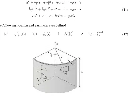
In Fig. 1, the cylindrical shell and orthogonal displacements u, v and w are sketched. The differential equations for the cylinder displacements are governed by the Donnell equations:
1 1
2 2
1 1
2 2
4
u
. x
r
u u v w p r
v v w p r
u v w k w p r
ν ν
ν ν
φ
ν
ν
λ
λ
λ +
−
+ −
∇
′′+ + ′ + ′ = − ⋅
′ + ′′+ + = − ⋅
′ + + + =
ii i
i ii i
i
(11)
where the following notation and parameters are defined
( )
( )
( )
2
2 1
1 1
12 /
(.) (.) (.) (.) h h
r E r
x r φ k λ ν
−
∂ ∂ −
∂ ∂
′ = i = = = ⋅
(12)
Fig. 1. Cylindrical Shell Structure and Assigned Coordinates
and ∇4(.) is the biharmonic operator that is obtained by the application of the Laplacian twice:
(
)
4(.) 2 2(.) (.)′′′′ 2(.)′′ (.)
∇ = ∇ ∇ = + i i + i i i i
(13)
The boundary conditions are given below
( ) at the curved edges: 0, 0, 0, 0
( ) at the straight edges: 0, 0, 0, 0
a u v w w
b u v w w
′ ′′
⎧ = = = =
⎪⎪
⎨⎪ = = = =
⎪⎩ i (14)
Performing Quadrature with respect to x – “( ). ” Sampling
For w the sampling is carried out aiming at the edge conditions on the bottom and on the top. As to sampling on u and v, these are assigned to be compatible to sampling on w displacements.
0 0 0 0
ˆ ˆT T; ˆ ˆT T; ˆ ˆT T
n n n n
w∗ = ⎢⎣⎡w′′ w w w w′′⎤⎦⎥ u∗ = ⎡⎣⎢u′ u u′⎤⎦⎥ v∗ = ⎣⎡⎢v v v ⎥⎤⎦ (15)
where uˆ, vˆ and wˆ represent the internal samples depending on φ and “∗” denotes sampling to include boundary conditions.
2 2 2
1 1 1 1 1 1
ˆ ˆ ˆ ˆn T; ˆ ˆ ˆ ˆn T; ˆ ˆ ˆ ˆn T;
w = ⎢⎣⎡w w … w − ⎤⎦⎥ u = ⎣⎡⎢u u … u − ⎦⎥⎤ v = ⎣⎢⎡v v … v − ⎥⎦⎤ (16)
Quadrature matrices can be built for u, v and w internal coordinates with respect to x using (10):
[
, ,]
;[
, ,]
;[
, ,]
i i i i i i i i i i i i
u u T u u B v v T v v B w w T w w B
Q = Q Q Q Q = Q Q Q Q = Q Q Q (17)
where the superscript “i” denotes ith differential polynomial quadrature matrices with respect to x; Subscripts ‘T’ refer to top-edge and ‘B’ refer to bottom-edge coordinates. Using (17) in (15), yields:
[
]
[
]
[
]
[
]
[
]
[
]
[
]
[
]
1
2 2 2 1 1 1 1 1 1 1
, , 2 2 , , , ,
1 1 1 1 1 2 2 2
, , , ,
2 2
1 1 1 4 4 4 2 2 2
, , , , , , ˆ ˆ ˆ ˆ ˆ . ˆ ˆ ˆ ˆ ˆ . ˆ ˆ ˆ ˆ ˆ ˆ 2
u T u u B v T v v B w T w w B x
u T u u B v T v v B
u T u u B w T w w B w T w w B
Q Q Q u u Q Q Q v Q Q Q w p r
Q Q Q u Q Q Q v v w p r
Q Q Q u v w k Q Q Q w Q Q Q w w
ν ν ν ν φ ν ν λ λ + ∗ − ∗ ∗ + ∗ − ∗ ∗ ∗ ∗ + + + = − + + + = − + + + + + ii i
i ii i
i
(
ii iii)
ˆ .r
p rλ
= i
(18)
Eliminating the trivial edge conditions in (18), there results:
1
2 1 1 1
2 2
1 1 1 2
2 2
1 4 2
ˆ ˆ ˆ ˆ ˆ ˆ ˆ ˆ ˆ ˆ u ˆ ˆ ˆ ˆ ˆ
ˆ 2 ˆ
u v w x
u v
u w w r
Q u u Q v Q w p r
Q Q v v w p r
Q u v w kQ w kQ w kw p r
ν ν ν ν φ ν ν λ λ λ + − + − + + + = − ⋅ + + + = − ⋅ + + + + + = ⋅ ii i
i ii i
i ii iiii
(19)
Performing Quadrature with respect to φ – “( ). ” Sampling
Each uˆ, vˆ and wˆ vector coordinate depends on φ variable. So, for uˆk( )φ , vˆk( )φ and wˆk( )φ coordinate sampling is performed with respect to φ aiming at the edge conditions on the straight edges for wˆ ,k uˆk and vˆk:
,0 ,0 , , ,0 , ,0 ,
ˆk k k ˆk k m k m ; ˆk k ˆk k m ; ˆk k ˆk k m
w∗ = ⎡w• w w w w• ⎤ u∗ = ⎡u u u ⎤ v∗ = ⎡v v v ⎤
⎢ ⎥ ⎢ ⎥ ⎢ ⎥
⎣ ⎦ ⎣ ⎦ ⎣ ⎦ (20)
The internal coordinates are given by:
,1 ,2 , 1 ,1 ,2 , 1 ,1 ,2 , 1
ˆk k k k m ; ˆk k k k m ; ˆk k k k m
w = ⎡⎢⎣w w … w − ⎤⎥⎦ u = ⎣⎡⎢u u … u − ⎥⎦⎤ v = ⎡⎢⎣v v … v − ⎤⎦⎥ (21)
Denoting, respectively, by RuT, RTv and RTw the quadrature matrices to approximate differentiation on u, v and w displacements with respect to φ, the previous procedure can be used to obtain:
1
2 1 2 1 1 1
2 2
1 1 1 1 2 2 1
2 2
1 1 4 2 2 2 4
T T
u u v v w x
T T T
u u v v w
T T T
u v w w w w r
Q U UR Q VR Q W P r
Q UR Q V VR WR P r
Q U VR W kQ W kQ WR kWR P r
ν ν ν ν φ ν ν λ λ λ + − + − + + + = − ⋅ + + + = − ⋅ + + + + + = ⋅ (22)
where U,V and W are, respectively, the matrices associated to internal displacements u, v and w:
1 2 1 ˆ1 ˆ2 ˆ 1 ˆ1 ˆ2 ˆ 1
ˆT ˆT ˆT T ; T T T T ; T T T T
m m m
U = ⎡⎢⎣u u … u − ⎤⎥⎦ V = ⎣⎡⎢v v … v − ⎥⎦⎤ W = ⎡⎢⎣w w … w − ⎤⎦⎥ (23)
Let u, v and w be the vectors formed, respectively, by the stacking of the columns of displacement matrices U, V and W and let px, pφ and pr be the vectors formed, respectively, by the stacking of the columns of the effort matrices Px, Pφ and Pr. Using Kronecker product properties the system can be written in the linear standard form:
( ) ( ) ( )
( ) ( )
( ) { ( ) }
1
2 1 2 1 1 1
2 2
1 1 1 2 1 2 1
2 2
1 1 4 2 2 2 4
u u x v v w x
u u v x v w x
r
u v x x w w w w x
I Q R I R Q I Q u p r
R Q R I I Q R I v p r
w p r
I Q R I I I k I Q R Q R I
ν ν
φ φ
ν ν
φ φ
φ φ φ
ν
ν
λ λ λ
+ −
+ −
⎡ ⊗ + ⊗ ⊗ ⊗ ⎤⎡ ⎤ ⎡− ⋅ ⎤
⎢ ⎥⎢ ⎥ ⎢ ⎥
⎢ ⎥⎢ ⎥ ⎢ ⎥
⎢ ⊗ ⊗ + ⊗ ⊗ ⎥⎢ ⎥= −⎢ ⋅ ⎥
⎢ ⎥⎢ ⎥ ⎢ ⎥
⎢ ⎥⎢ ⎥ ⎢ ⋅ ⎥
⎢ ⊗ ⊗ ⊗ + ⊗ + ⊗ + ⊗ ⎥⎢ ⎥⎣ ⎦ ⎢⎣ ⎥⎦
⎢ ⎥
⎣ ⎦
(24) RESULTS
Formula (24) was implemented in a personal computer using the software MATLAB®.
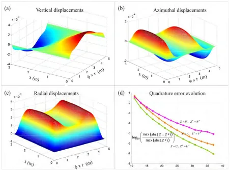
A 3m high and 2cm thick steel cylindrical shell submitted to a pressure of 1MPa was considered. Also the shell radius is 3m and its angle is 1.6 radians and the Young modulus of the material is 200GPa and its Poisson ratio is 0.28. For the displacements u,v and w internal coordinates x and φ where discretized in n m, =11,13, , 39… discrete levels. Interpolation was used to generate the smooth graphs. In Figure 2 (a)–(c) the displacements are displayed with respect to the rectangular projection abscissas x and φ×r.
Fig. 2. Cylindrical shell displacements ,U V and W are displayed in (a), (b) and (c). In (d) the evolution of convergence of approximation is portrayed.
In Figure 2 (d), the logarithmic criterion log10(max(abs(Z Z- ∗))/ max(abs(Z∗))) is used
to compare the values of the approximate displacements Z =U V, and W with the displacements obtained for Z∗=U V∗, ∗and W∗, where the symbol “*” denotes the approximation obtained for
39
n= =m . All the matrices used in the comparisons refer to the interpolated smooth data. CONCLUSIONS
A polynomial differential quadrature method (PDQ) was used for the solution of complex sets of differential equations arising from the problem of evaluation of the displacements on a circular cylindrical shell – a common component used in the construction of nuclear power plants.
The method is very easy to implement. The polynomial bases for each displacement function are chosen aiming at the particular edge conditions. So, once the quadrature matrices are built, it is straightforward to transform the partial differential system into an algebraic linear system. For instance, if the x coordinate is selected as the vertical coordinate and φ is chosen as the horizontal coordinate, differentials with respect to x are simply replaced by quadrature matrices of appropriate orders on the left; differentials with respect to φ are simply replaced by quadrature matrices of appropriate orders on the right.
The results obtained for the problem proposed are quite satisfactory even for mild polynomial approximations. However, quadratures of orders so high as 39 have been tested yielding a stable, well-conditioned and fast-solvable standard system Ax =b.
A critical point in the construction of the quadrature matrices is the inversion of special Vandermonde matrices. In the present implementation, only the selection of non-uniform Chebyshev abscissas was performed with excellent results. In practice, using Chebyshev polynomial bases, it can be expected that quadratures of much higher order could be used to solve problems demanding such sophistication.
ACKNOWLEDGEMENTS
The authors are grateful to ELETRONORTE for the financial resources (equipment) and for the grants (scholarships) left at the disposal of the authors for the achievement of this research.
REFERENCES
1.http://www.LORENE.obspm.fr/school/polynom.pdf; Maintained by the Laboratoire de L’Univers et de ses Théories (LUTH), CNRS, Observatoire de Paris, as seen in 4/12/2005.
2.Bellman, R, Kashef B.G.and Casti J. Differential quadrature: a technique for the rapid solution of nonlinear partial differential equation, J. Comput. Phys. 10 (1972), pp. 40 – 52. 2005.
3.W. Chen, A.G. Striz and C.W. Bert. A new approach to the differential quadrature method for fourth-order equations, Int. Journal for Num. Meth. Vol. 40, pp. 1941 – 1956, (1997).
4.deSouza, E. Technical Report of Research RTP-ES09 - 12/2005. Solution for the Beam Equation Using the Differential Quadrature Method (in Portuguese). (2005).
5.deSouza, E. Technical Report of Research RTP-ES11 - 01/2005. Solution for Plate the Equation Using the Differential Quadrature Method (in Portuguese). (2005).
6.deSouza, E. and Pedroso, L. J., Solution for the Laplace equation based on the polynomial differential quadrature method for the evaluation of the temperatures in the interior of a typical dam, Proceedings of the XXVII CILAMCE – Iberian Latin American Congress on Computational Methods in Engineering, Sept 3-6, 2006 – Belém, Pará – Brazil.
7.deSouza, E. and Pedroso, L. J., Solution for the Beam Equation involving Discontinuous Loads or Moments of Inertia through the Polynomial Differential Quadrature Method, accepted for publication in the XXVIII CILAMCE to be held in Porto, Portugal, in June 13–15 (2007).