Estimation of the Parameters in a Class of Dynamic Network Models.

(1)

ABSTRACT

ZHAO, WEI. Estimation of the Parameters in a Class of Dynamic Network Models. (Under the direction of Soumendra Lahiri).

(2)

(3)

Estimation of the Parameters in a Class of Dynamic Network Models

by Wei Zhao

A dissertation submitted to the Graduate Faculty of North Carolina State University

in partial fulfillment of the requirements for the Degree of

Doctor of Philosophy

Statistics

Raleigh, North Carolina 2019

APPROVED BY:

(4)

DEDICATION

This work is in honor of

Yu Yi (Mama), and Yinbao Zhao (Papa) Juzi (kitty)

This work is also in memory of

(5)

BIOGRAPHY

The author was born and raised in an industrial town called Dexing Copper Mine, Jiangxi, China in January 1992. She graduated from The Attached Middle School of Jiangxi Normal University in June 2009, and was admitted to Beijing Normal University to study Information Management afterwards. However, after one year of learning, she found her great interest in quantitative fields and changed her major to Statistics without any hesitation. Ranking No.1 among over 30 students, she got her Bachelor’s degree in Statistics in 2014, and was offered a full Teaching Assistantship in North Carolina State University to pursue her PhD in Statistics. During the time in R aleigh, she joined the Sunny Dance Club and performed in Triangle Chinese New Year Festivals in 2016, 2017 and 2018.

(6)

ACKNOWLEDGEMENTS

I would like to thank my advisor, Dr. Soumendra Lahiri for his guidance and help. His gift and proficiency in statistics and researches taught me a lot, and guided me all through my work of this thesis. Moreover, Dr. Lahiri, thank you so much for giving us such good lectures in the courses Advanced Probability and Advanced Time Series that I found my interest and finished my first project of dynamic network. In addition, I feel so lucky to have Dr. Lahiri as my advisor who is so generous to support me with Research Assistantship during my unfunded time. At last, I want to say to Dr. Lahiri, without your support, I wouldn’t overcome the hard time when I was still looking for a job. Your encouragement and understanding gave me much more confidence in myself.

Here I also want to express my sincere thankfulness to all my committee members, Dr. Rui Song, Dr. Denis Pelletier and Dr. Wenbin Lu for their advice on this thesis. Thank you for giving me so much good advice during my Oral Exam and pointing out the problems of my work. In addition, I should say that it was their understanding so that I could re-schedule my graduation plans to have enough time to prepare for the job interviews and finally got my dream job. Dr. Song, thank you so much for being my advisor during my first year in NCSU when I was new in the department and knew little about the life in U.S.. Dr. Pelletier, thanks a lot for giving me such impressive lectures of Econometrics and being both my academic committee and GSR. Dr. Lu, thank you for your precious advice on my third dynamic network project. Also thanks so much for giving me a lot of advice during my graduate study when you are the DGP.

Besides my advisor and committees, I also want to thank my summer intern managers Dr. Eric Song from Seattle Genetics and Dr. Lawrence Wang from Google. It was their recognition of my abilities that gave me the chances to be an intern in their companies. Their guidance during the internship helped me gain experiences in industry and apply my knowledge in statistics to practice. Those experiences helped me succeed in the interviews during my full-time job searches. The time, both in Seattle and in the Bay Area, is so unforgettable that it will be engraved in my mind forever.

(7)

(8)

TABLE OF CONTENTS

LIST OF TABLES . . . .viii

LIST OF FIGURES. . . ix

Chapter 1 Introduction. . . 1

1.1 Notations . . . 4

1.2 Organizations . . . 5

1.3 Summary of Results . . . 7

Chapter 2 Literature Reviews . . . 9

2.1 Existing Network Models . . . 9

2.2 Existing Model Estimation Methods . . . 13

2.3 Convergence Theorems for Markov Chains . . . 14

2.3.1 Martingale CLT . . . 15

Chapter 3 Markov Dynamic Network . . . 17

3.1 Model Settings . . . 17

3.2 Markov Properties . . . 18

3.2.1 Irreducibility, Ergodicity and Recurrence . . . 18

3.3 Model Estimation . . . 20

3.3.1 Maximum Likelihood Estimators . . . 20

3.3.2 Asymptotic Distribution of MLE . . . 21

3.4 Simulation Study . . . 23

3.4.1 Settings . . . 23

3.4.2 Simulation Results . . . 23

Chapter 4 Growing Size Markov Dynamic Network . . . 26

4.1 Base Model: Fixed Rate Model . . . 26

4.1.1 Model Settings . . . 26

4.1.2 Behavior of the Network Density . . . 27

4.1.3 Analysis of MLE . . . 31

4.2 Generalized Model: Arrive/Leave in Random Process . . . 36

4.2.1 Model Settings . . . 36

4.2.2 Analysis of Network Density . . . 39

4.2.3 Analysis of MLE . . . 45

4.3.1 Settings . . . 51

4.4 Real Data: MathOverflow User Interaction Dynamic Network . . . 57

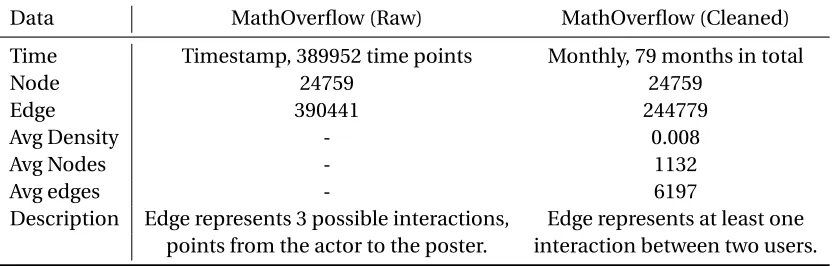
4.4.1 Data Description . . . 57

4.4.2 Data Visualization . . . 58

4.4.3 Real Data Results . . . 61

Chapter 5 Multi-Classes Markov Dynamic Network. . . 63

(9)

5.3 Analysis of MLE . . . 66

5.3.1 Asymptotic Distribution of MLE . . . 67

5.4.1 Settings . . . 74

5.5 Real Data: MovieLens Ratings Network . . . 78

5.5.1 Data Description . . . 78

5.5.2 Data Visualization . . . 79

5.5.3 Determine Class Vectors . . . 84

5.5.4 Real Data Results . . . 85

Chapter 6 Conclusions and Future Directions. . . 89

Bibliography . . . 92

APPENDICES . . . 93

Appendix A Supplementary Materials for Chapter 4 . . . 94

A.1 Parametric Bootstrap of the Dynamic Networks . . . 95

A.2 All-time Bootstrap of the Dynamic Networks . . . 95

Appendix B Supplementary Materials for Chapter 5 . . . 97

(10)

LIST OF TABLES

Table 3.1 Simulation Results for Markov Dynamic Network. For each setting, the dy-namic network is simulated fort : 0→200, and Bootstrapped for 200 times to get the 95% CIs. The estimation results, coverage, variance and the MSE

are then calculated from 500 repeated simulations. . . 25

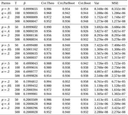
Table 4.1 Simulation Results for FR Model. For each setting, the dynamic network is simulated fort : 0→500, and Bootstrapped for 200 times to get the 95% CIs. The estimation results, coverage, variance and the MSE are then calculated from 500 repeated simulations. Note that the coverage tends to be consistently lower than 95%, which is mainly due to the bias from the network density. . . 55

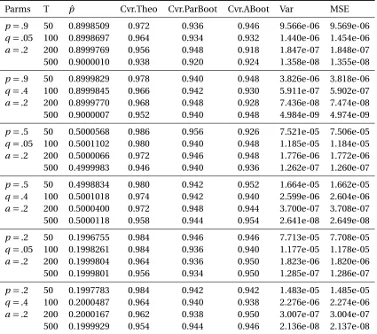
Table 4.2 Simulation Results for RP Model. For each setting, the dynamic network is simulated fort : 0→500, and Bootstrapped for 200 times to get the 95% CIs. The estimation results, coverage, variance and the MSE are then calculated from 500 repeated simulations. Note that the coverage tends to be consistently lower than 95%, which is mainly due to the bias from the network density. . . 56

Table 4.3 MathOverflow Dynamic Network . . . 58

Table 4.4 Results: MathOverflow Interaction Network . . . 62

Table 5.1 Simulation Results: Multi-Classes Markov Dynamic Network . . . 77

Table 5.2 Results: Movies Ratings Dynamic Network . . . 86

Table 5.3 Movies Ratings Dynamic Network: Genres, Year and Rates in each class . . . . 88

(11)

LIST OF FIGURES

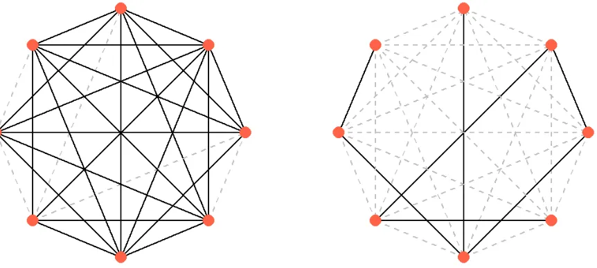
Figure 1.1 Visualization of Two Toy Networks. The solid black line are real edges, while the dash grey line are potential edges. Both networks have 8 nodes in total. The left one is an example of dense network with 23 edges in total. Its nodes’ degrees are{6, 5, 4, 7, 6, 5, 7, 6}. Its density is23₂₈=0.82. The right one is a sparse network with 7 edges. Its nodes’ degrees are{1, 2, 2, 3, 1, 2, 2, 1}. Its density is

7

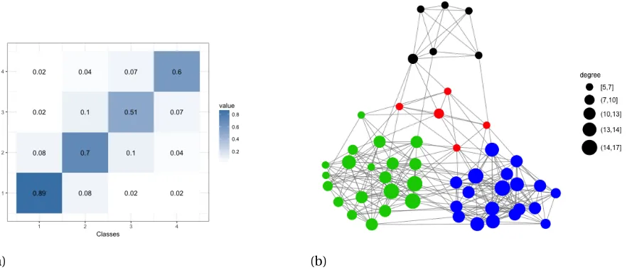
28=0.25. . . 6 Figure 2.1 Visualization of SBM. (a): Heat map of the classes connection probability

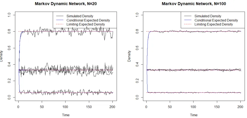
ma-trix. (b): Example of a network generated by SBM using the class connection matrix of the left. . . 11 Figure 3.1 Plots of Network Density from MDN Models with sizesN =20 orN =100.

We can tell from the graphs that the conditional density converge to its limit value shortly. The network density varies around the limit value with larger variation for smaller network size. . . 24 Figure 4.1 Simulated Networks from the RP Model. The size of the node reflects the

number of connections it has. . . 52 Figure 4.2 Behaviors of Network Density for FR Model (above) and RP Model (below).

The probabilities are set to be combinations of the sets:p ∈(0.9, 0.5, 0.2),

q∈(0.4, 0.05), anda=0.2, which corresponds to the limiting densityρ=

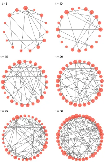
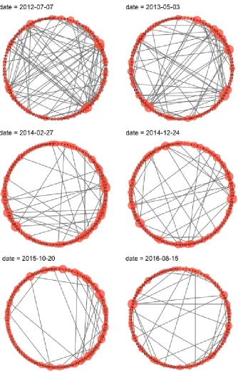
q/(1−p+q)∈ {0.33, 0.80, 0.09, 0.44, 0.06, 0.33}. The initial networks are set to be the same with a density of 0.33. From the plots, we can see that the density of the FR model tends to stable much faster than the RP model. . . . 53 Figure 4.3 MathOverflow Dynamic Network in selected dates. The nodes are placed

in clockwise order from user ID 1 to 100. The size of the node reflects the number of connections it has. . . 59 Figure 4.4 MathOverflow Dynamic Network Monthly Features: The top plot shows that

the number of active users during each time slot. The middle one shows the total interactions (answers to a posted question, comment on a posted question, comment on a posted answer) among users. The bottom plot presents us the trend of network density over time. We can tell clearly that the network grows fast at the beginning, and then tends to stable after about 1 year. . . 60 Figure 5.1 MCMDN Simulation: Plots of Total Nodes and Density over Time. In this

simulation study, we allow nodes to become active and inactive at each time slots. But the number of active nodes will never exceeds the upper bound of 200. . . 76 Figure 5.2 Plots of Movie Rating Network Features. The total movies has a growing trend

but never exceed 415. The network density is high at first, but decreases gradually to around 0.2 at last. . . 79 Figure 5.3 The following two pages show the evolution of MovieLens Ratings Network

(12)

(13)

CHAPTER

1 INTRODUCTION

Network data analysis has become an important branch of statistical science. It originally comes from graphs in mathematics modeling pairwise relations between objects. Agraph, which is denoted byG = (V,E), is basically consist ofverticesandedges, where an edge is a pair of distinct vertices

i,j∈V who are linked. The study of graph model was brought to the statisticians eyes in recent years as there has been an explosion of graph data, and statistical tools are becoming more and more important in analyzing graphs. However, it is more often referred to asNetwork Datain statistical analysis of instead of graph, andnodesinstead of vertices.

(14)

the network effect is never negligible. Game players can be largely affected by their friends or online social medias, especially for group games. In this online game networks, players are considered as different nodes, and the interactions or associations among players are edges. Another application of network model is recommending system. Online merchants or music apps can benefit a lot by building a social network model for their products. In this kind of networks, the products are treated as nodes, the co-buying links among products are edges.

Statistician’s interests on networks mostly lie in analyzing distributions of network metrics, sampling methods of network data, network modeling, network topology inferences and predictions.

Network Characteristics

There has been a great effort on studying the network structure (or graph topology) in mathematics or computer science fields. Such are descriptive tasks that require studying tools much different from statistical tools. Analyzing the distributions of metrics that characterizing network structure looks more statistical. However, different metrics attracts attentions of researchers in different fields. For example, people who study Social Networks may be interested in triangles (small relation circles) of the network.[KC14]breaks the topic of featuring networks into two areas, one focuses on characterizing nodes and edges properties, another focuses on characterizing network cohesion.

An important node-edge features isdegree, which counts the number of edges that connect to a node. Statistical analysis mainly focuses on the degree distribution, which is the distribution of degrees of all nodes in the network, ranging from 0 to total nodes−1. Another frequently referred node-edge feature iscentrality, which characterizes how important a node is in the network. There are multiple way of measuring centrality. One example is theCloseness Centrality, where the node being similar to the most other nodes are consider to be the center.

(15)

has. Theconnectivitymeasures how connective a network is in a global perspective. A connected part is a sub-network where every node is reachable to the other. The networksgroupsis another important feature characterizing network cohesion. It forms an extensive discussion about the network partition methods including hierarchical clustering and spectral analysis.

Sampling Methods

When it is impossible or too expensive to observe the entire network, sampling is necessary. However, due to the special structure of network data, it differs a lot from traditional statistical sampling. An intuitive way is random sampling pure nodes or edges first, then the related edges among sampled nodes or the nodes connected to the sampled edges are then taken directly from the network. Such ways re referred to asInduced or Incident Sampling. Another sampling method isStar Sampling, which just as its name implies, samples the nodes and its induced edges, together with the nodes connected to the edges. An extension to the star sampling isSnowball Sampling. It samples the nodes, their induced edges, then the incident nodes and their induced edges continuously like rolling a snowball until theKth stage.

When sampled network data is available, the traditional statistical inference theories are used to estimate the network properties.

Network Models

Much of statistical work on network data is focusing on modeling. This topic of work falls in a number of important classes. Some is network motifs. Among those is the fundamental model,

Random Graph Modeloriginally proposed by[ER59], where edges are placed between pairs of nodes

identically and independently with a fixed probabilityp. Later models such asStochastic Blockmodel

andLatent Space Modelare based on the random graph model. TheExponential Random Graph

Modelis also a generalization of the random graph models. However, it generalizes the independence

(16)

Models. This kind of models are mostly used on dynamic networks, which address the changing of network structure in time. Such models are first proposed in describing the growth of World Wide Web. They are also widely used in biological sciences. ThePreferential Attachment Modelsand

Copying Modelsare typical network growth models.

Inferences and Predictions

Once the data and model are constructed, the key work falls on estimation of model parameters and prediction on unknown network structures. Our work in this paper mainly focuses on modeling and inferring on dynamic networks. Then real data are applied and predictions on the data are made based on proposed model and estimations.

1.1 Notations

Typically, we useG(V,E)to refer to a network graph in statistical modeling, whereV ={1, ...,n}

stands for the vertices(nodes) set, andE stands for the edges set. The superscriptt is added when studying dynamic network graph models. That is,G(Vt_,_Et₎_{stands for the dynamic network status} at timet. The link structure of a network is represented by an adjacency matrix:

X=



      

0 X₁₂ . . . X1n

x11 0 . . . X2n ..

. ... ... ...

xn1 xn2 . . . 0



      

.

In this paper, we only talk about undirected, unweighted network, where the adjacency matrix is symmetric with 0’s on the diagonal, and 0 or 1 off diagonal. IfX_{i j}=1, it stands that nodesi andj

are connected. Otherwise, they are not connected.

(17)

snapshott.

The node degreedi=

P

j∈V Xi j counts the number of edges that are connected to nodesi. In an directed network,di can be divided todii nanddio u t, wherei n stands for edges pointing towardi,

ando u t stands for edges pointing fromitowards other nodes. The citation network is an example

of directed network, where the edges point from the paper to the cited one. Our models discussed in later chapters are undirected networks. Such includes friendship network, where the node degree is simply the number of friends of a personi. The degree distribution of a network is the distribution of the series{d1, ...,dn}. It describes how connective among nodes the network is.

The Network Growth Model is one kind of models which bases the evolution mechanism on the degree distribution. The Preferred Attachment mechanism adds new node with degreed≥1. The Copying mechanism adds a new node to the existed network with randomly chosen edges of a randomly chosen existed node. Both mechanism grow the network to a power-law degree, which suggests that the degree distribution

f(d)∝d−α.

The network density, which is denoted by

ρ= |E|

|V|(|V| −1)/2,

is basically the total edges divided by total potential edges, describes how dense the network edges are. A visualization of two toy networks with different densities are show in Fig.1.1.

1.2 Organizations

The paper is organized as follows. Chapter 2 are literature reviews on existing famous network models and existing estimation methods of those models.

(18)

Figure 1.1Visualization of Two Toy Networks. The solid black line are real edges, while the dash grey line are potential edges. Both networks have 8 nodes in total. The left one is an example of dense network with 23 edges in total. Its nodes’ degrees are{6, 5, 4, 7, 6, 5, 7, 6}. Its density is23₂₈=0.82. The right one is a sparse network with 7 edges. Its nodes’ degrees are{1, 2, 2, 3, 1, 2, 2, 1}. Its density is₂₈7 =0.25.

before, then the edge variable follows Bernoulli(p), otherwise, Bernoulli(q). This model assumes that all edges follow the same pattern across the whole network, which is usually not the case in reality. Then, we give Maximum Likelihood Estimators for the parameters and analyze the limiting distribution of the estimators by applying Martingale Central Limit Theorem.

In Chapter 4, We look into a more general case where the network size is growing over time. We provide two models: one assumes that nodes coming in a constant rate, the other is a more generalized that assume node come and leave in Poisson distributions with coming rate larger than leaving rate. Consequently, The network size grows to infinity as time goes to infinity. Asymptotic distributions are provided for the MLE of the models. Simulation results are then provided for the estimation of the Growing Size Models.

(19)

cases, in dynamic cases, the group memberships vary in time. We model the group membership with a random class vector for each nodes as the function of linkages at the former time. Thus forms a Markov Chain.

1.3 Summary of Results

We have shown that for the base model, Markov Dynamic Network:

1. The network tends to be dynamic stable;

2. The Markov chain formed by the edges is irreducible and ergodic. The status 0 and 1 are recurrent;

3. The asymptotic distribution of the maximum likelihood estimator normal with a constant variance that is the function of the keeping probabilitypand appearing probabilityq. The convergence rate isT.

For the second model, Fixed rate Markov Dynamic Network, and its generalized model, Random Process Markov Dynamic Network, we have shown that:

1. The network density goes in probability to a constant function of the parameters. To be specific, the limiting network density is ₁₋_pq₊_q under both models. The limiting density is independent of the how node come into or leave the network;

2. The asymptotic distribution of MLE for keeping probabilitypand appearing probabilityq

are normal with a constant variance that is the function ofp andq. That for the forming probabilityais normal with a constant variance of function ofaonly. The convergence rate isT3;

(20)

Finally, for the third model, Multi-Classes Markov Dynamic Network, we get the following results:

1. The network tends to be dynamic stable. The Markov Chain formed by the vectorized adjacency matrix has an unique stationary distribution;

2. The MLE is asymptotically normal with convergence rate ofT;

(21)

CHAPTER

2 LITERATURE REVIEWS

2.1 Existing Network Models

Network models has been widely studied by researchers for dealing with relational data in sociology, technology and biology. The Random Graph Model for static networks addresses the randomness of edges, but ignores the diversity of nodes. To solve this issue,[Hol83]proposed a new model called Stochastic Block model (SBM), where nodes are assigned into different blocks, and those from the same block are considered statistically the same. More specifically:

(22)

least one node in each class). Then

P(X_{i j}=1|c_i,c_j) =E(X_{i j}|c_i,c_j),

where ciis the i th row of class matrix C . Then, the Stochastic Blockmodel satisfies that

E(X|C) =C B CT,

where B∈[0, 1]k×kis the class connection probability matrix which is full rank and symmetric.

Figure 2.1 shows an example network generated from the Stochastic Blockmodel with 4 blocks (classes). The class connection probability matrix is shown in the heat-map in (a), where we can tell that the within-group connection probability is much higher than the between-group connection probability. The network generated is shown in (b). The color of the nodes stands for the group the nodes belong to. It can be seen easily that nodes are closely connected if they belong to the same group. The estimation of the SBM mainly includes two steps: 1. grouping of nodes using the adjacency matrix; 2. Estimation of the class connection matrix. The first step shows its importance in the estimation of SBM and we will discuss it later.

A more general model, Latent Space Model (LSM), is proposed by[Hof02]to describe social network, where the edge probability depends on the "positions" of nodes in an unobserved "social space".

Definition 2.1.2. (Latent Space Model)Suppose X ∈ {0, 1}n×n_{is the adjacency matrix of a random}

network with n nodes. Define Z ∈ Rn×k is the latent space matrix such that the row vectors are

independent inRk. Assume that a probability distribution on X has conditional independence

relationship

P(X|Z) =Y

i<j

P(Xi j|zi,zj),

(23)

(a) (b)

Figure 2.1Visualization of SBM. (a): Heat map of the classes connection probability matrix. (b): Example of a network generated by SBM using the class connection matrix of the left.

where ziis the i th row of latent space matrix Z . Then, it is an undirected Latent Space Model. The

Stochastic Blockmodel is a special case of Latent Space Model with the latent space matrix Z =C .

To be specific, the probability of an edge in a LSM are determined by the latent distance between two nodes, which is determined by the latent vectorsZi. Likelihood-based method can be used to estimate the latent distances and thus the latent vectors once the distance structure is defined.

It should be brought into consideration that under many situations, the networks are time-varying. In recent years, dynamic networks has drawn more and more attention of researchers. [Han15]view dynamic network as multi-layer graphs, and the multi-graph SBM is analyzed with an exploration of the asymptotic properties of spectral clustering estimator and the maximum likelihood estimate (MLE).

(24)

where Bt ∈[0, 1]k×k is the class connection probability matrix at time layer t which is full rank and symmetric.

However, this multi-layer model ignores the time scale relationships between the "layers". Another limitation is the assumption that block structure is fixed overtime. This is not true in many real situations when nodes may switch classes. In addition, The class connection probability matrix is changing overtime, making the number of parameters grows linearly as time evolves. This may add to the computation time greatly.

Later works regarding dynamic stochastic block model mainly focus on block detection and clustering of the nodes.[MM17]proposed a clustering method on estimating time related Stochastic Blockmodel, which allows class switching across time while assuming that most of the nodes do not change classes across two different time steps. Furthermore, they assume the class vector

Ci={Cit}0≤t≤Tto be an irreducible, aperiodic stationary Markov chain with a stationary distribution. Conditional onCt, the distribution of adjacency matrixXt follows a Stochastic Blockmodel with the class connection probability matrix varying across time.

[Zha17a]addresses the time scale interaction of networks, and generalizes some standard net-work models with the assumption that the presence and absence of edges are governed by Markov processes. A blockmodel based dynamic network is also introduced, where one assumes that the appearance and disappearance of edges are governed by continuous-time Markov processes. Those probabilities are depend on an rate parameters that can depend on properties of the nodes. The parameters can be estimated from the adjacency matrix using likelihood based methods. They provide some algorithm for achieving the MLE, but the analysis of the asymptotic properties of the estimators is not included. One of our tasks is to analyze the long time behaviors of the networks under different dynamic models, and then give an asymptotic distribution of MLE.

(25)

network and form relationships with the existing ones. Another example is when studying the long-time interaction of students in a college, the entering of new students and leaving of graduating students should also be considered. We give an discussion about a generalization of the Markov Dynamic Network by allowing the continuous coming of new nodes, with the assumption that existed nodes do not disappear at all.

2.2 Existing Model Estimation Methods

Non-parametric graphon estimations has been proposed by[WO13]for estimating kernel-based network models. The graphon is non-negative symmetric, measurable and bounded function that represents a discrete network as an infinite-dimensional analytic object. It can be viewed as a heat map of the expected adjacency matrix independently of the network size. Usually a graphonf(x,y)

is defined on(0, 1)2_{. Each node}_i_{will be mapped uniformly onto a position on}_ξ

i∈(0, 1)identically. Then the edge probabilitypi j can be specified by

pi j=ρnf(ξi,ξj), {ξ1, ...,ξn} i.i.d.

∼ Uniform(0, 1), ∫ ∫ f(x,y)d x d y=1.

It is stated that this graphon function is unique in the exchangeable sense. In estimating the graphon, the basic method is approximating the function by class connection probability matrix in Stochastic Blockmodel. Once the nodes are grouped, they are permuted such that those in the same group are in neighbour positions. The last step is fitting a block model, and the estimated class connection probability matrix is a discretized approximation of the graphon function.

A famous method in estimating the node classes is using spectral clustering of the adjacency matrix proposed by[Roh11]. For a given network adjacency matrixX_n_×_nwhere the diagonals are zeros, define matrixLn×nas

L=D−1/2X D−1/2,

(26)

a) Find out the eigenvectors corresponding to the firstklargest absolute eigenvalues of matrix

L. Use thek vectors to form an eigenmatrixEn×k.

b) Treat each rowiof the matrixE as position of nodeiin the spaceRk. Use k-means clustering to group the rows. Output the class of rowias the class of nodei.

Such clustering is efficient and has wide usage with little assumptions. The idea behind this method is that the largestk eigenvectors expressed thekmain directions of the whole adjacency matrix in a

n×nspace. The nodes points to the similar directions are more likely to be grouped into the same class.

[Zha17b]proposed a neighbourhood smoothing method on estimating the class connection probability matrix. They define a nodeâ ˘A ´Zs neighborhood to consists of nodes with similar rows in the adjacency matrix. However, this method requires much more computation than the spectral method, though it shows comparable estimation results.

2.3 Convergence Theorems for Markov Chains

[AL06]gives the definition of Markov Chain in countable state space and some of important proper-ties as follows.

Definition 2.3.1. (Markov Chain in countable State Space)Suppose{Xt}Tt=0is a series of random

variables on probability space(Ω,F,P). The state spaceS ={i1, ...,iK},K <∞is countable. If

• P(X0=ik) =µk,∀k ;

• P(Xt+1=ib|Xt =ia,Xt−1=iat−1, ...,X0=ia0) =pa b∀ia,ib,iat−1, ...,ia0∈ S and t =0, 1, 2, ...,T . Then{Xt}Tt=1is Markov Chain with stationary probabilityP= (pa b), initial distributionµ, and state

spaceS.

Definition 2.3.2. (Irreducibility)The transition probabilityP= (pa b)of a Markov Chain is called

(27)

Definition 2.3.3. (Recurrence)The state i of a Markov Chain is called recurrent if P(Ti <∞) =1,

where Tiis the hitting time of state i , which is the first time after 0 that the chain enters i . Furthermore,

a recurrent state i is called positive recurrent ifEi(Ti)<∞.

The basic ergodic theorem and its proof is then given in the[AL06].

Theorem 2.3.1. (Basic Ergodic Theorem)Suppose a Markov Chain with countable state spaceS has transition probabilityP. The transition probability is irreducible, let one state to be positive recurrent, then

1. All states are positive recurrent;

2. There exists a stationary probabilityπ;

3. For any initial probability, and any state i ∈ S,

• _T1₊₁PT

t=0P(Xt =j)→πj;

• L_t(j) =_T1₊₁PT

t=0δ(Xt=j)→pπj, where Lt(j)is the empirical distribution at t .

2.3.1 Martingale CLT

[AL06]introduces Martingale CLT that is useful in the analysis of estimators in our models. First, the concept of Martingale Difference Array (MDA) is introduced.

Definition 2.3.4. Let(Ω,F,P)be a probability space. Let{Xi}ni=1be r.v.s on(Ω,F,P), and{Fi}ni=1

be subσ-fields ofF.

1. IfFi⊂ Fi+1,∀i=1, 2, ...,n , thenFiis called a filtration.

2. {Xi}n_i₌₁is called a Martingale Difference Array if

• XiisFi-measurable,∀i=1, 2, ...,n .

(28)

Then, it is easy to introduce Martingale Central Limit Theorem. We will use the Martingale CLT in Chapter 3-5 to prove the consistency and asymptotic normality of the estimators.

Theorem 2.3.2. (Martingale CLT)For n≥1, let{Xi}ni=1be an MDA with respect to{Fi} n

i=1such that

1

n

X

i=1

E(X_i2|Fi−1)

p

−→σ2_∞∈(0,∞),

and one of the following

• Lindeberg’s Condition:∀ε >0,

1

n

X

i=1

E(X_i21(|Xi|> ε)|Fi−1)

p

−→0as n→ ∞;

• Lyapunov’s Condition:

1

n

X

i=1

E(X_i4|Fi−1)

p

−→0as n→ ∞,

is satisfied. Then,

1

n

X

i=1

Xi p

(29)

CHAPTER

3 MARKOV DYNAMIC NETWORK

3.1 Model Settings

[Zha17a]proposed 3 dynamic network models, including dynamic random graph model, the dy-namic random graph with arbitrary expected degrees and the dydy-namic block model. The first model proposed was defined after the classical random graphG(n,p)studied by[ER59]. This model de-scribes the varying of the network by adding an edge to the previously disconnected nodes with probabilityα, or not with probability 1−α. Similarly, the model deletes the edge between the previ-ously connected nodes with the probabilityβ, or not with probability 1−β. And at the starting time pointt =0, it is a random graphG(n,p).

(30)

t =1, 2, ...,T. Then

X_{i j}t =X_{i j}t−1◦Bt+ (1−X_{i j}t−1)◦Ct, (3.1)

where Bt _∼_Bern(_p₎_and_Ct _∼_Bern(_q₎_{are Bernoulli random variables at time}_t _{(Assume i.i.d.).} We have assumed that the initial distribution is nonrandom. In addition, we assume thatX_{i j}t are independent with respect to the indexi < j, i.e., the edges are independent with each other for different nodes pairs.

Although[Zha17a]has given the Maximum Likelihood Estimator, the properties of the estimators have not been studied yet. Our goal in this chapter is mainly extending their work by studying the behavior of the MLE asT → ∞of the model.

3.2 Markov Properties

3.2.1 Irreducibility, Ergodicity and Recurrence

From equation 3.1, it is easy to have that{X_{i j}t :t ≥0}is a Markov Chain on a state space ofS={0, 1}, with the transition probability matrix

P =





1−q q

1−p p 

, lim

T→∞P

T₌





1−p 1−p+q

q 1−p+q 1−p

1−p+q q 1−p+q



,

Thus the invariant probabilityπ= (₁₋1−_pp₊_q,₁₋_pq₊_q). In addition, the eigenvalues of matrixP are 1 and

p−q, and the corresponding eigenvectors are(1, 1)0_and₍₋_q_{, 1}₋_p₎0_{. Using the eigen-decomposition,}

we have

P =U





1 0

0 p−q 

U−1⇒ Pn=U 



1 0

0 (p−q)n 

U−1,

where,

U =





1 −q

1 1−p 

, U−1= 



1−p 1−p+q

q 1−p+q

−1

1−p+q 1 1−p+q



(31)

First, since the 1-step transition probabilities of 0→1, and 1→0 arep00=1−q>0 andp11=p>0 respectively, the chain isirreducible, and thusergodic. Second, then-step transition probabilities of 0→1, and 1→0 are

p₀₀(n)= 1−p

1−p+q + q

1−p+q(p−q)

n_,

p₁₁(n)= q

1−p+q +

1−p

1−p+q(p−q)

n_.

Hence, states 0 and 1 arerecurrent, as

lim

n→∞E0Nn(0) = ∞ X

n=1

p₀₀(n)= ∞ X

n=1

1−p

1−p+q+ q

1−p+q(p−q)

n

=∞,

lim

n→∞E1Nn(1) = ∞ X

n=1

p₁₁(n)= ∞ X

n=1

q

1−p+q+

1−p

1−p+q(p−q)

n

=∞.

Furthermore, they arepositive recurrentsince

lim

n→∞E0Ln(0) =nlim→∞

1

n

X

k=1

p₀₀(k)= 1−p

1−p+q >0,

lim

n→∞E1Ln(1) =nlim→∞

1

n

X

k=1

p₁₁(k)= q

1−p+q >0.

From[AL06]Theorem 14.1.16,(S,P)is irreducible and state 0 and 1 are positive recurrent. Thus,

1

T

X

t=1

(1−Xt) =L_T(0) = 1 T

T

X

t=1

δ{Xt =0}−→p π0= 1−p

1−p+q, (3.2)

1

T

X

t=1

Xt =LT(1) = 1

T

X

t=1

δ{Xt=1}−→p π1=

q

(32)

3.3 Model Estimation

3.3.1 Maximum Likelihood Estimators The likelihood ofp andqgivenXt andXt−1is

L_t(p,q|X_t,X_t₋1) =Y

i<j

pxi jt (1₋_p)1−x t i jx

t−1

i j _qxi jt (1₋_q)1−x t i j1−x

t−1

i j _.

Then the likelihood ofpandqgiven{X₀,X₁, ...,X_T}is

L(p,q|X0, ...,XT) = T

Y

t=1

Y

i<j

pxi jt (₁₋_p)1−xi jt x t−1

i j

qxi jt(₁₋_q)1−xi jt 1−x t−1

i j _.

Take the log and we get

l(p,q|X0, ...,XT) = T

X

t=1

X

i<j

x_{i j}t−1x_{i j}t lnp+x_{i j}t−1(1−x_{i j}t )ln(1−p)

+ (1−x_{i j}t−1)x_{i j}t lnq+ (1−x_{i j}t−1)x_{i j}t ln(1−q), ∂l

∂p =

1

p

T

X

t=1

X

i<j

x_{i j}t−1x_{i j}t − 1

1−p

T

X

t=1

X

i<j

x_{i j}t−1(1−x_{i j}t ),

∂l

∂q =

1

q

T

X

t=1

X

i<j

(1−x_{i j}t−1)x_{i j}t − 1

1−q

T

X

t=1

X

i<j

(1−x_{i j}t−1)(1−x_{i j}t ).

Set the partial derivative to 0, we get the maximum likelihood estimator forp andqas

ˆ

pM L E =

PT t=1

P

i<j xi jt−1xi jt

PT

t=1

P

i<jxi jt−1 =

P

i<j

PT

t=1xi jt−1xi jt

P

i<j

PT

t=1xt−1

, (3.4)

ˆ

q_{M L E} = PT

t=1

P

i<j(1−xi jt−1)x t i j

PT

t=1

P

i<j(1−xi jt−1) =

P

i<j

PT

t=1(1−x t−1 i j )x

t i j

P

i<j

PT

t=1(1−x t−1 i j )

(33)

3.3.2 Asymptotic Distribution of MLE

Theorem 3.3.1. Let{X_{i j}t }t>0defined on(Ω,A,P)follows the Markov Dynamic Network model,

assuming that the initial network is nonrandom, then the MLE of keeping probability p is consistent

and the asymptotic distribution

v

tT n(n−1)

2 (pˆM L E −p) d

−→N0,p(1−p)(1−p+q)

q

. (3.6)

The MLE of appearance probability q is consistent and follows

v

tT n(n−1)

2 (qˆM L E−q) d

−→N0,q(1−q)(1−p+q) 1−p

. (3.7)

As the proof of form (3.7) is quite similar to the proof of form (3.6), we will only show the proof of form (3.6), the proof of the other is omitted.

Proof. From the large number result we got in form (3.3), we have

1

T

X

t=1

X_{i j}t −→p π1=

q

1−p+q.

As the edges are i.i.d.,

2

T n(n−1) X

i<j T

X

t=1

X_{i j}t −→p π1=

q

1−p+q.

Now let

Y_{i j}t =X_{i j}t−1X_{i j}t

=X_{i j}t−1(X_{i j}t −p) +p X_{i j}t−1

(34)

Then

ˆ

pM L E =

P

i<j

PT

t=1xi jt−1xi jt

P

i<j

PT

t=1x t−1 i j

=

P

i<j

PT t=1zi jt

P

i<j

PT

t=1x t−1 i j

+p.

LetFa =σ〈Xt :t ≤a,t ∈Z〉,−∞ ≤a≤b≤ ∞. AsXi jt are i.i.d. for eachiand j, we leave out the subscripti,jfor simplicity.

Now we show thatZt _{is MDA. First, it is easy to see that}_Zt _is_F

t-measurable,∀t =1, 2, ...,T. Then, for allt,

E(Zt|Ft−1) =E

Xt−1(Xt−p)Xt−1,Xt−2, ...,X0

=Xt−1EXt−pXt−1,Xt−2, ...,X0

=Xt−1Xt−1p+ (1−Xt−1)q−p

=

(Xt−1)2−Xt−1(p−q)

=0.

ThusZt is MDA. In addition, the conditional variance ofZt is

σ2 t=E

(Zt)2F_t₋₁

=EXt−1(Xt−p)2Xt−1,Xt−2, ...,X0

= (Xt−1)2E(Xt)2−2p Xt+p2Xt−1,Xt−2, ...,X0

=Xt−1E(1−2p)Xt+p2Xt−1,Xt−2, ...,X0

=Xt−1(1−2p)(Xt−1p+ (1−Xt−1)q) +p2

=p(1−p)Xt−1.

From form (3.3), we get

1

T

X

t=1 σ2 t = 1 T T X

t=1

p(1−p)Xt−1−→p p q(1−p)

(35)

At last,

1

T

X

t=1

E(Zt)21(|Zt|> εpT)F_t₋₁

≤ 1 T

T

X

t=1

E1(|Zt|> εpT)F_t₋₁

→0 asT → ∞.

Therefore, we have the limiting distribution ofZ_{i j}t as

1

p T

T

X

t=1

Z_{i j}t −→d N0,p q(1−p) 1−p+q

.

As{Z_{i j}t }are i.i.d for eachi,j, and by Slutsky’s Theorem,

v

tT n(n−1)

2 (pˆM L E−p) =

v

tT n(n−1)

2

P

i<j

PT t=1Zi jt

P

i<j

PT

t=1X t i j

d

−→N0,p(1−p)(1−p+q)

q

. (3.8)

3.4 Simulation Study

3.4.1 Settings

In our simulation studies for MDN model, the networks are generated with sizesN ∈(20, 100), and

initial edge probability of 1/3. The total time we run for the dynamic network is 500. The keeping probabilityp, appearing probabilityqare set to be combinations ofp∈(0.9, 0.5, 0.2),q∈(0.4, 0.05). Figure 3.1 shows the change in network density over time for each settings.

3.4.2 Simulation Results

(36)

Figure 3.1Plots of Network Density from MDN Models with sizesN=20 orN=100. We can tell from the graphs that the conditional density converge to its limit value shortly. The network density varies around the limit value with larger variation for smaller network size.

relatively small compared to the true parameter.

(37)

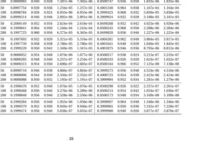
Table 3.1Simulation Results for Markov Dynamic Network. For each setting, the dynamic network is simulated fort : 0→200, and Boot-strapped for 200 times to get the 95% CIs. The estimation results, coverage, variance and the MSE are then calculated from 500 repeated simulations.

Settings T pˆ Cvr.T Cvr.B Var MSE qˆ Cvr.T Cvr.B Var MSE

n=20 50 0.9001018 0.960 0.960 2.548e-05 2.544e-05 0.0501229 0.954 0.930 7.129e-06 7.130e-06 p=.9 100 0.9001643 0.940 0.934 1.473e-05 1.473e-05 0.0500193 0.934 0.918 3.917e-06 3.910e-06 q=.05 200 0.9000983 0.940 0.928 7.307e-06 7.302e-06 0.0500747 0.956 0.950 1.833e-06 1.835e-06

(38)

CHAPTER

4 GROWING SIZE MARKOV DYNAMIC

NETWORK

In this chapter, we introduce the Growing Size Dynamic Network Model (GSMDN). In this model, we no longer assume that the total number of nodes stays the same over time. Instead, we allow the network size to be changeable.

4.1 Base Model: Fixed Rate Model

4.1.1 Model Settings

(39)

Suppose the original network size isn0. Then the network size at timet isnt =n0+t.

It should be noticed that the appearing probability between old nodes is different from the one related with new coming node. For example, in social network, People are more likely to keep their old relationship than forming a friendship with new comer. In addition, people tend to trust more on the users who entered in earlier than on the new comers. Now letabe the probability with respect to the new node, which is called the forming probability in this paper. Now, in the FR model, the keeping probability, appearing probability and forming probability are

P(X_{i j}t =1|X_{i j}t−1=1) =p, ifi,j∈Vt−1,

P(X_{i j}t =1|X_{i j}t−1=0) =q, ifi,j∈Vt−1,

P(X_{i j}t =1|X_{i j}t−1=0) =a, ifiis the new coming node,j∈V_t₋₁.

4.1.2 Behavior of the Network Density

LetL_t be the total edges at timet. The expected edges at timet is E(L_t) =l_t. Then suppose at time

t +1, the expected edges that still keep should beLtp. Expected number of new edges form where there is no edge at timet is[nt(nt−1)/2−Lt]q. As for the new coming node, there arent new pair of nodes that could potentially form an edge in between. Thus expected new edges coming along with the new node isnta. The expected total edges at timet+1 is

l_t₊₁=E(L_t₊1)

=EE(Lt+1|Lt)

=E¦Ltp+

n_t(n_t−1)

2 −Lt

q+nta

©

=E(Lt)(p−q) +

nt(nt−1)

2 q+nta =lt(p−q) +

nt(nt−1)

(40)

Note thatnt(nt−1)

2 is the potential edge number at timet. According to the definition of network density%t=nt(2Lntt−1), we have the expected network densityρt=E(%t)as below:

n_t(n_t+1)ρ_t₊₁=n_t(n_t−1)ρ_t(p−q) +n_t(n_t−1)q+2n_ta. (4.1)

Equation (4.1) can be seen as a recursion formula for calculating the expected density. Now let

bt = (nt−1)ntρt+c0nt2+c1nt+c2.

We should find some constantsc0,c1,c2to satisfy that

bt =bt−1(p−q).

Solve forbt we have

bt =b0(p−q)t,

which can also be written as

(nt−1)ntρt+c0nt2+c1nt+c2=

(n0−1)n0ρ0+c0n02+c1n0+c2

(p−q)t.

Solve forρt we have

ρt =

(p−q)t

(nt−1)nt

(n0−1)n0ρ0+c0n02+c1n0+c2

− c0nt nt−1−

c1

nt−1−

c2 (nt−1)nt

.

From the expression forρt, we can get

lim

(41)

Now we solve forc0,c1,c2. Compare

n_t(n_t+1)ρ_t₊₁+c0(n_t+1)2+c1(n_t+1) +c₂= [(n_t−1)n_tρ_t+c₀n2_t+c₁n_t+c2](p−q).

with equation (4.1), we have

(p−q−1)c₀=q,

(p−q−1)c1−2c0=2a−q, (p−q−1)c2−c0−c1=0.

Thus we get

c₀= q

p−q−1,c1=

2c0+2a−q

p−q−1 ,c2=

c0+c1

p−q−1, (4.2)

which leads

lim t→∞ρt =

q

1−p+q.

Now we look at the limit variance of%t. First, we have

Var(%t+1) =_n2 4 t(nt+1)2

Var(Lt+1)

= 4

n_t2(nt+1)2

E(Var(Lt+1|Lt)) +Var(E(Lt+1|Lt))

,

and

E(Var(Lt+1|Lt)) =E

p(1−p)Lt+q(1−q)

n_t(n_t−1)

2 −Lt

+a(1−a)nt

=E(Lt)

p(1−p)−q(1−q)+q(1−q)nt(nt−1)

2 +a(1−a)nt, Var(E(L_t₊₁|L_t)) =Varp L_t+qnt(nt−1)

2 −Lt

+a n_t

(42)

Thus,

Var(%t+1) = 4

n_t2(nt+1)2

¦

E(L_t)p(1−p)−q(1−q)+q(1−q)nt(nt−1)

2 +a(1−a)nt+Var(Lt)(p−q)2

©

= 2(nt−1)

nt(nt+1)2 E(%t)

p(1−p)−q(1−q)+ 2(nt−1) nt(nt+1)2

q(1−q)

+ 4

nt(nt+1)2

a(1−a) +(nt−1)

2 (nt+1)2

Var(%t)(p−q)2.

Take the limit on both sides, we have

lim

t→∞Var(%t+1) = (p−q)

2 _lim

t→∞Var(%t).

As

Var(%_t) =

E(%2_t)−E2(%_t) <

E(%2_t)

+

E2(%_t)

<2<∞,

we get

lim

t→∞Var(%t) =0.

Thus we can easily have the following lemma about%t.

Lemma 4.1.1. Suppose the FR model. Let Lt be the total edges at time t, and%t = _n_t2L₍_n_tt₋₁₎ be the

network density at time t , where nt=n0+t is the network size at time t . The expected network density

isρt =E(%t), then we have

lim

t→∞E(%t) = q

1−p+q, limt→∞Var(%t) =0.

Thus

%t p

−→ q

(43)

Furthermore,

6

T3 T

X

t=1

Lt = 6

T3 T

X

t=1

nt(nt−1)%t 2

p

−→ q

1−p+q. (4.3)

Proof. The proof of the lemma is straightforward from the above analysis of network density. Then

asn_t =n₀+t, the proof of form (4.3) comes directly from law of large numbers.

Note that the limit ofρt does not depend on the appearing probabilityafrom new coming node. Actually, as long as the number of nodes coming at a time is finite, the limit ofρt will not depend on

a.

4.1.3 Analysis of MLE

The Likelihood function is:

L(λ,θ|X0, ...,XT) =

T

Y

t=1

¦ Y

i,j∈Vt−1,i<j

pxi jt (₁₋_p)1−xi jtx t−1

i j Y

i,j∈Vt−1,i<j

qxi jt (₁₋_q)1−xi jt1−x t−1

i j

× Y

i,j∈Vt

where Vt stands for the vertex (nodes) set at time t, and Xt = {Xi jt ,i < j,i,j ∈ Vt}.Vt = {i ∈

Vt\Vt−1,j∈Vt−1} ∪ {j∈Vt\Vt−1,i∈Vt−1} ∪ {i,j∈Vt\Vt−1,i<j}denotes the set that eitherior jis the new comers at timet. Take the log of the likelihood and let the first derivative to 0, we can get the MLE as below:

ˆ

pM L E=

PT

t=1

P

i<j,i,j∈Vt−1X

t−1 i j Xi jt

PT t=1

P

i<j,i,j∈Vt−1X

t−1 i j

, (4.4)

ˆ

qM L E=

PT t=1

P

i<j,i,j∈Vt−1(1−X

t−1 i j )Xi jt

PT

t=1

P

i<j,i,j∈Vt−1(1−X

t−1 i j )

, (4.5)

ˆ

aM L E=

PT

t=1

P

i,j∈VtX t i j

PT

t=1

P

i,j∈Vt1

. (4.6)

(44)

a are consistent and have asymptotic distributions as

v tT3

6 (pˆM L E −p) d

−→N0,p(1−p)(1−p+q)

q

, (4.7)

v tT3

6 (qˆM L E−q) d

−→N0,q(1−q)(1−p+q) 1−p

, (4.8)

v tT2

2 (aˆM L E−a) d

−→N(0,a(1−a)). (4.9)

Proof. Since the proofs of (4.8) and (4.9) are quite similar to that of (4.7), we only prove for (4.7) here. Let

Zt=

X

i<j,i,j∈Vt−1

X_{i j}t−1(X_{i j}t −p).

Then

ˆ

p_{M L E} = PT

t=1

P

i<j,i,j∈Vt−1X

t−1 i j X

t i j

PT

t=1

P

i<j,i,j∈Vt−1X

t−1 i j

=

PT t=1Zt

PT

t=1Lt−1 +p.

First, for the denominator

D=

T

X

t=1

Lt−1,

we have proved in Lemma. 4.1.1 that

6

T3 T

X

t=1

Lt−1 p

−→ q

(45)

Now letFa=σ〈Xt :t ≤a,t ∈Z〉,−∞ ≤a≤b≤ ∞, we showZt is MDA.

E(Z_t|Ft−1) =E

X

i<j,i,j∈Vt−1

X_{i j}t−1(X_{i j}t −p) X

t−1

= X i<j,i,j∈Vt−1

X_{i j}t−1E X_{i j}t −pXt−1

= X i<j,i,j∈Vt−1

X_{i j}t−1 X_{i j}t−1p+ (1−X_{i j}t−1)q−p

= X i<j,i,j∈Vt−1

X_{i j}t−1 X_{i j}t−1p+ (X_{i j}t−1−X_{i j}t−1)q−X_{i j}t−1p

=0,

whereXt stands for{X_{i j}t ,i<j,i,j∈Vt}. AsXi jt−1are 0 or 1, we haveXi jt−1= (Xi jt−1)2. In addition,

E(Z_t2|Ft−1) =E

X

i<j,i,j∈Vt−1

X_{i j}t−1(X_{i j}t −p)2 X

t−1

= X i<j,i,j∈Vt−1

(X_{i j}t−1)2E(X_{i j}t −p)2Xt−1

+ X i<j,i,j∈Vt−1

X

k<l,k,l∈Vt−1,(k,l)6=(i,j)

X_{i j}t−1X_{k l}t−1E(X_{i j}t −p)(X_{k l}t −p)Xt−1

=I+II.

First,

I= X

i<j,i,j∈Vt−1

(X_{i j}t−1)2E(X_{i j}t )2−2p X_{i j}t +p2Xt−1

= X i<j,i,j∈Vt−1

X_{i j}t−1E(1−2p)X_{i j}t +p2Xt−1

= X i<j,i,j∈Vt−1

X_{i j}t−1(1−2p)(X_{i j}t−1p+ (1−X_{i j}t−1)q) +p2

= X i<j,i,j∈Vt−1

X_{i j}t−1(1−p)p

(46)

whereLt is the number of edges at timet. Second,

II= X i<j,i,j∈Vt−1

X

k<l,k,l∈Vt−1,(k,l)6=(i,j)

X_{i j}t−1X_{k l}t−1E(X_{i j}t −p|Xt−1)E(X_{k l}t −p|Xt−1)

=X XX_{i j}t−1X_{i j}t−1p+ (1−X_{i j}t−1)q−pX_{k l}t−1X_{k l}t−1p+ (1−X_{k l}t−1)q−p

=X X X_{i j}t−1p+ (X_{i j}t−1−X_{i j}t−1)q−X_{i j}t−1pX_{k l}t−1p+ (X_{k l}t−1−X_{k l}t−1)q−X_{k l}t−1p

=0.

Thus,

E(Z_t2|Ft−1) = (1−p)p Lt−1.

Again, use Lemma. 4.1.1, we have

6

T3E(Z 2 t|Ft−1)

p

−→(1−p)p q

1−p+q .

Then, we verify the Lyapunov’s condition:

1

T6 T

X

t=1

E[Z_t4|Ft−1]

= 1

T6 T

X

t=1

E X i<j,i,j∈Vt−1

X_{i j}t−1(X_{i j}t −p)4 X

t−1

= 1

T6 T

X

t=1

¦ X

i<j,i,j∈Vt−1

(X_{i j}t−1)4E(X_{i j}t −p)4Xt−1

+8 X i<j,i,j∈Vt−1

X

k<l,k,l∈Vt−1,(k,l)6=(i,j)

(X_{i j}t−1)3X_{k l}t−1E(X_{i j}t −p)3(X_{k l}t −p)Xt−1

+6 X i<j,i,j∈Vt−1

X

k<l,k,l∈Vt−1,(k,l)6=(i,j)

(X_{i j}t−1)2(X_{k l}t−1)2E(X_{i j}t −p)2(X_{k l}t −p)2Xt−1

+X

(i,j)

X

(k,l)

X

(m,n)

X

(r,s)

= 1

T6 T

X

t=1