Residual Learning and Batch Normalization for Improved Image Classification

Residual Learning and Batch Normalization

for Improved Image Classification

Vishali Aggarwal1, Neeti Taneja 2, Armaan Garg3

Assistant Professor (AIT-CSE), Chandigarh University, Chandigarh, India1

Assistant Professor (AIT-CSE), Chandigarh University, Chandigarh, India2

Assistant Professor (AIT-CSE), Chandigarh University, Chandigarh, India3

ABSTRACT: The basic purpose behind the work displayed in this paper, is to separate the possibility of a Deep

Learning calculation to be particular, Convolutional neural systems (CNN) in picture characterization. A study of Deep Learning, its methodologies, examination of structures, and calculations is introduced. The significance of (adequate) training has been considered. Experimental results with generally utilized hyperspectral information show that classifiers worked in this deep learning-based structure give focused execution. The advancement has shown imperative execution in various vision assignments, for instance, image identification, question area and sementic division. Specifically, late advances of deep learning systems pass on requesting that execution fine-grained image classification which means to see subordinate-level classifications.

KEYWORDS: Convolutional Neural Networks, Image classification, Batch Normalization, Deep learning

I. INTRODUCTION

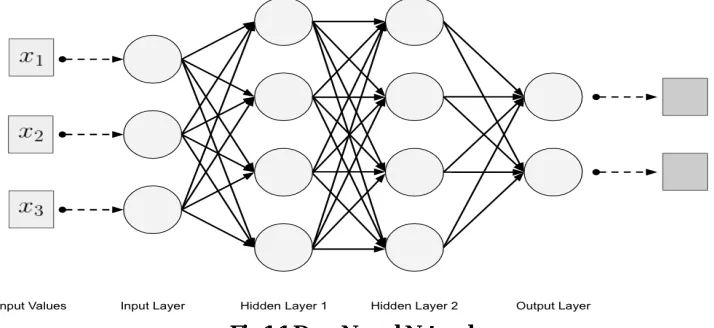
Deep Learning, as a branch of Machine Learning, utilizes calculations to process data and copy the thinking method, or to make deliberations. Deep Learning (DL) uses layers of calculations to process data, appreciate human discourse, and see objects. Information is experienced each layer, with the yield of the past layer offering commitment to the accompanying layer as appeared in fig1.1. The essential layer in a framework is known as the input layer, while the last is called a output layer. Each one of the layers between the two are called as hidden layers. Each layer is a direct, uniform computation containing one kind of activation function [1].

Deep learning includes a class of models which attempt to progressively learn deep highlights of info information with deep neural systems, regularly more profound than three layers. The system is first layer-wise introduced by means of unsupervised preparing and afterward tuned in an administered way. In this plan, abnormal state highlights can be gained from low-level ones, while the correct highlights can be figured for design arrangement at last. Deep models can possibly prompt continuously more theoretical and complex highlights at higher layers, and more dynamic highlights are for the most part invariant to most nearby changes of the info. As indicated by some recent papers [1], [2], deep models can give preferred estimate to nonlinear capacities over shallow models.

Typical deep neural network architectures include deep belief networks (DBNs) [3], deep Boltzmann machines (DBMs) [4], SAEs [5], and stacked denoising AEs (SDAEs) [6].

The layer-wise training models have a bunch of alternatives such as restricted Boltzmann machines (RBMs) [7], pooling units [8], convolutional neural networks (CNNs) [9], AEs, and denoising AEs (DAE) [5].

II. RELATEDWORK

Picture order was one of the main issues in the period of PC supported medicinal determinations frameworks. In its beginning times, the fundamental approach was to utilize handmade highlights, for example, Local Binary Pattern (LBP) [10][11] and Scale-Invariant Feature Transform (SIFT) [12] with multi-class order calculations, for example, Support Vector Machine (SVM) [13]. Be that as it may, carefully assembled highlights were tedious and requires master learning in picture preparing, human vision, and the specific space of the order issue. Here comes the requirement for programmed learning calculations that imitates human vision and requires less master information.

In the most recent 1950s, Hubel and Wiesel [14] thought of an extreme investigation that demonstrates the instrument in which human brains respond to various shapes and shades that are gotten by the human vision framework. That review demonstrates that the building square of the human recognition framework is made of what they have called a perceptron, which can be basically communicated scientifically as the summation of the weighted sources of info that will additionally deliver a positive or negative flag in view of the weighted total. What's more, a gathering of those perceptrons are then having their yield motions as contributions to another layer of perceptrons, et cetera. Yet, since that time, the execution of that strategy was not ready to demonstrate an incredible execution change in the order undertakings until 2012. Also, the principle purpose behind that is the way that such a design needs great computational power a long with a decent and sufficiently enormous dataset of very much marked pictures to be prepared on. The main restriction is getting dispensed with by the large scale manufacturing advancement we are as of now living in. While the second constraint is wiped out at present utilizing distinctive information increase systems that are appropriate for the given issue.

The outcomes Krizhevsky et al [15] have accomplished for the ImageNet characterization rivalry in 2012 were extraordinary.

With one thousand classes of in excess of a million picture, the issue is troublesome notwithstanding for a human master. The precision they have accomplished was 83% for the main 5 forecasts utilizing a profound Convolutional Neural Network with the greater part a million perceptron. They utilized two separate GPUs to prepare their system in around seven long stretches of preparing time. figure[1] demonstrates the design of their system that still moves junior specialists who are right now working in this field.

III.PROPOSEDALGORITHM

In this research, CNN parameters as described below are systematically varied and the classification accuracies are recorded.

Input image size

Number of neurons ( ), in the first convolutional layer Number of layers, M and N

In the proposed design, the CNN architecture stacks a few CONV - RELU layers (e.g. M number of layers), followed by pooling layers (optional). This pattern is repeated N times until the image has been merged spatially to a small size. At the end, there is a Fully-Connected (FC) layer to hold the output called as class score. Each neuron, of each layer computes following activation function.

f(x )=φ(wT x +b ) (1)

where x is the input to the neuron,w is a weight vector, b is a bias term and φ is a nonlinear function. Each neuron multiple inputs and produces a single output.

The convolutional layer is the main building block of a CNN; it consists of a set of learnable filters. Every filter is spatially small (spans along width and height), but extends through full depth of input volume. In forward pass, each filter slides across width and height of input volume and generated dot product between entries of the filter and input at the position, this generates a 2-D activation map which gives the responses of that filter at every spatial position. These 2-D activation maps are stacked along depth and output volume is produced. So, the output volume can be stated as a function of input volume.

IV.RESULTS

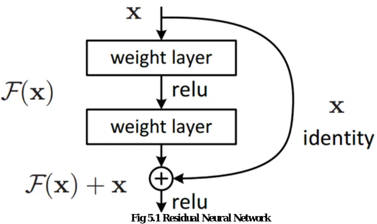
The main common trend in convolutional neural network models is their increasing depth. The increasing depth involves an increasing error rate, not due to overfitting but to the difficulties to train and optimize an extremely deep models. “Residual Learning” has been introduced to create a connection between the output of one or multiple convolutional layers and their original input with an identity mapping. In other words, the model is trying to learn a residual function which keeps most of the information and produces only slight changes. Consequently, patterns from the input image can be learned in deeper layers. Moreover, this method doesn’t add any additional parameter and doesn’t increase the computational complexity of the model. This model, dubbed “ResNet”, is composed of 152 convolutional layers with 3x3 filters using residual learning by block of two layers. Although it got a top-5 error rate of 4.49% over the 2012 ImageNet challenge (less than the Inception V3), the ResNet model has won the 2015 challenge with a top-5 error rate of 3.57%.

The principle normal pattern in convolutional neural system models is their expanding profundity. K. He et al. (2015) saw notwithstanding, that the expanding profundity includes an expanding mistake rate, not because of overfitting but rather to the challenges to prepare and advance a to a great degree profound models. "Remaining Learning" has been acquainted with make an association between the yield of one or different convolutional layers and their unique contribution with a character mapping. As it were, the model is attempting to take in a leftover capacity which keeps a large portion of the data and creates just slight changes. Therefore, designs from the information picture can be learned in more profound layers. In addition, this strategy doesn't include any extra parameter and doesn't expand the computational multifaceted nature of the model. This model, named "ResNet", is made out of 152 convolutional layers with 3x3 channels utilizing lingering learning by square of two layers. In spite of the fact that it got a best 5 blunder rate of 4.49% over the 2012 ImageNet challenge (not as much as the Inception V3), the ResNet show has won the 2015 test with a best 5 mistake rate of 3.57%.

Activation Description

Conv Convolution response images

ReLU Rectified Linear Units response images

Pool Max pooling response images

Incep Inception Module response images

Batch Batch Normalization response images

Fig 5.1 Residual Neural Network

Different Techniques have been produced to help neural systems when all is said in done and CNNs particularly. One of them is gotten Drop-Out [18], which empowers the system to have the capacity to sums up however much as could reasonably be expected to new test sets by dropping a portion of the neurons in a portion of the last completely associated layers. Drop-Out is a great procedure to abstain from overfitting issue amid preparing time. Another valuable system is channel based group standardization [19] after each convolutional layer. Batch normalization accelerates the preparation procedure by lessening the inside covariant move as expressed in their paper. That is essentially done by having each channel zero focused at each cycle of the preparation procedure. In addition, Data Augmentation additionally helps in preparing CNNs. It is vital on the grounds that it can expand the dataset estimate, which is useful for neural system preparing when all is said in done, while averting over-fitting the training set in the meantime [15].

V. CONCLUSIONANDFUTUREWORK

In DNCNN, traditional convolutional layers are replaced with normalization and convolutional layers to accelerate the training process and boost the performance. The numbers of layers and input window size have significant impact on accuracy for CIFAR-10 dataset. The highest classification accuracy of 81% was obtained with input image size 32×32×3, number of filters 28, filter size 5x5 and 13 layers, which is better than the best accuracy obtained by standard Alexnet classification accuracy of 77.75% on CIFAR-10 dataset. By increasing input image size, the classification accuracy increases to reach a maximum accuracy point and then it declines on further increase of input image size, so it can be considered as optimal input image size. Moreover, we also validate the importance and effectiveness of data augmentation for our DNCNN, especially when the training samples are insuffcient and imbalanced.

REFERENCES

[2] N. LeRoux and Y. Bengio, “Deep belief networks are compact universal approximators,” Neural Comput., vol. 22, no. 8, pp. 2192–2207, Aug. 2010.

[3] G. E. Hinton, S. Osindero, and Y. Teh, “A fast learning algorithm for deep belief nets,” Neural Comput., vol. 18, no. 7, pp. 1527–1554, Jul. 2006. [4] R. Salakhutdinov and G. E. Hinton, “Deep Boltzmann machines,” in Proc. Int. Conf. Artif. Intell. Statist., Clearwater Beach, FL, USA, 2009, pp. 448–455.

[5] Y. Bengio, P. Lamblin, D. Popovici, and H. Larochelle, “Greedy layer-wise training of deep networks,” in Proc. Neural Inf. Process. Syst., Cambridge, MA, USA, 2007, pp. 153–160.

[6] P. Vincent, H. Larochelle, I. Lajoie, Y. Bengio, and P. Manzagol, “Stacked denoising autoencoders,” J.Mach. Learn. Res., vol. 11, no. 12, pp. 3371–3408, Dec. 2010.

[7] G. E. Hinton, “Apractical guide to training restricted Boltzmann machines,” Dept. Comput. Sci., Univ. Toronto, Toronto, ON, Canada, Tech. Rep. UTML TR2010-003, 2010.

[8] Y. LeCun et al., “Backpropagation applied to handwritten zip code recognition,” Neural Comput., vol. 1, no. 4, pp. 541–551, Apr. 1989. [9] K. Fukushima, “Neocognitron: A self-organizing neural network model for a mechanism of pattern recognition unaffected by shift in position,” Biol. Cybern., vol. 36, no. 4, pp. 193–202, Apr. 1980.

[10] T. Ojala, M. Pietik¨ainen, and T. M¨aenp¨a¨a, “Gray scale and rotation invariant texture classification with local binary patterns,” in European Conference on Computer Vision. Springer, 2000, pp. 404–420.

[11] T. Ojala, M. Pietikainen, and T. Maenpaa, “Multiresolution gray-scale and rotation invariant texture classification with local binary patterns,” IEEE Transactions on pattern analysis and machine intelligence, vol. 24, no. 7, pp. 971–987, 2002.

[12] D. G. Lowe, “Object recognition from local scale-invariant features,” in Computer vision, 1999. The proceedings of the seventh IEEE international conference on, vol. 2. Ieee, 1999, pp. 1150–1157.

[13] C. Cortes and V. Vapnik, “Support vector machine,” Machine learning, vol. 20, no. 3, pp. 273–297, 1995.

[14] D. H. Hubel and T. N. Wiesel, “Receptive fields of single neurones in the cat’s striate cortex,” The Journal of physiology, vol. 148, no. 3, pp. 574–591, 1959.

[15] A. Krizhevsky, I. Sutskever, and G. E. Hinton, “Imagenet classification with deep convolutional neural networks,” in Advances in neural information processing systems, 2012, pp. 1097–1105.

[18] N. Srivastava, G. E. Hinton, A. Krizhevsky, I. Sutskever, and R. Salakhutdinov, “Dropout: a simple way to prevent neural networks from overfitting.” Journal of machine learning research, vol. 15, no. 1, pp. 1929–1958, 2014.