ABSTRACT
ZOU, XIAOCHENG. Enabling Efficient Scientific Analytics over Extreme-scale Adaptive Mesh Refinement Data through Effective In Situ Indexing. (Under the direction of Nagiza F. Samatova.)
One of the most significant advances for large-scale scientific simulations has been the ad-vent of Adaptive Mesh Refinement, or AMR. By dynamically adapting simulation resolution across space and time, AMR simulation codes can drastically improve efficiency of computa-tional resources while meeting or exceeding acceptable error levels for numerical convergence. Yet, this greatest strength of AMR—dynamic adaptivity—is also becoming its biggest weak-ness: the hierarchical, complex structure of AMR data renders existing indexing and query pro-cessing techniques ineffective, which greatly hinders data exploration and analytics on AMR data. Furthermore, the rising scale of AMR simulations, along with the growing strain on I/O resources, points toward a need forin situindexing to facilitate scientific analysis by reducing the time-to-analysis.
Among numerous scientific data explorations and analytics on AMR data,connected com-ponent detectionis a fundamental and important operation as many forms of analysis, such as isosurface, identification of level sets, and feature extraction, are often transformed into con-nected component detection tasks. However, detecting concon-nected components over AMR data is challenging because existing algorithms, primarily designed for detecting connected compo-nents on uniform grids, are not applicable to the intricate structure of AMR. Moreover, enabling such detection in the real-time requires a sustainable and scalable approach. To address this, we present the first parallel,in situconnected component detection methodology on structured AMR. Our key strategy is the incorporation of an multi-phase AMR-aware communication pat-tern that synchronizes connectivity information across the AMR hierarchy to detect the global connected components. In addition, we distill our methodology to a generic framework within the Chombo AMR infrastructure, making connected component detection services available for many existing applications. We demonstrate our method’s efficacy by showing its ability to detect ice calving events in real time within the real-world BISICLES ice sheet modeling code. Results show up to a 6.8x speedup of our algorithm over the existing specialized BISICLES algorithm. We also show scalability results for our method up to 4,096 cores using a parallel Chombo-based benchmark.
homo-geneous (with respect to same characteristic) regions for relatively simple analysis tasks. Many complex analytics (i.e., query-driven analysis, generally performed through SQL-like queries), however, are required to perform on varying input values in order to capture the cause and evo-lution of the regions and phenomena of interest. Not surprisingly, these complicated analytics would lead to intensive computation as operations of searching critical information of regions of interest over extreme-scale datasets need to be repeatedly performed for every new input value. Hence, we bring thefirstAMR-awarein situindexing and scalable querying methodol-ogy for complex scientific analytics on the AMR data. We first design a hybrid AMR-aware index structure, which consists of a spatial index component, organizing AMR boxes into cov-ering relations by a Directed Acyclic Graph (DAG), and a value index component, indexing data points within every AMR boxes by leveraging any existing value index technique, e.g., bitmap index, ALACRITY index, etc. We then present anin situ, query-optimized, AMR-aware indexing method that efficiently builds an AMR-specific index in a massively parallel manner. We last develop a parallel, AMR-index-aware, workload-balanced query processing method. We demonstrate the scalability of our in situ indexing using up to 16,384 cores, and that of our querying using up to 1,024 cores with the Chombo-IO benchmark. When compared to the non-AMR-aware indexing and querying, our AMR-aware indexing and querying demonstrate up to 12.4x and 500x, respectively.
Enabling Efficient Scientific Analytics over Extreme-scale Adaptive Mesh Refinement Data through Effective In Situ Indexing
by Xiaocheng Zou
A dissertation submitted to the Graduate Faculty of North Carolina State University
in partial fulfillment of the requirements for the Degree of
Doctor of Philosophy
Computer Science
Raleigh, North Carolina
2016
APPROVED BY:
Kemafor Anyanwu Ogan Rada Y. Chirkova
Ranga Vatsavai Nagiza F. Samatova
DEDICATION
BIOGRAPHY
ACKNOWLEDGEMENTS
First and foremost, I am eternally grateful to my advisor, Dr. Nagiza Samatova, for her constant guidance and inspiration throughout the entirety of my Ph.D. study. It was her continuous insight and guidance enlightens on my research path, especially when I need them most as I was a new PhD student. It was her determination of pursuing high goals keeps motivating me to improve my work quality. I am truly blessed to have her as my advisor. Without her support, I could not have reached this point.
Several other faculty in our Computer Science department at NC State University have had marked impact on my PhD study. I am very thankful to my committee members, Dr. Rada Chirkova, Dr. Kemafor Ogan, and Dr. Raju Vatsavai, for taking their valuable time to serve on my thesis committee, and for offering their critical insight in this thesis. I am grateful to Dr. Douglas Reeves for admitting me into the Ph.D. program with funding. I would also like thank Dr. David Thuente and Dr. Matthias Stallmann, from whose courses I had the privilege to learn critical thinking, mathematical and algorithmic reasoning skills.
Over the period of this dissertation I have had the pleasure of collaborating with several experts at various national laboratories in the field of High Performance Computing: John (Kesheng) Wu, Suren Byna, Dan Martin, and Hans Johansen from Lawrence Berkeley Na-tional Laboratory (LBNL), Scott Klasky, Norbert Podhorszki and Qing Liu from Oak Ridge National Laboratory and Rob Ross and Dries Kimpe from Argonne National Laboratory. I am thankful to them for providing me access to leadership class computing resources and the nec-essary software infrastructure for me to work with. The summer I spent at LBNL, working with Jonn Wu, Suren Byna, and Dan Martin with whom I had numerous useful discussion, was particularly fruitful. I am in particularly grateful to John Wu and Suren Byna, who made valu-able suggestions that had significant performance improvement on the parallel, AMR-aware connecting component labeling algorithm. I am also thankful to Dan Martin who patiently explained to me the Chombo library and the BISICLES application, which are two fundamen-tal components in my implementation. Additionally, the resultant work has became the first chapter of this thesis and has laid the foundation of this entire thesis.
especially thankful to David (Drew) Boyuka, who is a contemporary of mine in the group, and has been a long-time collaborator, and is good friend to me. Houjun Tang deserves a spe-cial mention for being a good collaborator and a good friend to me as well. In addition, I am grateful to many students, including but not limited to, Dhara Desai, Wenzhao Zhang, Steven Harenburg, Stephen Ranshous, Eric R. Schendel, Gonzalo Bello Lander, and Kushal Bansal for their assistance during my PhD study.
I would also like to thank those who mentored me before coming to NC State university. Foremost among these is Dr. Jing Deng, a professor of computer science at the University of North Carolina at Greensboro (UNCG). He supported me as a Graduate Research Assistant in the computer science department at UNCG. Without his support, I could not have achieved my dream of studying computer science in the U.S. In addition, Dr. Deng taught me research skills and inspired me to do high quality research. Furthermore, I would like to thank Dr. Shan Suthaharan, Dr. Fereidoon (Fred) Sadri, Dr. Nancy Green and Dr. Francine Blanchet-Sadri, for teaching several graduate classes, which prepared me for my PhD program.
Most importantly, I am thankful to my family for their unconditional love and support. My father Zhenxin Zou, and mother Zhenqin Lu, have been a blessing in my life in more ways than I can count. They came to the USA for one year to look after my son Jason, which was a tremendous support for allowing me time to work on this thesis. I am so very grateful to have an angel baby Jason, who brings us a lot of joy and happiness. Last but not least, I am deeply grateful to my wife Jinni Su’s support and encouragement throughout my graduate study. She has always been there for me, wishing me to success.
TABLE OF CONTENTS
LIST OF TABLES . . . viii
LIST OF FIGURES . . . ix
Chapter 1 Introduction . . . 1
1.1 ParallelIn SituDetection of Connected Components in Adaptive Mesh Refine-ment Data . . . 2
1.1.1 Problems and Challenges . . . 2
1.1.2 Approach and Results . . . 3
1.2 Effective In Situ Indexing over Extreme-scale Adaptive Mesh Refinement Data 4 1.2.1 Problems and Challenges . . . 4
1.2.2 Approach and Results . . . 5
1.3 Fast Set Intersection through Run-time Bitmap Construction over PForDelta-compressed Indexes . . . 6
1.3.1 Problems and Challenges . . . 6
1.3.2 Approach and Results . . . 7
Chapter 2 ParallelIn SituDetection of Connected Components in Adaptive Mesh Refinement Data. . . 8
2.1 Introduction . . . 8
2.2 Problem Statement . . . 10
2.3 Method . . . 14
2.3.1 Connected Component Labeling for AMR Data . . . 14
2.3.2 In SituAMR-aware Connected Component Labeling . . . 17
2.4 Experimental Evaluation . . . 22
2.4.1 Experimental Setup . . . 23
2.4.2 BISICLES – Real-Time Ice Calving Detection Use Case . . . 23
2.4.3 Packed Channel – Large-scale Chombo Benchmark . . . 26
2.5 Related Work . . . 29
2.6 Conclusion . . . 30
Chapter 3 AMR-aware In Situ Indexing and Scalable Querying . . . 31
3.1 Introduction . . . 31
3.2 Problem Statement . . . 33
3.3 Method . . . 36
3.3.1 A Hybrid, AMR-aware Index . . . 36
3.3.2 In Situ, AMR-aware Indexing . . . 37
3.3.3 Scalable AMR-index-aware Querying . . . 41
3.4.1 Experimental Setup . . . 43
3.4.2 AMR-aware Indexing Evaluation . . . 43
3.4.3 AMR-index-aware Querying Evaluation . . . 45
3.5 Related Work . . . 47
3.6 Conclusion . . . 47
Chapter 4 Fast Set Intersection through Run-time Bitmap Construction over PForDelta-compressed Indexes . . . 55
4.1 Introduction . . . 55
4.2 Related Work and Background . . . 56
4.2.1 Set Intersection . . . 56
4.2.2 PForDelta-compressed indexes . . . 57
4.3 Method . . . 58
4.3.1 The Role of Set Intersection in Conjunctive Query Processing . . . 58
4.3.2 BitRun: Incorporating Run-length Encoding into PForDelta . . . 60
4.3.3 BitExp: Expanding the PForDelta Encoding Bit-Width . . . 61
4.3.4 BitRun-BitExp: Handling Set Intersections across Heterogeneous Datasets 63 4.4 Results . . . 63
4.4.1 Experimental Setup . . . 63
4.4.2 Comparison with WAH bitmap indexes . . . 65
4.4.3 Performance Breakdown of PForDelta-compressed Index Approaches . 65 4.5 Conclusion . . . 67
Chapter 5 Conclusion . . . 70
5.1 Conclusion . . . 70
5.2 Future Work . . . 70
5.2.1 Data storage to facilitate heterogeneous data accesses induced by query-driven analytics . . . 71
5.2.2 In situ interactive query processing . . . 72
LIST OF TABLES
LIST OF FIGURES
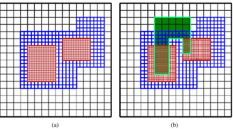
Figure 2.1 Subfigure (a) shows an AMR mesh with three levels: the black mesh is the coarsest mesh (level 0), the blue mesh is a finer mesh (level 1), and the red mesh is the finest (level 2). The refinement ratio equals 2.Subfigure (b) shows a connected component that has been detected, spanning all three AMR levels. . . 10 Figure 2.2 Subfigure (a) shows a two-dimensional example of an AMR hierarchy
with refinement ratio 2 and two levels. It also indicates pairs of adjoin-ing cells on the same level and on different levels, as well as a pair of overlapping cells. Subfigure (b) illustrates the coarsening and refine-ment operators at refinerefine-ment ratio 2, as defined in Definition 1 of the Problem Statement. . . 11 Figure 2.3 An example showing the communication pattern in our parallel,in situ
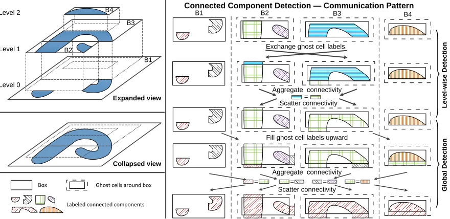
connected component detection over four AMR boxes. On the left, the component being detected is illustrated with both expanded and col-lapsed views. . . 15 Figure 2.4 An example showing provisional labels are produced by the first pass
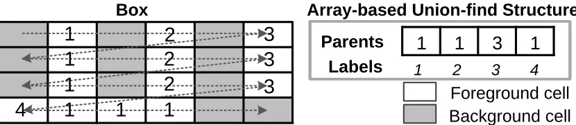
of the SAUF algorithm on a 4×6 box (left), along with the correspond-ing union-find structure UF (right). The dash arrow indicates the scan traversal order (raster order). The UF structure indicates that labels 1, 2, and 4 are equivalent, and thus collectively form a component (label 3 represents a second component). . . 16 Figure 2.5 An example of an ice calving event on the Pine Island Glacier ice shelf
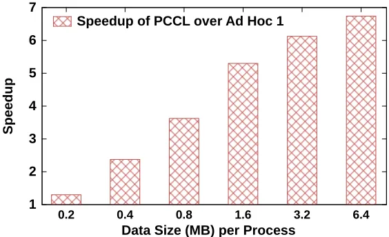
during the simulation run is shown. The glacier is shown before (sub-figure (a)) and after (sub(sub-figure (b)) the calving event occurs, wherein a rectangular region of ice (approximately 30km×26km in real size) detaches from the main shelf and becomes an isolated floating iceberg. Subfigure (c) shows an ice thickness mapping over the whole of the Antarctica glacier, surrounded by ocean (dark blue). . . 24 Figure 2.6 Speedup ofPCCLoverAd Hoc 1for real-time ice calving event
detec-tion in BISICLES. . . 25 Figure 2.7 Speedup ofPCCLoverAd Hoc 1in a BISICLES run where no calving
occurs for many consecutive timesteps. Greater speedups are observed at larger per-process data sizes, as before. This speedup is consistent as more no-calving timesteps transpire. . . 26 Figure 2.8 A depiction of a 2D packed channel dataset. The circular regions in the
Figure 2.9 A timing breakdown comparison betweenPCCL andAd Hoc 2for an AMR dataset with 800 million total cells when run on Edison.PCCL
achieves a consistent speedup overAd Hoc 2, up to 1.4x. . . 28
Figure 3.1 Subfigure (a) shows an example of a 3-level AMR mesh with refine-ment ratio 2: from the coarsest to the finest level. The black mesh is the coarsest mesh (level 0), the orange mesh is a finer mesh (level 1), and the green mesh is the finest (level 2). Subfigure (b) illustrates a 2-level AMR hierarchy, with three box types: 1) B0,2,B1,0, and B1,1 are
uncovered; 2) B0,0 andB0,3 are partially covered; and 3) B0,1 is fully covered. . . 33 Figure 3.2 Subfigure (a) shows a 3-level AMR hierarchy with boxes highlighted on
each level. Subfigure (b) illustrates an AMR-aware hybrid index built from the left AMR hierarchy. . . 37 Figure 3.3 Weak scaling performance of the AMR-aware indexing with ≈40MB
and 35MB data size per-process (total 650GB and 570GB) for 2D and 3D runs, respectively. . . 49 Figure 3.4 Strong scaling performance of the AMR-aware indexing with total≈
325GB and 285GB data size for 2D and 3D runs, respectively. . . 50 Figure 3.5 The overhead of the AMR-aware,in situindexing in a BISICLES run
for consecutive 90 time-steps. Subfigure (a) and (b) show percentage of indexing (CPU) and end-to-end (CPU + I/O) time added on original BISICLES time, respectively. . . 51 Figure 3.6 Performance (subfigure (a)) and storage increase (subfigure (b))
com-parison between our AMR-aware in situ indexing and a non-AMR-awarein situindexing,flattening. . . 52 Figure 3.7 Scalable query performance with a fixed query selectivity of 1%
(sub-figure 3.7 (a)) and a fixed process number of 256 (sub(sub-figure 3.7 (b)) at four index aggregation levels. . . 53 Figure 3.8 Speedup of our AMR-aware querying over the scan approach for 2D
and 3D AMR. . . 54
Figure 4.1 Overview of our set intersection approach using PForDelta-compressed indexes fits into conjunctive query processing. . . 59 Figure 4.2 An example of how PForDelta encodes a chunk of mostly-sequential
Figure 4.3 PForDelta decoding time when varying|E|while keepingbfixed (left), and when varyingb while keeping|E|fixed (right). Reported timings are for decoding 1000 PForDelta chunks. Trends seen are representative of experiments with otherband|E|parameters. . . 62 Figure 4.4 Comparison of query response times betweenBRBEandWAH. Results
for two-constraint queries are similar, but are omitted for space consid-erations. . . 66 Figure 4.5 Comparison of query response times amongBitRun,BitExp, andBRBE,
Chapter 1
Introduction
Adaptive Mesh Refinement (AMR) [3, 5, 9–11, 15, 61] for large-scale scientific simulations has enabled to achieve substantial savings in memory, computation, and storage resources while maintaining or even increasing simulation accuracy [24, 49]. With AMR, across dif-ferent time steps, simulation codes dynamically discretize the continuous domain of interest into an adaptive grid of individual elements while balancing between the size of the spatial res-olution and the acceptable error. Applications that have successfully applied the AMR model include astrophysics simulations (Enzo [27, 66] for cosmological structure formation, GenA-SiS [14, 18, 32, 33] focusing on neutron star mergers and core-collapse supernovae, and oth-ers [34, 51, 52, 82]), nuclear reactions (e.g., UNIC [67] for neutronics and thermal hydraulics), and chemistry (e.g., MADNESS [41] for quantum chemistry in multiwavelet bases).
the data exploration and analysis by quickly narrowing down the subset data of interest from extreme-scale datasets.
Unfortunately, existing indexing and query approaches [45,84] are not designed for AMR’s complex spatio-temporal structural adaptivity, and fall short in capabilities needed by complex scientific discovery. In particular, current indexing methods are largely designed for process-ing homogeneous data records, such as rows of a data table or tuples of a relation, and have difficulty in handling the heterogeneous, hierarchical, and spatio-temporal evolution aspects of AMR data. Furthermore, as factors consisting of AMR data (i.e., hierarchical structure, logi-cally rectangular boxes, and data points in boxes) typilogi-cally exhibit different characteristics, an effective indexing should be holistic so that it can capture the essence of the AMR data.
Therefore, we present an AMR-aware analysis framework to enable the efficient scientific exploration and analysis on AMR data. We first present a parallel, scalable in situ approach which detects connected components that distributed over AMR data to address the efficiency of the core operation in various AMR analyses. Based on this, we further present a hybrid AMR-aware indexing technique that facilitates performing a serial of connected component detection operations with a varying threshold value over extreme-scale data for complex anal-ysis tasks.We finally present anon-the-flyindex conversion approach to process heterogeneous indexes in the hybrid AMR-aware indexing in support of efficient query processing. Next, we briefly summarize the motivations and contributions of our work.
1.1
Parallel
In Situ
Detection of Connected Components in
Adaptive Mesh Refinement Data
1.1.1
Problems and Challenges
Developing a connected component detection algorithm for AMR data is not a trivial task, however. Existing detection algorithms, generally categorized as one-pass [20, 43, 83], two-pass [37,62,65,89], and multi-two-pass [76], are designed for single-level, uniform meshes, and thus are not applicable to data that span multiple levels in an adaptive refinement mesh. Attempting to “flatten” an AMR hierarchy to a uniform mesh (refining all mesh levels up to the finest resolution) in order to apply existing algorithms has its own problems: such an operation results in an explosive increase in memory usage, which is untenable for extreme-scale datasets, and in any case defeats one primary goal of using AMR in the first place.
Beyond the general problem of AMR-aware connected component detection, achieving vi-able in situdetection is a challenge. Anyin situ processing must have minimal performance impact on the overall simulation. Yet, parallel connected component detection is inherently characterized as communication-intensive, and the non-uniform, distributed nature of AMR data exacerbates this state of affairs. Specifically, the distribution of mesh data across pro-cesses in AMR simulations is typically bothnon-regular anddynamic over time, making syn-chronization of connectivity information inherently more difficult than with the regular domain decompositions applied to uniform meshes.
1.1.2
Approach and Results
To the best of our knowledge, AMR connected component detection has not been explored in literature. Therefore, we first formally define the general problem of connected component detection that is specifically tailored for AMR data. By adapting the traditional definitions of mesh, adjacency, and connectivity, we clearly articulate the problem to be solved, which we expect will benefit future work in this area. We then describe our solution to the AMR connected component detection problem.
In addition, we distill our parallel in situapproach to a general-purpose AMR-aware con-nected component detection framework in the Chombo infrastructure [1], a popular block-structured AMR framework used by many scientific applications [28, 69, 80]. In this way, we demonstrate the general applicability of our work to scientific codes.
The work is published in the 15th IEEE/ACM International Symposium on Cluster, Cloud and Grid Computing (CCGrid’15) [95].
1.2
Effective In Situ Indexing over Extreme-scale Adaptive
Mesh Refinement Data
1.2.1
Problems and Challenges
Our previous approach addresses the efficiency of a fundamental operation, connected compo-nents detection on AMR data, in various scientific explorations. The detection approach begins with a fixed threshold value that is used to divide the whole mesh structure into foreground and background parts.
However, complex analysis tasks, i.e., query-driven analysis (generally performed through SQL-like queries), are required to perform on varying input values (with regard to every iter-ation) in order to capture the cause and evolution of the regions and phenomena of interest. For example, in climate science, an atmospheric river can be detected using a query with both a spatial selection (the West Coast of North America) and value constraint (Integrated Water Vapor > 2cm) [17]. In another example, fluid velocity change in turbulent flow simulations can be tracked by a query such as “-72.28 cm/sec ≤velocity ≤96.77 cm/sec” at the region around the corner of a drill pipe [81].
A straight forward approach for supporting query-driven analysis on AMR data is known as“flattening.” In this approach, all mesh levels are refined to the finest resolution to form a uniform grid, allowing the direct application of non-AMR indexing and query methods with-out special modification. For example, the QDV system [36] supports the SQL-like queries on the AMR data by performing bin-hash indexing on a single-level, “synchronized” mesh data flattened from multiple AMR datasets. However, we argue that the “flattening” operation causes an explosive increase in the storage and memory requirements. For example, flattening an AMR grid with 5 levels of refinement to the finest level could increase its storage footprint by up to 1000x. This is untenable for extreme-scale datasets, and in any case defeats one pri-mary purpose of using AMR in the first place. Therefore, there is a need to enable querying capabilities directly on AMR data by embracing the AMR structure.
such as Fastbit [84] and ALACRITY [46], are prominently designed for capturing value char-acteristics on a single, uniform mesh data; Instead, we need a new indexing capable of handling the hierarchical, non-uniform AMR data that characterizes both value and space aspects at the same time. Furthermore, as demonstrated in the early work [12, 48, 53], an effective and sus-tainable indexing technique towards the future extreme-scale computation needs to operate in the context ofin situwhere the indexing runs concurrently with the simulation run. Hence, we advocate for anin situ, scalable, and AMR-aware indexing.
While appealing, this shift in indexing technique presents unprecedented challenges. As a generalin situalgorithm, it inevitably faces the challenge of minimizing its performance dis-turbance to the simulation run [48,53,95]. Moreover, as a specific AMR-awarein situindexing, it faces further challenges: the scattered AMR hierarchy across processes, typically character-izing both non-regular and dynamic over time, makes building an index more difficult than uniform meshes distributed by regular domain decompositions.
Subsequently, this necessary shift in indexing paradigm raises corresponding challenges on the query side. That is, developing an AMR-aware querying (assuming indexes have been built) needs an efficient, parallel query processing strategy in order to support large-scale scientific discoveries. As the query processing is “sandwiched” by the end-users and the indexes, an effi-cient, parallel query processing faces the challenge from the combination of the unpredictable user-invoked queries and complicate AMR indexes. Specifically, the core challenge centers around the difficulty of achieving balanced querying workload in the parallel context as result of: 1) the irregular index read access patterns invoked by unpredictable queries [71, 72]; and 2) unbalanced AMR index sizes across levels.
1.2.2
Approach and Results
To address all these challenges, we propose thefirstAMR-awarein situindexing and scalable querying methodology for scientific exploration and analysis on the AMR data. Our contribu-tions are as follows:
• Formally define the general problem of query-driven analysis for AMR data. This for-mal definition paves the way for our systematic study of AMR indexing and querying problem.
• Develop a parallel,AMR-index-aware, workload-balancedquery processing method.
• Integrate both methods within the Chombo AMR infrastructure [2], this way we make our AMR-specific analysis services available for many existing Chombo-based applica-tions.
We demonstrate the scalability of ourin situindexing using up to 16,384 cores, and that of our querying using up to 1,024 cores with the Chombo-IO benchmark [19]. When compared to the non-AMR-aware indexing and querying, our AMR-aware indexing and querying demon-strate up to 12.4x and 500x, respectively. We also measurethe overhead of ourin situindexing within the BISICLES [28] ice sheet modeling code, demonstrating its impact on the simulation run to be negligible.
This work has received the Best Paper Award at 24th High Performance Computing Sym-posium (HPC 2016) and the second Best Paper Award at Spring Simulation Multi-Conference 2016 (SpringSim’16) [93].
1.3
Fast Set Intersection through Run-time Bitmap
Construc-tion over PForDelta-compressed Indexes
1.3.1
Problems and Challenges
SQL-like queries are often used by scientists to narrow down the region of interest or discover important scientific phenomena in an exploratory manner. For example, scientists may use the “density> 1.5 AND 100<time step < 95” query to analyze how the spatial distribution of gas densities varies in the temporal dimension within shock-wave simulations. Performance of the query processing that answers queries is often improved with the help of indexes.
index decompression followed by multiple expensive list merge and intersection operations. Abandoning any index may not be desirable in many cases, since each index type has its own advantages and thus is a valuable asset for data-intensive analysis tasks.part
1.3.2
Approach and Results
We propose anon-the-flyindex conversion approach that can effectively bridge the gap between storage-efficient CIIs, and multivariate query-optimized bitmap indexes. By building bitmaps in-tandem with CII decompression, the highly optimized bitwise instructions supported by modern high performance computing architectures can be utilized to perform fast bit-based query processing without paying the storage cost of a bitmap index. Ensuring this efficient bitmap conversion step is the central issue.
To this end, we contribute two key enhancements to PForDelta, BitRun and BitExp, that greatly improve bitmap conversion through bulk bit-setting and a more streamlined PForDelta decoding process, respectively. BitRun incorporate a run-length encoding in PFor-Delta by tak-ing advantage of the consecutiveness property of encodtak-ing data. This incorporated encodtak-ing schema describes the number of consecutive bits to be set and the number of bits to be skipped in bitmap. In such a way, it enables to set a sequence of bits in the bitmap concurrently, rather than one bit at a time during the bitmap construction. Whereas, BitExp breaks the convention that a PFor-Delta chunk typically achieves the greatest compression ratio, but not the highest decoding throughput. And it uses a larger encoding bit (expanding) which enables the PFor-Delta chunk to have a maximum decoding throughput. To avoid taxing a large increase storage overhead, the chunks to be “expanded” is carefully selected, with the goal of trading a small amount of storage for a large gain in throughput. Our experimental results show that our in-tegrated PForDelta-bitmap approach speeds up conjunctive queries by up to 7.7x versus the state-of-the-art pure bitmap-based method, while using 15-60% less index storage space in most cases.
Chapter 2
Parallel
In Situ
Detection of Connected
Components in Adaptive Mesh
Refinement Data
2.1
Introduction
One of the most significant advances for large-scale scientific simulations has been the advent of Adaptive Mesh Refinement, or AMR [9–11]. By dynamically refining simulation resolution across space and time, AMR simulation codes can drastically improve efficiency of computa-tional resources while meeting or exceeding acceptable error levels for numerical convergence. The result of this refinement is a hierarchical, multi-level, and multi-resolution mesh (Fig. 2.1(a)), which gives rise to many opportunities and challenges in data analytics and visualiza-tion due to the intricate mesh structure.
As simulations transition to AMR, existing analysis and support algorithms must become AMR-aware to match. Connected component detection is one such algorithm, and is impor-tant to many scientific applications in bothin situandpost-processingcontexts. For example, the BISICLES AMR ice sheet modeling code [28] relies on the correctness-critical task of real-time isolated iceberg detection, which can be solved with efficientin situconnected com-ponent detection. Likewise, in the context of post-analysis, operations such as isosurfacing, identification of regions of interest, and hot spot isolation are often transformed into connected component detection tasks.
a trivial task, however. Existing detection algorithms, generally categorized as one-pass [20, 43, 83], two-pass [37, 62, 65, 89], and multi-pass [76], are designed for single-level, uniform meshes, and thus are not applicable to data that span multiple levels in an adaptive refinement mesh. Attempting to “flatten” an AMR hierarchy to a uniform mesh (refining all mesh levels up to the finest resolution) in order to apply existing algorithms has its own problems: such an operation results in an explosive increase in memory usage, which is untenable for extreme-scale datasets, and in any case defeats one primary goal of using AMR in the first place.
To the best of our knowledge, AMR connected component detection has not been explored in literature. Therefore, in this paper, we formally define the general problem of connected component detection that is specifically tailored for AMR data (Section 2.2). By adapting the traditional definitions of mesh, adjacency, and connectivity, we clearly articulate the problem to be solved, which we expect will benefit future work in this area. We then describe our solution to the AMR connected component detection problem in Section 2.3.1.
Beyond the general problem of AMR-aware connected component detection, achieving vi-able in situdetection is a challenge. Anyin situ processing must have minimal performance impact on the overall simulation. Yet, parallel connected component detection is inherently characterized as communication-intensive, and the non-uniform, distributed nature of AMR data exacerbates this state of affairs. Specifically, the distribution of mesh data across pro-cesses in AMR simulations is typically bothnon-regular anddynamic over time, making syn-chronization of connectivity information inherently more difficult than with the regular domain decompositions applied to uniform meshes.
To address this challenge, we present the first connected component detection methodology for structured AMR data that is applicable in a distributed,in situcontext (Section 2.3.2). Our key strategy is to use a parallel, in situ, AMR-aware communication method to synchronize component connectivity across the AMR structure distributed over many processes. By using a hierarchical process grouping conforming to the AMR refinement level structure, we are able to compute global connectivity over arbitrary distributions of AMR data without expensive all-to-all communication.
In addition, we distill our parallel in situapproach to a general-purpose AMR-aware con-nected component detection framework in the Chombo infrastructure [1], a popular block-structured AMR framework used by many scientific applications [28, 69, 80]. In this way, we demonstrate the general applicability of our work to scientific codes (Section 2.4).
(a) (b)
Figure 2.1: Subfigure (a)shows an AMR mesh with three levels: the black mesh is the coarsest mesh (level 0), the blue mesh is a finer mesh (level 1), and the red mesh is the finest (level 2). The refinement ratio equals 2. Subfigure (b)shows a connected component that has been detected, spanning all three AMR levels.
when applied to two simulation use cases. We use our framework to provide real-time ice calving detection for BISICLES, a large-scale AMR code, demonstrating viability for in situ
use (Section 2.1). Additionally, we apply our algorithm to the established “Packed Channel” benchmark [64, 79], for which our algorithm exhibits scalability up to 4,096 cores (Section 2.4.3).
2.2
Problem Statement
The ideal that most scientific simulations approximate is to evolve dependent variables (or
Level X
Y
(0,<1,0>)
(0,<1,0>) (1,<7,4>)(1,<7,4>) (1,<8,4>)(1,<8,4>)
(1,<3,2>) (1,<3,2>) (0,<1,1>) (0,<1,1>)
Overlap
(1,<2,3>) (1,<2,3>)
Adjoining Adjoining
(a)
X
Y
Level L
Level L+1
(6, 4) (7, 4)
(7, 5)
(6, 5)
(3, 2)
C (i, r=2)
R (i, r=2)
(b)
Figure 2.2: Subfigure (a) shows a two-dimensional example of an AMR hierarchy with re-finement ratio 2 and two levels. It also indicates pairs of adjoining cells on the same level and on different levels, as well as a pair of overlapping cells. Subfigure (b) illustrates the coarsen-ing and refinement operators at refinement ratio 2, as defined in Definition 1 of the Problem Statement.
simulation.
Of course, using a continuous domain is not possible with a finite computer, and so simula-tions necessarily operate on discretized domains. Although uniform meshes have traditionally been used for this purpose, Adaptive Mesh Refinement (AMR) has proven to be a memory- and computation- efficient alternative. AMR assigns different levels of resolution across the sim-ulation domain, delivering enough precision in highly-dynamic areas to achieve convergence, while also not over-provisioning more static regions.
This paper presents the first general-purpose method for connected component detection
clarify, we present a formal definition of connected component detection on AMR data. Then, we restate the problem using this formal language.
First, we define thecoarseningandrefinementoperators, which will be helpful later1: Definition 1:Thecoarsening operator C:ZD→ZDis defined asC(i,r) = (bi0
rc,b i1
rc, . . . ,
biD−1
r c), wherer∈Z
+is a givenrefinement ratio. Correspondingly, we define the opposite
re-finement operator R:ZD→P ZD
asR(i,r) ={i0∈ZD|C(i0,r) =i}. Equivalently,R(i,r) = ∏Dj=−01{rij,rij+1, . . . ,rij+r−1}, where∏is the N-ary Cartesian product. These operators can be naturally extended to operate on sets of vectors.
Next, we define the components of an AMR structure.
Definition 2: An AMR structure Ω with N ∈Z+ levels, domain bound u∈(Z+)D, and refinement ratior∈Z+consists of a list ofAMR levels
Ω0, . . . ,ΩN−1. For the first level,Ω0=
{i∈ZD|0≤i<u} with 0 denoting the zero vector and with < (≤) denoting the pairwise comparison of the components of two vectors. For subsequent levels,Ωl+1⊂R(Ωl,r). Finally, everyΩlcan be decomposed into a disjoint union ofmlrectangularboxes Bl,k⊂ZD such that Ωl=∪mk=l0Bl,kandBl,x∩Bl,y= /0 whenx6=y.
In other words, an AMR structure is a hierarchy of meshes, with the coarsest (lowest) level covering the whole computational domain, and successively finer (higher) levels covering portions of the next-coarser level. All mesh cells on a given level have the same spacing, with the grid spacing at each finer level reduced by a given refinement ratio relative to the next-coarser level. Additionally, in the specific case of block-structured AMR considered in this paper, each level’s mesh can always be decomposed in a set of non-overlapping rectangular regions calledboxes. Figure 3.1 sums up this definition with an example of a block-structured AMR hierarchy.
Definition 3:Acellat levellof AMR structureΩis defined as a pairc= (l,i)withi∈Ωl. The set of all cells in an AMR structureΩis denoted byσ(Ω) =
N−1 S l=0
(l,i)|i∈Ωl. Now, we define some properties of AMR cells.
Definition 4:Given two cellsc1= (l1,i1),c2= (l2,i2)in AMR structureΩ, we define the
1Definitions 1 and 2 are adapted from the Chombo framework design document [1]. For brevity, we have
adjoining predicate A:σ(Ω)×σ(Ω)→ {true,f alse}as
A(c1,c2) =
i1−i2∈E ifl1=l2
∃j∈R i2,rl1−l2
A((l1,i1),(l1,j)) ifl1>l2
A(c2,c1) else
withE={e0,−e0, . . . ,eD−1,−eD−1}the set of unit vectors aligned with a coordinate axis (such as(1,0,0),(−1,0,0),(0,1,0)). Cellsc1andc2are said to beadjoiningiffA(c1,c2).
Informally, two adjoining cells would be touching if the AMR hierarchy were “collapsed” or “flattened”.
Definition 5:Given two cellsc1= (l1,i1),c2= (l2,i2)in AMR structureΩ, we define the
overlap predicate B:σ(Ω)×σ(Ω)→ {true,f alse}as
B(c1,c2) =
i1=i2 ifl1=l2 i1∈R i2,rl1−l2
ifl1>l2
B(c2,c1) else
Cellsc1andc2are said tooverlapiffB(c1,c2).
Definition 6:Given an AMR structureΩ, acell-classifying predicateψ:σ(Ω)→ {true,f alse} classifies each cell as either aforeground(true) orbackground(f alse) cell. When ψ is under-stood by context, the set of foreground and background cells ofΩunderψ are denoted asΩFG andΩBG, respectively.
Note, ψ is typically is based on one or moredependent variablesdefined over the cells in Ω. Going back to our earlier example, BISICLES might choose ψ as a threshold on the ice thickness variable, thus identifying icebergs (foreground cells) disconnected from the main ice sheet by regions of thin or no ice (background cells).
Finally, we bring together previous concepts to define “connectedness” and “connected components”.
Definition 7: Given an AMR structure Ωwith cell-classifying predicate ψ defining fore-ground cellsΩFG, we define theadjacency relation∆on the foreground cells as∆={(c1,c2)∈
ΩFG×ΩFG|A(c1,c2)∧ ¬B(c1,c2)}.
Definition 8:Given the adjacency relation∆, we define theconnectivity relation∆+ as the
connected componentsP={ρ1, . . . ,ρ|P|}withρx∩ρy= /0↔x6=yandΩFG=∪ρ∈Pρ. We say two cellsc1,c2∈ΩFGareconnectediff(c1,c2)∈∆+.
That is, two foreground cells are connected if there exist zero or more other foreground cells that form a path of adjacent pairs (under adjacency relation ∆) between them. The resultant set of connected components P is a set of “regions” of cells, within which any two cells are connected.
We can now rephrase the problem statement more formerly:
Definition 9: Given an adaptive refinement mesh Ω and a cell-classifying predicate ψ, detect the set of connected components P of foreground cells ΩFG under the connectivity relation∆+
Beyond this basic definition, in order to feasibly runin situwith real-world simulations, any connected component detection method must meet two additional constraints. First, in order to operatein parallel,Ωmust be assumed to be distributed across multiple parallel processes. Second, when running in situ (that is, concurrent with a simulation), the solution must have limited runtime disturbance to the simulation (i.e., computation and communication overhead).
2.3
Method
Returning to the contributions for this paper, we propose a methodology that achieves two key goals, covered individually in the following subsections. First, we show how to solve the connected components detection problem for AMR data (as defined in the previous section); our key insights that make this possible are discussed in Section 2.3.1. Second, we show how to extend these principles to a parallel, in situ context, focusing on minimizing communica-tion and maximizing parallelism by using an AMR-aware communicacommunica-tion pattern, discussed in Section 2.3.2.
2.3.1
Connected Component Labeling for AMR Data
=
Aggregate connectivity Scatter connectivity Exchange ghost cell labels
Fill ghost cell labels upward
= Aggregate connectivity
Scatter connectivity Collapsed view = = = B4 B3 B2 B1 Expanded view
Connected Component Detection — Communication Pattern
B1 B2 B3 B4
Level 2
Level 1
Level 0
Box Ghost cells around box
Labeled connected components
L e v e l-w is e D e te c ti o n G lo b a l D e te c ti o n
Figure 2.3: An example showing the communication pattern in our parallel,in situconnected component detection over four AMR boxes. On the left, the component being detected is illus-trated with both expanded and collapsed views.
would produce correct results for a given traversal order.
Our key insight is to depart from scanning the AMR hierarchy as a single, indivisible mesh. Instead, we embrace the AMR structure by detecting components within each AMR box sep-arately, followed by joining these components in a global context. This has the advantage of a regular access pattern admitted by the individual uniform-mesh boxes.
This strategy is captured in Algorithm 1, which can be broken down into two phases.Phase I(lines 1 to 6) detects connected components within each level. Following this,Phase II(lines 7 to 10) then joins these intra-level components across levels, forming finalized global compo-nents.
As a preliminary detail, we briefly review the SAUF [89] algorithm, as we utilize this al-gorithm in some parts of our AMR detection solution. SAUF is a two-pass labeling alal-gorithm with an array-based union-find structure. It operates on a uniform, rectangular grid, and em-ploys a cell-classifying predicateψ to divide cells into foreground and background groups (the same as in our problem statement). Thefirst pass in SAUF assigns provisional labels to each cell in raster order (Fig. 2.4). During the pass, label equivalences are recorded in an array-based
1
1
3
1
1 2 3 4
Parents Labels
3
3
3
Array-based Union-find Structure Box
Foreground cell Background cell
1
1
1
1
4
1
1
2
2
2
Figure 2.4: An example showing provisional labels are produced by the first pass of the SAUF algorithm on a 4×6 box (left), along with the corresponding union-find structure UF (right). The dash arrow indicates the scan traversal order (raster order). The UF structure indicates that labels 1, 2, and 4 are equivalent, and thus collectively form a component (label 3 represents a second component).
Phase I:In this first phase, each level of the AMR hierarchy is considered separately. For a given level`, we first identifyprovisionalcomponents within the level by performing the first pass of the SAUF algorithm on each AMR box. This invocation yields a union-find structure
U F`and provisional component labelsL`for each box (line 2). To maintain a global label space, a next label countersis kept. Each levels labeling starts ats(line 2), and updatessafterward (line 5). All level-wise union-find structures are concatenated as they are generated, building a global union-find structure (line 6). Having identified box-local components, the algorithm proceeds to connect components across the whole level. It first walks the boundary of each box, building a list of label equivalence pairs between the boundary cells of the current box and those of any neighboring boxes (line 3). The labels from the resultant equivalence pairs are then merged in the union-find structureU F`, connecting components between boxes (line 4).
Phase II:At this point, box-local components have been captured and joined into level-wise components, as described by the associated global union-find structure. However, larger con-nected components spanning multiple AMR levels may still exist. For example, in Figure 2.3, a component in box “B2” on AMR level (marked in purple color) and a component in box “B3” on AMR level (marked in green color) belong to the single global connected component as they are bridged via the black (rightmost) component in “B1” on level 0.
Algorithm 1:General connected component detection algorithm for AMR data Input :N-level AMR data,Ω
Input : Cell-classifying predicate,ψ Output: Labelled AMR data,L
//Phase I
1 for`={0, ..., N−1}do
2 U F`, L`=labeling boxes(s,Ω`,ψ)
3 LP`=collect label equiv on box boundary(L`) 4 U F`0=union label equivs(LP`,U F`)
5 s=s+|U F`0|
6 GU F=GU FLU F`0
//Phase II
7 for`={1, ..., N−1}do
8 LP`0=collect label equiv across levels(L`,L`−1) 9 GU F0=union label equivs(GU F,LP`0)
10 update all labels(L`,GU F0)
same, global union-find structure, components spanning more than two levels will be detected, as the union operation is transitive.
The global union-find structure is now complete, with all labels in each component hav-ing been merged together. At the end ofPhase II, provisional labels throughout all boxes are replaced with final labels via lookups in the global union-find structure (line 10).
2.3.2
In Situ
AMR-aware Connected Component Labeling
We now turn to focus on designing a viable parallel, in situ connected component labeling method. In contrast to the above algorithm, the challenge fromin situapproach is in efficiently handling connected components that span not only multiple levels and boxes, but also multiple
To achieve this goal, we propose an AMR-aware communication strategy, as depicted in Figure 2.3, with more detailed pseudocode in Algorithm 2. Similar to the Algorithm 1, ourin situapproach proceeds in two phases. However, this time, our approach emphasizes the inter-process communication, and employs the ghost cell communication primitive (which copies labels from the boundary of adjacent boxes on the same or next-coarser level), which is often available in most AMR applications. The first phase detects level-wise components (compo-nents residing entirely within one AMR level) by exchanging ghost cell labels between AMR boxes within each level, followed by a gather/scatter of lightweight connectivity metadata. The second phase then joins these level-wise components into global components using on an inter-level ghost cell label copy, together with another connectivity gather/scatter. This re-solves inter-level “bridge” scenarios where two level-wise components are (only) connected via component(s) on finer and/or coarser level(s).
Level-wise Detection Phase
As in the serial version, we first compute box-local connected components at a each level. The difference is that now, this step is performed independently on every process. As a result, this invocation yields, for each process p, a union-find structureU F`[p]and provisional component labelsL`[p]defined over each box (line 4 of Algorithm 2).
After identifying box-local components, our algorithm proceeds to coordinate components across the whole level. The challenge we face is that a level-wise component could span multi-ple processes. Furthermore, because the distribution of boxes across processes is unpredictable, these could be any processes. The na¨ıve approach would be to aggregate all label data to one central process, which could then compute level-wise components with full context. However, this is clearly infeasible in a large-scale,in situenvironment where communication is expensive and memory is limited; a distributed method is needed.
Thus, we instead adopt a more refined communication process. We base our strategy on a limited exchange of labels via ghost cells; that is, each process sends only the labels along the outer boundary of each local box, and only to processes with adjacent boxes. This greatly reduces data transfer, and also limits communication pairs to far fewer than those in an all-to-all collective (especially if simulation load balancing takes box locality into account [56]). Additionally, AMR simulations typically already have ghost cell communication primitives available; for instance, Chombo exposes theexchangefunction for this purpose.
Algorithm 2:In situconnected component detection Input : Total AMR levels,N
Input : Cell-classifying predicate,ψ
Input : Distributed AMR data on each process,D
Output: Labelled AMR data on each process,L
1 p=get current proc rank
//I. Level-wise detection phase
2 for`={0, ..., N−1}do
3 allprocesses that have data at level`(in parallel)do 4 U F`[p],L`[p] =local labeling(D`[p],ψ)
5 o f f set labels within level(U F`[p],L`[p])
6 exchange ghost cell labels(L`[p]) 7 LP`[p] =collect label equiv(L`[p])
8 aggregate to group leader(U F`[p],LP`[p])
9 if p is group leaderthen
10 U F`0=set label equiv(LP`,U F`)
11 send U F to master(U F`0)
12 U F`0[p] =spread U F to every proc in group 13 update local labels(L`[p],U F`0[p])
//II. Global detection phase
14 forl={1, ...,N−1}do
15 f ill ghost cell labels upward(L`[p],L`−1[p]) 16 allprocesses that have data at level`(in parallel)do 17 LP`0[p] =collect label equiv(L`[p])
18 aggregate to group leader(LP`0[p])
19 if p is group leaderthen
20 send label equiv to master(LP`0])
21 if p is master procthen
22 GU F,GLP=recv U F label equiv
23 GU F0=set label equiv(GLP,GU F) 24 distribute U F to group leaders(GU F0)
25 for`={0, ..., N−1}do
26 allprocesses that have data at level`(in parallel)do
27 if p is group leaderthen
28 U F`00=recv U F f rom master proc
29 broadcast U F in group(U F`00)
30 U F`00[p] =spread U F to every proc in group 31 update local labels(L`[p],U F`00[p])
step is to relate local labels across processes. To do this, each process pwalks the boundaries of its local boxes, building a list of label equivalence pairsLP`[p]between the local boundary cells and surrounding ghost cell labels (line 7). These ghost cell labels represent adjacency information from other processes, and so these equivalences are essentiallyunion operations
that can join labels on different processes.
However, these label equivalences must be resolved in a level-wide context to be meaning-ful. Therefore, the next step is to elect a “level leader” process, to which all processes send their local LP`[p] and U F`[p] to be aggregated (line 8). These metadata structures are very small, so communication and memory costs are low. At the level leader, allU F`[p]are merged into a single union-find structureU F` for the whole level (still line 8), and all label equiva-lencesLP`[p]are applied, finalizing the union-find structure asU F`0(line 10). The level leader then partitionsU F`0 into updated union-find structuresU F`0[p]and scatters to each process its pertinent portion (line 12). Lastly, each process applies its newU F`0[p]structure to update all local labels (line 13). At this point, all labels have been resolved in level-wide context, and so level-wise components have been computed. Note: line 12 is intentionally skipped here, and will be revisited in the next phase.
We now clarify one detail that was glossed over previously. Generally, ghost cell exchange only copies cellvalues(labels, in our case), but does not indicatesource processes. If the labels exchanged are processor-local (i.e., 0-based for each process), it is impossible to differentiate labels from different processes. Therefore, before the ghost cell label exchange, all processes perform an “MPI Scan” to communicate their local label counts and offset their labeling to a processor-unique ranges (line 5). This way, no ambiguity exists when labels are exchanged.
Global Detection Phase
At this point, all connected components have been expanded to a level-wide context. However, as stated before, it is still possible for larger connected components to exist that span multiple AMR levels. Therefore, connectivity information must now be shared between levels. Once again, we leverage ghost cell communication, as AMR simulations will generally also support cross-level ghost cells population. However, normally such cross-level ghost cells are filled using some form of interpolation, in order to map field values from coarser cells to the finer cells. For instance, Chombo supplies a f illInter p primitive for this purpose, and we use this function to transfer the labels.
la-bels from each level to next-finer level (line 15 of Algorithm 2). After populating the ghost cell labels, each processpperforms the same box boundary walk as in the level-wise detection phase to produce a new list of label equivalence pairsLP`0[p](line 17). This time, however, the equivalences relate components on different levels, rather than different boxes on same level.
LP`0[p]are then sent to the same “level leaders” elected before, forming level-wiseLP`0(line 18). In order to reconcile inter-level label equivalences LP`0, they must be gathered to a single process to achieve global context. Therefore, a “master” process is elected from the level lead-ers;LP`0 are then further aggregated to the master (line 20). Also, back on line 11, which we glossed over during the previous phase, the level leaders sent their finalized level-wise union-find structuresU F`0 to the master. Thus, at this time, the master will receive and concatenate level-wise union-find structuresU F`0into a globalGU F andlevel-wise label equivalencesLP`0
into a globalGLP(line 22).
The master then applies all label equivalencesGLPtoGU F(line 23), and distributes to each level leader its respective portionU F`00ofGU F(line 24). These union-find structures are further partitioned and distributed to each process pasU F`00[p](lines 28 through 30), which are then used to update all local labels once more (line 31). At this point, all labels on all processes have achieved global context, and are fully finalized, representing the maximal global connected components in the AMR structure.
Similar to the first phase, relating labels across multiple processes is more nuanced than first described. Multiple levels may have a given label x, and these labels are unrelated. A label-offsetting operation must be performed, as before. However, this time we have a more efficient option besides MPI Scan. The block-structured AMR model we consider enforces a “strong nesting” constraint, which means cells at level`may ever adjoin any cell on level`−2 or less. Thus, ghost cells in this phase necessarily come from only the next-coarser level. Since all labels are level-relative, and the source level is known, no ambiguity exists. Therefore, when the master receives level-wiseU F`0andLP`0, it offsets the labels using this knowledge, avoiding an extra round of communication.
Hierarchical Group Computing
level, limiting potential parallelism.
Therefore, we refine the communication structure of the algorithm using a hierarchical grouping strategy. Processes are now collected into (potentially overlapping) “level groups,” one for each AMR level, where each level group contains all processes that actually have data at the corresponding AMR level. Each “level leader” discussed in the previous section is elected from the corresponding level group, collectively forming the “leader group.” Finally, the “master” process is elected from the leader group. In our implementation, level leaders and the master are chosen arbitrarily from their respective groups. A more sophisticated strategy could take network placement, etc. into account; we leave exploration of this topic as future work.
The key feature of this strategy is that communication for each level is restricted to the corresponding level group. In Algorithm 2, lines 3, 16, and 26, demonstrates this optimization. This has the effect of limiting the scope of collective communications, which potentially re-duces overall communication cost and network contention at the level leaders and the master. This has the additional consequence of allowing processeswithoutdata at a given level to begin work on the next level without blocking.
Finally, the hierarchical grouping allows a computational optimization, as well. During the global detection phase, inter-level label equivalence pairs generated by processes are first aggregated to the level leaders before being forwarded to the master. Duplicate pairs may be initially generated when a large component on one level adjoins another large component on the next coarser/finer level, as many processes may report the same equivalence. With the hierarchical grouping, the level leaders can remove these duplicates before forwarding to the master, parallelizing the task and reducing communication.
2.4
Experimental Evaluation
2.4.1
Experimental Setup
All experiments are conducted on the “Edison” supercomputer at the National Energy Research Scientific Computing Center (NERSC). Edison consists of 5,576 compute nodes, each with two 12-core 2.4 GHz Intel “Ivy Bridge” processors and 64 GB memory.
We integrate our connected component detection algorithm directly with the Chombo block-structured AMR framework [1] (specifically, a development version of Chombo 3.2). Chombo is a popular AMR framework used by many scientific applications [28, 69, 80]. Both BISI-CLES and the packed channel example are Chombo-based; our experiments with these codes demonstrate our Chombo integration.
2.4.2
BISICLES – Real-Time Ice Calving Detection Use Case
The BISICLES AMR code models ice sheet dynamics in regions such as Antarctica and Green-land. Connected component detection is of particular interest in BISICLES, as this algorithm could be used to detectice calving eventsthat occur during the simulation. Ice calving occurs when a large iceberg breaks from the main floating ice shelf and floats on its own. Large-scale calving events (e.g., an iceberg of size comparable to the city of Atlanta breaking off the edge of a glacier) are ofscientific interest, e.g., in studying global climate change [31, 59]. Further-more, calving events also impact thecorrectnessof a BISICLES simulation. If a calving event produces a section of disconnected ice which is not detected and removed in real time, the simulation’s underlying mathematical model becomes ill-posed and will fail. Thus, BISICLES relies on real-time connected component detection to identify and remove isolated icebergs.
Figure 2.5 shows an example of an ice calving event at the Pine Island Glacier ice shelf, with images before (subfigure (a)) and after (subfigure (b)) the calving event. An ice calving event occurs when a region of ice meets two criteria. First, the region must be separated from the main ice shelf by ice that falls below some thickness threshold; this maps exactly to the connected component detection problem with a cell-classifying predicate based on ice thickness. Second, such an isolated region must also be fully floating, meaning that no part is grounded (i.e., sitting on solid ground underneath the ice); this latter condition can be trivially checked for any isolated region. Thus, the challenge is in detecting new connected components in real time, and this is where our method comes in.
Figure 2.5: An example of an ice calving event on the Pine Island Glacier ice shelf during the simulation run is shown. The glacier is shown before (subfigure (a)) and after (subfigure (b)) the calving event occurs, wherein a rectangular region of ice (approximately 30km×26km in real size) detaches from the main shelf and becomes an isolated floating iceberg. Subfigure (c) shows an ice thickness mapping over the whole of the Antarctica glacier, surrounded by ocean (dark blue).
performance. The second configuration proceeds for many timesteps with nocalving events; this shows that our method performs well even when no calving is occurring (relevant because ice calving is rare on a timestep-by-timestep basis).
Performance with an ice calving event
We conduct this experiment on the Antarctic continental ice sheet, which plays a vital role in global oceanic and climatic systems. The simulation begins with a base resolution of 8kmand generates finer AMR levels up to a finest resolutoin of 500musing refinement ratios of 2. Our detection algorithm is invoked every timestep during the simulation run, using a cell-classifying predicate of ice thickness>1.0 (in other words, cells with ice thickness under 1 meter are considered to be empty of ice). Whenever our method detects a new connected component, we perform a simple scan of the “groundedness” field over the component to determine if it is floating; if so, it is reported to the simulation for proper recording and handling.
method contained within BISICLES, which we refer to asAd Hoc 1. TheAd Hoc 1algorithm relies on an iterative method to find connected components. The data is repeatedly scanned with a sort of flood-fill algorithm, interleaved with several communication rounds using Chombo’s ghost cell primitives to enable the fill to cross box boundaries. The loop ends once the detection results stabilize, or once a maximum number of iterations are expended.
Figure 2.6 shows that ourPCCLapproach consistently outperforms this built-in BISICLES
Ad Hoc 1 method, with greatly increased speedups at larger per-process data sizes. This is because our proposed approach uses less communication, resolving global connectivity us-ing only two communication phases, whereas the iterativeAd Hoc 1 requires a variable (and potentially much larger) number of communication rounds.
1 2 3 4 5 6 7
0.2 0.4 0.8 1.6 3.2 6.4
Speedup
Data Size (MB) per Process Speedup of PCCL over Ad Hoc 1
Figure 2.6: Speedup of PCCL over Ad Hoc 1 for real-time ice calving event detection in BISICLES.
Performance with no ice calving event
Since ice calving is rare on a timestep-by-timestep basis, it is crucial to ensure the detection process does not impose undue overhead during timesteps with no ice calving event. Thus, we also test the performance of both methods on a configuration of BISICLES where no calving occurs for many timesteps.
2 2.5 3 3.5 4 4.5 5 5.5 6 6.5
0.4 0.6 0.8 1.0 1.2 1.4 1.6 1.8
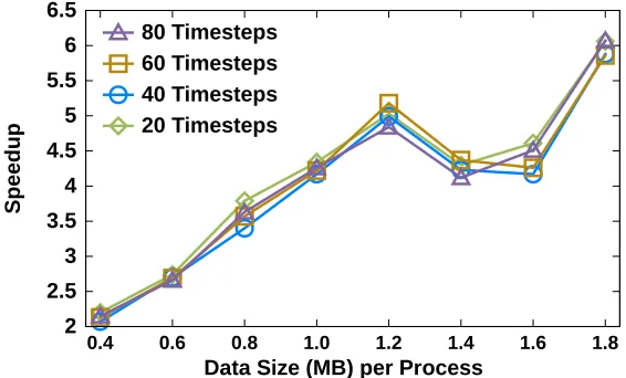
Speedup
Data Size (MB) per Process 20 Timesteps
40 Timesteps 60 Timesteps 80 Timesteps
Figure 2.7: Speedup ofPCCLoverAd Hoc 1in a BISICLES run where no calving occurs for many consecutive timesteps. Greater speedups are observed at larger per-process data sizes, as before. This speedup is consistent as more no-calving timesteps transpire.
process increases, the relative speedup of our method increases commensurately. There is slight dip in speedup around certain data sizes; we theorize that the AMR load balancing algorithm is distributing boxes in a more scattered fashion for these sizes, leading to slightly increased communication. Regardless, PCCL consistently yields speeups overAd Hoc 2, from 2x to 6x. Second, at a fixed data size per process, PCCL yields steady speedups (up to 6x) for more consecutive timesteps. The primary reason for these speedups is that our method admits an optimization. Before the global detection phase, candidate components can be quickly checked for viability as calved icebergs by testing the “groundedness” property. If all components on all levels are grounded, Phase II can be skipped entirely, as no floating components could be produced. This optimization is only made possible by our method; whereas, theAd Hoc 1
approach cannot support this optimization, as no components are available to check until the very end of its execution.
2.4.3
Packed Channel – Large-scale Chombo Benchmark
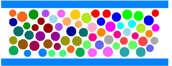
similar properties to the experimental medium such as porosity, tortuosity, and heterogeneity, effectively mimicking the natural material without the time-consuming process of imaging a real experiment. In turn, the results of this numerical simulation can be used to predict bulk parameters such as permeability, dispersivity, and reaction rates for better continuum scale models. We choose the packed channel for this set of experiments because the obstructions (filled circular regions) modeled within the channel form well-defined connected components, making them ideal candidates for detection with our algorithm (see Figure 2.8).
Figure 2.8: A depiction of a 2D packed channel dataset. The circular regions in the channel represent obstructions, with the remainder consisting of “pore space” through which fluid may flow. We color the circular regions, showing the connected components our method aims to detect.
Data preparation for the packed channel proceeds as follows. First, the initial data is gen-erated on a uniform mesh. We then apply a second tool to refine the grid at and within the boundary of the circular obstructions, to increase the resolution around these intricate surfaces. Next, the AMR mesh data is partitioned using Chombo’s actual load-balancing mechanism (“LoadBalance”), spreading the data across parallel processes. Finally, we invoke the con-nected component detection algorithm, which runs in a parallel,in situ context, exactly as if the data were generated in real time.
0 5 10 15 20 25 CP U T ime (s ec.)
Number of Processes
PCCL Ad Hoc 2 PCCL Ad Hoc 2 PCCL Ad Hoc 2 PCCL Ad Hoc 2 PCCL Ad Hoc 2
256 512 1024 2048 4096 Local ComputationCommunication Chombo Communication
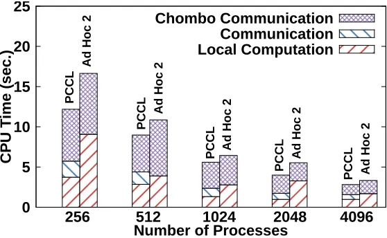
Figure 2.9: A timing breakdown comparison between PCCL and Ad Hoc 2 for an AMR dataset with 800 million total cells when run on Edison.PCCLachieves a consistent speedup overAd Hoc 2, up to 1.4x.
arately identified. Nonetheless,Ad Hoc 1is the closest analogue to our method we can find for comparison, so we adapt it to packed channel by removing the “grounding” constraint, terming the modified version “Ad Hoc 2.” Despite our method being “disadvantaged” by solving the harder, general version of the connected component detection problem, it still outperforms the special-purposeAd Hoc 2in the following results.
Figure 2.9 shows the performance comparison betweenPCCLandAd Hoc 2on the packed channel dataset (≈ 850 MB data) using a varying number of processes. PCCL is shown to achieve a consistent speedup Ad Hoc 2, up to 1.4x. A detailed breakdown of each method’s performance is also given, showing three timings:
• “Local Computation” includes core-local operations, primarily the local labeling algo-rithm (a fixed number of passes forPCCL, and iterative passes forAd Hoc 2).
• “Chombo Communication” consists of time to invoke Chombo’s built-in ghost cell com-munications, thefillInterpandexchangefunctions.
• “Communication” indicates any other communication induced by the method (onlyPCCL
invokes it, for aggregating and spreading label equivalence).