ABSTRACT
SOLTMANN, LARS MICHAEL. Determination of Power Required through Accelerated Flight with Application to Unmanned Vehicles. (Under the direction of Dr. Charles Hall.)
©Copyright 2016 by Lars Michael Soltmann
Determination of Power Required through Accelerated Flight with Application to Unmanned Vehicles
by
Lars Michael Soltmann
A dissertation submitted to the Graduate Faculty of North Carolina State University
in partial fulfillment of the requirements for the Degree of
Doctor of Philosophy
Aerospace Engineering
Raleigh, North Carolina 2016
APPROVED BY:
Dr. Ashok Gopalarathnam Dr. Scott Ferguson
DEDICATION
To my wife, Kimberly Soltmann. The sacrifices you have made in the interest of this research and my success as a graduate student mean more to me than you know. I am forever indebted
BIOGRAPHY
ACKNOWLEDGEMENTS
TABLE OF CONTENTS
List of Tables . . . vii
List of Figures . . . .viii
Nomenclature . . . x
Chapter 1 Introduction . . . 1
1.1 Motivation . . . 5
Chapter 2 Literature Review . . . 7
2.1 PIW-VIW Method . . . 7
2.2 W/δ Method . . . 9
2.3 Drag Polar Estimation . . . 11
2.4 Energy Approach . . . 15
Chapter 3 Theoretical Development . . . 17
3.1 Mathematical Model of an Aircraft . . . 17
3.2 Maximum Likelihood Estimation . . . 20
3.3 Power Required Analysis . . . 22
3.3.1 Aerodynamic Models . . . 23
3.3.2 Data Reduction . . . 23
Chapter 4 Flight Simulator. . . 27
4.1 Simulator Design . . . 27
4.2 Maneuver Selection . . . 28
4.3 Simulation of Pilot Input . . . 29
4.4 Noise Identification . . . 30
4.5 Simulation Results . . . 31
4.5.1 Case 1 - Validation and Near Ideal Runs . . . 31
4.5.2 Case 2 - Moderate Altitude Deviations . . . 34
4.5.3 Case 3 - Pitch Rate Assumption . . . 39
Chapter 5 Experimental Hardware Development . . . 43
5.1 Aircraft . . . 43
5.2 Data Acquisition System . . . 45
5.2.1 Data Requirements . . . 45
5.2.2 Hardware Design . . . 46
5.2.3 Software Design . . . 49
5.3 Five Port Probe . . . 51
5.3.1 Calibration . . . 53
5.3.2 Pressure Lag . . . 56
Chapter 7 Flight Test Results . . . 60
7.1 PIW-VIW . . . 60
7.2 Maximum Likelihood Results and Parameter Estimates . . . 61
7.2.1 Model Analysis . . . 66
7.2.2 Parameter Estimates . . . 68
7.3 Power Required . . . 70
7.3.1 Acceleration Runs . . . 72
7.3.2 Deceleration Runs . . . 76
Chapter 8 Conclusions. . . 78
8.1 Future Work . . . 79
References. . . 80
Appendix . . . 83
LIST OF TABLES
Table 3.1 Instrumentation error application . . . 24
Table 4.1 Bench test measured sensor noise variances . . . 31
Table 5.1 Dimensions for the Astraeus and Nexstar UAS . . . 45
Table 5.2 List of sensors on the flight data system . . . 47
Table 7.1 Parameter estimates under white Gaussian noise assumption . . . 69
LIST OF FIGURES
Figure 1.1 Free body diagram of an aircraft in steady, level, unaccelerated flight . . . 2
Figure 1.2 Power required and power available plot for the PLANK UAS . . . 5
Figure 2.1 One cycle of the pushover/pull-up technique . . . 12
Figure 2.2 Wind-up turn maneuver . . . 12
Figure 4.1 Overview of the flight simulator block diagram in Simulink . . . 28
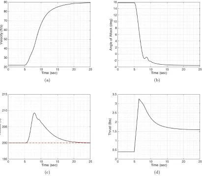
Figure 4.2 Flight simulator output for ideal deceleration run . . . 32
Figure 4.3 Maximum likelihood estimation output for ideal deceleration run . . . 33
Figure 4.4 Power required for ideal deceleration run . . . 34
Figure 4.5 Flight simulator output for near ideal acceleration run . . . 35
Figure 4.6 Maximum likelihood estimation output for near ideal acceleration run . . . . 36
Figure 4.7 Power required for near ideal acceleration run . . . 37
Figure 4.8 Altitude profile and estimated power required for the return to altitude case for an acceleration run . . . 37
Figure 4.9 Altitude profile and estimated power required for the return to altitude case for a deceleration run . . . 38
Figure 4.10 Altitude profile and estimated power required for the final altitude offset case for an acceleration run . . . 38
Figure 4.11 Altitude profile and estimated power required for the final altitude offset case for a deceleration run . . . 39
Figure 4.12 Flight simulator derived SNR cutoff for various system noise levels . . . 41
Figure 5.1 Astraeus UAS, high speed configuration . . . 44
Figure 5.2 Hobbico Nexstar . . . 44
Figure 5.3 ESC RPM output pulses, with and without decade counter . . . 48
Figure 5.4 Custom PCB for additional sensors, known as NavDAQ . . . 49
Figure 5.5 Assembled flight data system . . . 50
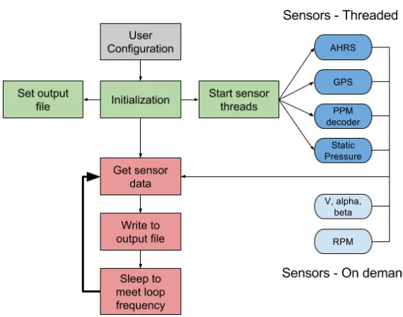
Figure 5.6 Data acquisition program flow chart . . . 50
Figure 5.7 Five port probe with labeled port numbers . . . 53
Figure 5.8 Five port probe test points used during calibration . . . 54
Figure 5.9 Angle of attack pressure coefficient versus angle of attack and side slip angle for all calibration velocities . . . 55
Figure 6.1 Flight test facility at Perkins Field . . . 57
Figure 7.1 Classic PIW-VIW flight test results: (a) Astraeus LS (b) Astraeus HS (c) Nexstar . . . 62
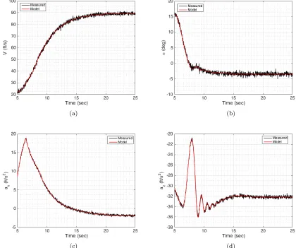
Figure 7.2 MLE velocity comparison with residuals for the Nexstar: (a) deceleration, (b) acceleration . . . 63
Figure 7.4 MLE axial acceleration comparison with residuals for the Nexstar: (a) decel-eration, (b) acceleration . . . 64 Figure 7.5 MLE vertical acceleration comparison with residuals for the Nexstar: (a)
deceleration, (b) acceleration . . . 64 Figure 7.6 MLE derived power required plot for the Nexstar with PIW-VIW
compari-son: (a) deceleration, (b) acceleration . . . 65 Figure 7.7 Power on noise comparison during an acceleration run for Astraeus and Nexstar 66 Figure 7.8 SNR values for measured flight data as well as simulated data . . . 67 Figure 7.9 Estimated lift and drag model parameter values and corresponding
confi-dence intervals . . . 68 Figure 7.10 Differences in model output when includingCLq for acceleration and
deceler-ation run on Nexstar: (a) velocity, (b) angle of attack, (c) axial accelerdeceler-ation, (d) vertical acceleration . . . 69 Figure 7.11 Dynamically generated power required results: (a) Astraeus LS (b) Astraeus
HS (c) Nexstar . . . 71 Figure 7.12 Flight simulator derived power required curves showing effect of system noise 73 Figure 7.13 Nexstar pitch response to a stepped vs ramped throttle input . . . 74 Figure 7.14 Throttle input: step vs ramp . . . 75 Figure 7.15 Power required comparison between stepped and ramped throttle input . . . 75 Figure 7.16 Final power required curves: (a) Astraeus LS (b) Astraeus HS (c) Nexstar . . 77 Figure A.1 Aeronaut CAM 12x8 wind tunnel test results: (a) thrust coefficient (b) power
coefficient (c) efficiency . . . 85 Figure A.2 APC 10x5 wind tunnel test results: (a) thrust coefficient (b) power coefficient
NOMENCLATURE
AR Aspect ratio
CD Drag coefficient
CDi Lift induced drag coefficient
CDW Wind axis drag coefficient
CD0 Zero lift drag coefficient
CL Lift coefficient
CL,minD Lift coefficient at minimum drag
CLq Lift due to pitch rate
CL0 Lift at reference condition
CLα Lift curve slope
CLδe Lift due to elevator angle
Cp Pressure coefficient
CX x-axis force coefficient
CY Side force coefficient
CYW Wind axis side force coefficient
CZ z-axis force coefficient
Cl Rolling moment coefficient
Cm Pitching moment coefficient
Cn Yawing moment coefficient
D Drag
D Dispersion matrix
Dprop Diameter of propeller
E Energy
F Force
I Moment of inertia
I Information matrix
J Cost
K Drag due to lift factor
L Lift
M Moment
M Mach number
N Total number of samples
P Power
P Pressure
R Noise covariance matrix
S Wing area
SE Sensitivity matrix
T Thrust
T Temperature
V Velocity
Ve Equivalent velocity
W Weight
X Matrix of regressors
Z Vector of measured outputs
a Acceleration
b Wing span
b0 Bias
cT Thrust coefficient ¯
c Mean aerodynamic chord
e Oswald efficiency factor
g Gravity
h Altitude
i, j, k Indices
le Length of tubing
m Mass
n0 Number of outputs
p Roll rate
q Pitch rate ¯
q Dynamic pressure
r Yaw rate
s Standard error
t Time
u, v, w Body axis velocities
x System states
y System output
z Measured output
Θ Vector of unknown parameters
α Angle of attack
β Angle of side slip
γ Heat capacity ratio
δe Elevator angle
δi,j Kronecker delta
θ Pitch angle
µ Coefficient of viscosity of air
ν Measurement noise
ξ Scale factor error
ρ Density
σ Air density ratio
σ2 Variance
φ Roll angle
ψ Yaw angle Superscript
T Transpose
−1 Inverse
. Time derivative
ˆ Estimate Subscript
A Available
sl Sea level
T Thrust
g Gravity
p Propulsion system
req Required
s Standard condition
t Test condition
x, y, z Cartesian coordinate axes Abbreviations
BHP Brake horsepower
P IW Power independent of weight
SN R Signal to noise ratio
T HP Thrust horsepower
Chapter 1
Introduction
Aircraft performance is one of the most important elements in the design and analysis of an aircraft. While it is a broad topic, covering areas such as take-off, landing, climb, etc., it is a good indicator of how successful an aircraft will be to its customers and its designed mission. One aspect of performance that has always received considerable attention is power required. Power required is defined as the power or energy per unit time necessary to sustain level, unaccelerated flight at a given velocity and altitude. This is an extremely important performance parameter that, along with the power plant, determines a number of other parameters such as maximum level speed, climb performance, flight efficiency, etc.
Estimation of the power required curve during the design phase, or as a theoretical eval-uation, is done through a drag analysis of the aircraft known as a drag build-up. To perform a drag build-up, the drag of individual vehicle components are estimated and summed to pro-duce an estimate of the overall vehicle drag [20]. These build-up methods provide ’ball park’ estimates but may not be entirely accurate. If a computational fluid dynamics (CFD) model of the aircraft exists, it can provide a much more accurate estimate of the overall vehicle drag and therefore, its power required. During the flight testing phase of a project it provides feedback to the designer on how well actual performance compares with designed and what the customer can actually expect in terms of overall performance.
espe-cially when it comes to size and weight. The testing methods developed throughout the history of aviation were done so mainly for manned aircraft although they can generally be applied to UAS without too many problems. However, in certain instances modifications can, or need to be made, so that the methods can be easily applied to UAS. In the case of power required analysis, the classic methods can be applied without issues but some changes can be made to increase accuracy or to incorporate technologies that were not available at the time the original method was developed. For example, the majority of small UAS are powered by electric motors which historically found little use in aircraft propulsion. Internal combustion engines were the most common power plants used so the methods were developed around their performance. Testing methods were also designed to be performed by the pilot who had direct visual, sensory, and instrumentation feedback. While most UAS today have telemetry feedback of some kind, some small vehicles as well as research aircraft are remotely piloted with little to no feedback. This can complicate following certain test procedures that require somewhat accurate knowledge of the current aircraft states. Therefore, new testing methods have been and will continue to be developed catering to the ever growing popularity of UAS.
In order to develop or improve methods in any field of study, an understanding of the basics is required. Power required is derived from the equations of motion governing steady level flight. Figure 1.1 shows a free body diagram for an aircraft in level, unaccelerated flight with the assumption that the thrust acts along the bodyx-axis. Summing the forces along the
Figure 1.1: Free body diagram of an aircraft in steady, level, unaccelerated flight
x and y axis yields
X
Fx= 0 =Tcos(α)−D (1.1)
X
whereT is thrust,Dis drag,W is weight,Lis lift, andαis the angle of attack. Assuming small angles, the equations along thex andy axis simplify to thrust is equal to drag and lift is equal to weight respectively. Applying the definition of power then gives the well known equation for power required to maintain flight at a given condition
P =F·V
Preq =DV =TreqV (1.3)
whereP is power,F is force, andV is velocity. This is the main equation that power analysis is based on in design, testing, and this research. This equation can be expressed in a few different ways that yields important characteristics about the power required curve. Assuming that an aircraft is in steady, level, unaccelerated flight and its drag model follows the form
CD =CD0+
CL2
πeAR (1.4)
whereCD is the drag coefficient,CD0 is the zero lift drag coefficient,CL is the lift coefficient,e is the Oswald efficiency factor, and ARis the wing aspect ratio. The definition of power from Eq. 1.3 can then be used to expand the power required equation to
Preq = 1 2ρV 3SC D0 + W2 1 2ρV S
πeAR (1.5)
whereρis the air density andS is the wing area. Taking the derivative with respect to velocity and setting it equal to zero yields
dPreq dV = 3 2ρV 2SC D0 − W2 1 2ρV2S
πeAR = 0
=3 2ρV
2S
CD0− 1 3CDi
= 0
CD0 = 1
3CDi (1.6)
whereCDi is the lift induced drag coefficient. Flight at this aerodynamic condition will achieve
along with the same drag model as before
Treq =D
Treq = 1 2ρV 2SC D0+ W2 1
2ρV2SπeAR
(1.7)
Taking the derivative with respect to velocity and setting it equal to zero yields
dTreq
dV =ρV SCD0−
4W2
ρV3SeπAR (1.8)
Simplifying the equation by making the substitution 4W2 ρ2V4S2 =C
2
L (1.9)
shows that the condition necessary for maximum range is
CD0 =
CL2
πeAR =CDi (1.10)
earlier marked, is shown in Figure 1.2. The difference between the power available and required curves shows the excess power available which provides information on the climb performance of the aircraft but will not be discussed here as it is outside the scope of this research.
Figure 1.2: Power required and power available plot for the PLANK UAS
1.1
Motivation
Chapter 2
Literature Review
Power required, or more specifically drag, has been heavily researched since the early days of aviation. Many of the estimation techniques were developed in the early part of the 20th century in an effort to make aircraft faster, more efficient, and to better understand overall performance. A majority of these techniques have been refined over the years as aircraft designs and technology have improved but are still applicable today and some are actively recognized by the FAA for use in aircraft certification [12].
2.1
PIW-VIW Method
the aircraft weights at two different conditions through the equation
Ws
Wt = Ls
Lt
= 0.5ρslσsV 2 sSCL 0.5ρslσtVt2SCL
(2.1)
whereσ is the air density ratio and the subscriptstandsrepresent the test and standard con-ditions respectively. Canceling like terms, solving forVs, and making the following substitution
Ve=Vt
√
σ (2.2)
whereVe is the equivalent velocity. Equivalent velocity is defined as the velocity at sea level in standard atmospheric conditions for which the dynamic pressure is the same as the dynamic pressure at the true airspeed and altitude at which the aircraft is flying. The equation for VIW is given as
V IW =Vs=
Ve
p
Wt/Ws
(2.3)
The second key assumption of the PIW-VIW method plays into the PIW term and assumes that the propeller efficiency is constant. For aircraft with constant speed propellers, this is a relatively safe assumption [12]. Through a mathematically similar approach as for the VIW term, the ratio of standard to test condition thrust horsepower (THP) is given as
T HPs
T HPt
= Vs 0.5ρslσSV 2 sS)
550
Vt 0.5ρslσtVt2S)
550 (2.4)
where the division by 550 is used to convert to horsepower. Using the constant propeller effi-ciency assumption, thrust horsepower can be replaced by brake horsepower (BHP) and substi-tuting VIW for Vs yields
P IW = BHPt
√
σt (Wt/Ws)1.5
(2.5)
Plotting PIW vs VIW provides the normalized power curve for the aircraft that can be used to determine the power under any weight and air density combination.
taken. Once steady state has been reached, airspeed, altitude, ambient temperature, RPM, manifold pressure, fuel quantity, fuel flow, and carburetor air temperature (if applicable) are recorded. Manifold pressure is then decreased by 1 inHg. Again, the airspeed must be allowed to stabilize before data can be recorded. This process is repeated until the back side of the power curve or stall is reached. The process is then repeated for different altitudes. The collected data is used in Eqs. 2.3 and 2.5 to determine VIW and PIW values for each test point. Since real measurements have noise associated with them, a normalization technique is used to transform the cubic power curve into a straight line for easy fitting. This is done by multiplying PIW by VIW and VIW by VIW3 giving
P IW ×V IW =m0V IW4+b0 (2.6) wherem0 and b0 are the slope and intercept, respectively, determined from the resulting plot. This technique was developed in the time before unmanned vehicles, but is still applicable. Depending on the type of vehicle this technique is applied to, slight modifications to the un-derlying equations and procedures are necessary. A detailed discussion of the changes can be found in Chapter 3. At this point it is evident that while this method is easy to perform and implement, it does have some drawbacks. The main drawback is that steady state conditions must be present for the PIW-VIW assumptions to be accurate. Since the phugoid mode requires a long wait time to be fully damped out, this causes the total test time to increase significantly. Also if any disturbances are encountered during this settling period, it may cause enough of an excitation that additional wait time is needed before accurate data can be taken. For manned or unmanned aircraft on a large test range where long runs of straight and level flight can be conducted, this does not present a problem. However, in a test range with limited space or where the aircraft has to remain within visual contact, this can present a problem. By the time the pilot needs to maneuver the aircraft to remain within the test range boundaries, most likely not enough time will have passed to have achieved steady state conditions, causing inaccurate data. Small aircraft are also more susceptible to atmospheric disturbances than larger aircraft making it much harder to maintain equilibrium conditions. The situation is further complicated by the fact that the aircraft states become harder for the pilot to discern as the distance between the pilot and aircraft increases.
2.2
W/δ
Method
be neglected. Standardizing flight data taken during high speed runs using the PIW-VIW flight test procedure and reduction method resulted in skewed data. To account for compressibility effects a pressure altitude reduction method, known as the W/δ method, can be used instead of a density reduction method. In this method the aircraft is flown at constant values of weight over the pressure ratioδ.
Starting with the drag model given by Eq. 1.4, both sides are multiplied by ¯qS to give drag
D=CD0qS¯ +
CL2qS¯
πeAR (2.7)
where ¯q is the free-stream dynamic pressure. Applying the lift equation (L=CLqS¯ ) under the assumption thatL=W results in
D=CD0qS¯ +
W2
πeARqS¯ (2.8)
The dynamic pressure can be written in terms of Mach number where
¯
q = 1 2γPtM
2 (2.9)
whereγ is the heat capacity ratio,P is pressure, andMis the Mach number. Substituting this equation into Eq. 2.8 results in
D= CD0(M)γPtM 2S
2 +
2W2 πe(M)ARγPtM2S
(2.10)
Both sides the equation are now multiplied by Psl
Pt whereby the pressure ratio is defined as
δ= Pt Psl
D δ =
CD0(M)γPslM2S
2 +
2 (W/δ)2
πe(M)ARγPslM2S
(2.11)
conditions. In this method, however, additional prior planning is needed to predict the aircraft weight over time to determine what altitudes need to be flown at each test point in order to maintain a constantW/δ. Timing during these flights is critical as spending too much time at one condition may burn too much fuel and make the aircraft too light for the next test point, changing the W/δ. Once the steady state condition has been reached, engine, velocity, and atmospheric data are recorded for post flight data reduction.
The majority of operational UAS, especially those in the private sector, operate in the very low subsonic region so this test method is not directly applicable. However, it does represent a method for drag/power determination. A low subsonic version of Eq. 2.11 can be written by starting with Eq. 2.8 and using the standard definition of the dynamic pressure along with the definition of density
ρ= P
RT (2.12)
where R is the universal gas constant and T is temperature. Using the same procedure as before, the low subsonic version of Eq. 2.11 can be rewritten as
D δ =
CD0PslV2S 2RT +
2RT (W/δ)2
πeARPslV2S (2.13) In this case the equation is a function ofW/δ, velocity, and temperature. Adding the tempera-ture adds an extra element of complexity especially during large altitude changes or long tests. While this method could be applied to low subsonic UAS, it is not as useful or as easy as the PIW-VIW method.
2.3
Drag Polar Estimation
While the PIW-VIW technique has the been the standard for many years, more modern tech-niques based on dynamic maneuvers have been developed as sensor and recording technologies have advanced. Since the power required is directly related to drag, the power required can be calculated if the drag polar can be determined. Estimating the drag polar from measured flight dynamics can be done in several ways. Many of these methods are based on model determina-tion through optimizadetermina-tion although some take a direct approach to solving for the drag through the equations of motion.
parameters. A more detailed discussion of the maximum likelihood estimation technique can be found in Chapter 3. A common maneuver used in drag polar estimation is the pushover/pull-up (roller coaster) maneuver, which is shown in Figure 2.1[5]. This maneuver is started by slowly
Figure 2.1: One cycle of the pushover/pull-up technique
pushing the nose of the aircraft down at constant rate of≈0.1 g/sec until a certain load factor (between -1 and 0) has been achieved. The nose is then pulled up at the same rate until a certain positive load factor has been achieved (usually 2) [5][24]. The load factor range covered during the maneuver should cover most of the lift coefficient range of the aircraft. At this point, which equations of motion are applied to the data varies depending on the models the user is trying to apply. Another maneuver that can be performed to achieve the same results is the wind-up turn, shown in Figure 2.2. In this maneuver, it is much easier to maintain velocity
Figure 2.2: Wind-up turn maneuver
to be included, as opposed to the pushover/pull-up maneuver where the wings remain level the entire time and the lateral dynamics can be safely ignored. A similar argument can be made here about the application of these maneuvers to UAS as was done with the PIW-VIW method. These maneuvers were designed for manned aircraft where the pilot has direct real-time feedback of the load factor. More advanced UAS will be able to have the autopilot perform these maneuvers without problem, but for those UAS that have a ground based pilot, maintaining a constant g-force rate will be difficult even if telemetry is available. This is especially true for the pushover/pull-up maneuver since it is conducted along a straight line meaning the aircraft will travel a significant distance by the end of the maneuver, most likely putting it out of visual range or outside of the test boundaries.
A majority of researchers who use these maneuvers determine the drag polar through the axial and vertical force models
CX =f(α, δe, V) (2.14)
CZ=f(α, δe, V) (2.15)
CD =−CXcosα−CZsinα (2.16) where CX and CZ are the force coefficients along their respective axes and are functions of various combinations and orders of the given state variables [5] [10]. The output of the equations of motion based on the above axial and vertical force models are compared against easily measurable aircraft parameters to determine model conformity. The most common measurable aircraft parameters used for comparison are [10] [19]
z= [q q˙ α V θ ax az]T (2.17)
where q is the pitch rate, θ is the pitch angle, and ais the acceleration along the given axis. The resulting drag polars have been compared to those obtained through wind tunnel testing and are in good agreement [5][10][13][24].
Another approach to drag polar estimation that is similar to maximum likelihood is estima-tion through least squares. Both techniques are optimal with respect to a given cost funcestima-tion, but their analysis process differs. In least squares it is assumed that the output is directly mea-surable along with the regressors. The only unknowns are the parameters for which the user applies a model and uses least squares regression to determine the unknown parameters based on the given model. The least squares model is given as
ˆ
Θ = XTX−1XTZ (2.18)
estimated parameters [19]. In reference 24, the authors make the assumption that lift and drag can be directly measured using the equations
CL=
nzaW −Tsinα 1
2γPtM2S
(2.19)
CD =
T−nxaW 1
2γPtM2S
(2.20)
wherenxa and nza are the longitudinal and vertical load factors respectively. The model to be estimated is
CD =CD0(M) +K1(M) +K2(M)CL2 (2.21) where CD0, K1, and K2 are the unknown parameters to be determined. Since this particular research investigated the drag polar throughout the transonic region, the unknown parameters were allowed to change with Mach number [24]. The same pushover/pull-up maneuver was used to generate a time history of the regressors with a suitable amount of information to accurately estimate the unknown parameters. The resulting drag polars are in good agreement with previous estimates for the aircraft. Although this research was conducted in the transonic and supersonic region, the above method could directly be applied to subsonic analysis by assuming that the unknown parameters remain constant with airspeed.
The equations of motion can also be used to directly calculate drag without using optimiza-tion. Care must be taken when using these methods because they do not include or make any assumptions about measurement noise. Using a free body diagram, the sum of the forces along the wind axes give the equation for drag as [13]
the same as the PIW-VIW method that provides only a single point on the drag polar. It is noted that the acceleration/deceleration maneuvers do not provide as many data points as the pushover/pull-up maneuver since they are not able to achieve the high lift coefficients at high velocities (M ≈1). Therefore, the pushover/pull-up and windup turn maneuvers are favored when a comprehensive characterization of the Mach number/drag relationship is desired [13]. The author also emphasizes that the pushover/pull-up maneuvers must be performed slowly so as not to violate the quasi-steady state assumption. The equations used do not contain pitch effects so they must be kept low in order to be considered negligible. Although the case is made here that the pushover/pull-up and windup turn maneuvers are favored over the accel-eration/deceleration runs, the opposite case could be made when applying these maneuvers to UAS. Acceleration/deceleration runs are much easier to perform by a ground based pilot and since the speeds are in the low subsonic region, the drag characterization with respect to Mach number is of no importance. Therefore, these runs can be used effectively in drag/power required analysis.
2.4
Energy Approach
Another approach to performance based flight testing that can be applied to drag estimation is energy analysis. Energy approaches are generally used in climb analysis of high performance aircraft but can be applied globally. The methods were originally formulated to deal with the change in true airspeed that occurs with large increases in altitude [12] [16]. In order to climb, an aircraft must have excess power, however, this excess power can also be used to accelerate instead of climb. The total energy of an aircraft in flight is given by the sum of the kinetic and potential energy as
E= 1 2mV
2+mgh (2.23)
whereE is energy,m is mass,gis the acceleration due to gravity, and his altitude. Taking the time derivative of the equation yields
˙
E=mVV˙ +mgh˙ (2.24)
Level or climbing acceleration is achieved when thrust is greater than drag so the first term in equation 2.24 can be rewritten and the equation becomes
˙
Chapter 3
Theoretical Development
The motion of an aircraft is a complex interaction between forces and moments involving many variables. Mathematically describing such complex systems in detail is generally difficult so model based approaches are used to describe the motion using simplified mathematics. The power required values for an aircraft that are most often presented are the steady state values. An aircraft is rarely at steady state conditions so the power required at any given time is generally not equal to the steady state value, but a combination of the steady state value plus some delta due to maneuvering. Determining the instantaneous total power required is trivial but finding the component solely due to maneuvering is not. Model based design provides a relatively easy way to determine how the individual parts of the system interact to determine what the base power required must be at any time. To do this, a mathematical description of an aircraft is necessary.
3.1
Mathematical Model of an Aircraft
The equations of motion for an aircraft have been well studied and only a brief derivation will be given here, highlighting the assumptions made to obtain the final equations. A detailed derivation can be found in reference 19. The derivation assumes a standard right hand coordinate system with the origin at the center of gravity and the x, y, z axes pointed forward through the nose, out the right wing, and through the underside respectively. This coordinate system is fixed on the aircraft and is known as the body-axis coordinate system. The assumptions made to start the derivation are as follows [19]
1. The aircraft is a rigid body with fixed mass distribution and constant mass, 2. The air is at rest relative to the earth,
4. The earth’s surface is assumed to be flat,
5. Gravity is uniform and does not change with altitude,
6. Thrust from the propulsion system acts along the bodyx-axis and through the center of gravity.
Using Newton’s second law of motion, the general motion of an aircraft can be described by the equations
Faero+Fg+FT =
d
dt(mV) =mV˙ +ω×mV (3.1) Maero=
d
dt(Iω) =Iω˙ +ω×Iω (3.2)
where
Faero= Fx Fy Fz = ¯qS
CX CY CZ
Maero=
Mx My Mz = ¯qS
bCl ¯ cCm bCn (3.3) ω= p q r
V =
u v w
I =
Ix −Ixy −Ixz
−Iyx Iy −Iyz
−Izx −Izy Iz
(3.4)
Fg=m gx gy gz body
FT = T 0 0
hp=
IpΩp 0 0 (3.5)
Within these definitions, ¯cis the mean aerodynamic chord,bis the wing span,M is the moment,
pis the roll rate,r is the yaw rate, Ωp is the propulsion system RPM, I is the mass moment of inertia,CY is the side force coefficient,Cl, Cm, Cnare the rolling, pitching, and yawing moment coefficients, andu, v, w are the body axis velocities. By substituting equations 3.3 through 3.5 into equations 3.1 and 3.2 and completing the necessary algebra, the final force and moment equations are obtained.
˙
u=rv−qw+qSC¯ X
m −gsin(θ) + T
m (3.6)
˙
v=pw−ru+qSC¯ Y
m +gcos(θ) sin(φ) (3.7)
˙
w=qu−pv+ qSC¯ Z
m +gcos(θ) cos(φ) (3.8)
˙
p−Ixz
Ix ˙
r = qSbC¯ l
Ix
− (Iz−Iy)
Ix
qr+ Ixz
Ix
qp (3.9)
˙
q= qSbC¯ m
Iy
−(Ix−Iz)
Iy
pr−Ixz
Iy
(p2−r2) +Ip
Iy
˙
r−Ixz
Iz ˙
p= qSbC¯ n
Iz
−(Iy−Ix)
Iz
pq−Ixz
Iz
qr−Ip
Iz
Ωpq (3.11)
The rotational kinematic equations are obtained by rotating the body axis rates into to the earth axes
˙
φ=p+ tanθ(qsinφ+rcosφ) (3.12) ˙
θ=qcosφ−rsinφ (3.13)
˙
ψ= qsinφ+rcosφ
cosθ (3.14)
where φis the roll angle and ψ is the yaw angle. The above nine equations (3.6 - 3.14) define the non-linear motion of an aircraft through the atmosphere based on the assumptions made at the beginning of the derivation. These equations were formulated in the body axis coordinate system and were used in the development of the flight simulator. In the analysis of flight test data the force equations are not quite as useful because the body axis velocities u, v, w cannot be directly measured. In this case, rotating the body axis coordinate system to align with the incoming relative wind vector allows for u, v, w to be expressed in terms of V, α, β, which are directly measurable. The body axis velocities are related to the wind axis through the equations
u=V cosαcosβ (3.15)
v=V sinβ (3.16)
w=V sinαcosβ (3.17)
V =pu2+v2+w2 (3.18)
The body axis velocities are also related to the angle of attack and side slip angle through the equations
α= tan−1
w
u
(3.19)
β = sin−1v
V
(3.20) Substituting equations 3.6 - 3.8 and 3.15 - 3.18 into equations 3.19 and 3.20 and performing the necessary algebra, the wind axis equations are given as
˙
V =−qS¯
mCDW +
T
mcosαcosβ+g(cosφcosθsinαcosβ
+ sinφcosθsinβ−sinθcosαcosβ)
˙
α=− qS¯
mV cosβCL+q−tanβ(pcosα+rsinα)−
Tsinα mV cosβ
+ g
V cosβ(cosφcosθcosα+ sinθsinα)
(3.22)
˙
β=− qS¯
mVCYW +psinα−rcosα+
g
V cosβsinφcosθ
+sinβ
V
gcosαsinθ−gsin cosφcosθ−Tcosα
m
(3.23)
where CDW and CYW are the wind axis drag and side force coefficients. If the side slip angles
are sufficiently small, CDW and CYW reduce to CD andCY.
All of the above equations can be used as they are or further simplified by linearizing them about an operating point by Taylor series expansion. Since the power required analysis conducted in this research was not done in real-time and had no computational restrictions, the full nonlinear equations were used. In addition, the aerodynamic model equations (section 3.3.1) must be defined before the equations can be used. The aerodynamic models in general depend nonlinearly on present and past values of airspeed, angle of attack, rotational rates, etc., therefore, their dependencies can be difficult to characterize [19].
3.2
Maximum Likelihood Estimation
Given a set of aircraft parameters, it is possible to accurately model the response of the aircraft using the equations of motion. In practice, however, the aircraft parameters are generally un-known but can be estimated through theoretical methods or flight data analysis. Given a time history of measured quantities from the vehicle response, unknown parameters can be chosen and adjusted to match the model output to the measured response. A common method for solving these types of problems is the maximum likelihood estimation technique. This tech-nique determines the value of unknown model parameters by maximizing the likelihood of a given measurement. This involves minimizing the weighted least squares difference between measured and model outputs [19]. Maximum likelihood methods for aircraft parameter iden-tification generally take on two forms: output-error method and equation-error method [19]. The key difference between the methods are how they handle noise. The output-error method assumes no process noise but includes measurement noise while the equation-error method as-sumes that process noise is present but with error free measurements of the states. The research described here focuses on the output-error formulation with the assumption that the noise is white, Gaussian, stationary, and uncorrelated.
motion can generally be described by a set of equations that take on the form
˙
x(t) =f
x, ui, t,Θˆ
(3.24)
y(t) =g
x, ui, t,Θˆ
(3.25)
z(t) =y(t) +ν(t) (3.26) where ˆΘ is the vector of unknown parameters, x is a vector of state variabels, y is a vector of the model outputs, z is a vector of measurements, ui is a vector of inputs, t is time, and
ν represents the measurement noise. Since this derivation focuses on the output-error method, the process noise is excluded. The measurement noise is assumed to be white with
E[ν(i)] = 0 (3.27)
E
h
ν(i)ν(j)T
i
=R(i)δij (3.28)
whereiandj are indices,R is the noise covariance matrix, andδij is the Kronecker delta. The likelihood function for a sequence of measurementsZN = [z(1)z(2) . . . z(N)]T can be written as L[ZN; Θ]. After successive applications of Bayes’s rule over N samples and assuming that the noise is uncorrelated and normally distributed [19],
L[ZN;θ] = N
Y
i=1
L[z(i); Θ] (3.29)
It is generally more advantageous to minimize the negative logarithm of the likelihood function than it is to maximize it. Since the log function is monotonic, this is permissible and provides an estimate of the unknown parameter
ˆ
Θ = min Θ
N
X
i=1
−ln{L[z(i); Θ]} (3.30)
The system noise can be described as the difference between the measured and model output (Eq. 3.26) and approaches a Gaussian distribution as the sample rate increases. Making this assumption, the negative log of the likelihood function, after some algebraic manipulation, becomes
−ln{L[z(i); Θ]}= 1 2
N
X
i=1
νT(i)R−1ν(i) +N
2 ln|R|+
N n0 2 ln(2π)
(3.31)
setting it equal to zero allows for the minimum error condition to be solved for. The resulting cost function J used to evaluate the model is given as
J(Θ) = 1 2
N
X
i=1
ν(i)T Rˆ−1ν(i) (3.32)
where
ˆ
R= 1
N
N
X
i=1
ν(i)ν(i)T (3.33)
ν(i) =z(i)−y(i) (3.34) The cost function is minimized using a relaxation technique where ˆR is computed and held constant while Eq. 3.32 is minimized with respect to Θ. The minimization of Θ can be done using any optimization technique chosen by the user. Once Θ has been minimized, ˆR is recalculated and the process is repeated until the change in the cost function from the previous iteration is below some user defined threshold [19].
3.3
Power Required Analysis
Now that the governing equations of the system and parameter estimation method have been defined, they can be combined to estimate the steady state power of the aircraft. The analysis that follows relies on two key assumptions
1. The pitching moment (pitch rate) at any given time is negligible. 2. The lateral dynamics at any given time are negligible.
3.3.1 Aerodynamic Models
For general analysis at low subsonic speeds with slow dynamics, linear aerodynamic models are sufficient. The aerodynamic models used in this research are given as follows
CL=CL0+CLαα+CLδeδe (3.35)
CD =CD0 +K(CL−CL,minD)2 (3.36) whereCL0 is the lift coefficient at the reference condition,CLαis the lift curve slope,CLδeis the lift due to elevator deflection,δeis the elevator angle,CL,minDis the lift coefficient at minimum drag, andK is the drag due to lift factor. The lift model generally includes the derivativeCLq,
the change in lift coefficient due to pitch rate, but due to the first assumption the term is left out. Some drag models also leave out the CL,minD term but, in general, the minimum drag of an aircraft does not occur at zero lift, but at some positive value so the term must be included [10]. The moment model (CM) is also not included because of the second assumption. Since the pitch rate is considered negligible, the longitudinal moments of the aircraft will be essentially zero.
3.3.2 Data Reduction
The aircraft states concerned with motion in the vertical plane are generally given as [5] [10]
x= V α q θ (3.37)
Since the pitch rate is assumed to be negligible, q and θ drop out making the state, output, and measurement vectors
x= " V α # y= V α ax az model z= V α ax az measured (3.38)
where the axial and vertical accelerations are given by the equations
ax=
CXqS¯ +T
Table 3.1: Instrumentation error application
Variable Bias Error Scale Factor Error
ax, az X —
α X X
V X X
az =
CZqS¯
m (3.40)
where
CX =CLsinα−CDcosα (3.41)
CZ =−CLcosα−CDsinα (3.42) It is important to note that Eq. 3.39 and Eq. 3.40 are written with respect to the center of gravity and do not include gravity. When comparing the equation outputs to the measured accelerometer data it is necessary to either remove gravity from the measurement or add it to the equation outputs since accelerometers cannot distinguish between gravity and pure accel-erations.
The measurements taken by the accelerometers, as well as other sensors, are subject to random as well as systemic errors. Systemic errors due to calibration errors, low quality sensors, inaccurate trim values, etc. can be compensated for by adding bias and scale factor parameters called nuisance parameters [19]. The measurement equation model, Eq. 3.26, with systemic instrumentation error can be written as
z(t) =ξy(t) +b0+ν(t) (3.43)
where ξ is the scale factor error and b0 is the bias error. Not all sensors require both scale factor and bias error corrections. Table 3.1 lists the type of error added for each variable. The nuisance parameters are estimated along with the parameters of interest, but their values are of no interest. They serve only as correction factors to allow for a better model fit.
Estimation of the lift and drag models begins by using the initial parameter values and initial measurements to solve the lift and drag models (Eq. 3.35 and 3.36) and then solving Eq. 3.21, 3.22, and Eq. 3.39 through 3.42. The state update equation
is used along with the sampling frequency to determine the aircraft’s states and outputs. The estimated outputs are then compared with the measured values, the parameter estimates up-dated accordingly, and the process is repeated. Once a feasible solution has been found, a new covariance matrix,R, is determined and the process repeated until the cost function (Eq. 3.32) no longer decreases. As previously mentioned, any optimization method can be chosen to mini-mize the cost function. For this research, the built-in MATLAB optimization functionfmincon was used, applying the default interior-point algorithm.
Once the iterative optimization process has successfully converged, the drag model was used to determine the true steady state power required curve for the aircraft using lift coefficient values corresponding to lift=weight at any given velocity. The power is then calculated using the equation
Preq=DV =CD0.5ρV3S (3.45) The power required values calculated are dependent upon the aircraft weight and atmospheric conditions present during the test. To remove these dependencies so that data from different tests and days can be compared, the same reduction procedure as outlined by the classic PIW-VIW method was used. In this case the actual power output is known, soBHP can be replaced by Preq and the equation becomes
P IW = Preq
√
σt (Wt/Ws)1.5
(3.46)
The dynamic method was compared against the classic method for validation since it is an accepted method for measuring power required. However, in this case some changes to the equations are needed. The classic method was designed around aircraft with reciprocating en-gines where the actual power output was unknown and could only be estimated. In this case, the actual power output from the motor/propeller combination is known. At any point in time the propulsion system power output is equal to
PA=T V (3.47)
The thrust from the propeller can be calculated using the equation
T =cTρΩ2pDprop4 (3.48)
A. Substituting the known power output for the estimated power, the PIW equation can be rewritten as
P IW = BHPT
√
σt (Wt/Ws)1.5
= T V
√
σt (Wt/Ws)1.5
(3.49)
The VIW equation remains the same where
V IW = p V
Wt/Ws
Chapter 4
Flight Simulator
4.1
Simulator Design
The flight simulator was designed to speed up development of the analysis method and to quickly test potential maneuver designs for effectiveness. The aerodynamic models from the previous chapter combined with the equations of motion provide the basis for the flight simu-lator. MATLAB Simulink was used to implement the simulator, which is shown in Figure 4.1. The aerodynamic models used in the flight simulator are based on those of the Astraeus UAS. Details about the aircraft can be found in Chapter 5. The models were derived from a combina-tion of theoretical analysis as well as previous flight test data. The simulator uses a fixed-step solver utilizing Euler’s method at 0.02 sec increments.
The Nonlinear Aircraft Model block in Figure 4.1 contains the nonlinear equations of motion and is the core block of the simulator. The equations of motion are contained in a function block that is looped back into itself to update the aircraft states. The states are updated according to Eq. 3.44. The initial conditions for the simulation are set in an external file by the user and include initial velocity and altitude. Since the simulator was setup to test maneuvers that start from a steady state condition with motion happening primarily in the vertical plane, the initial conditions solver automatically solves for the angle of attack and motor RPM to maintain steady level flight at the given condition.
The propulsion system block contains the propeller model for the aircraft based on wind tunnel testing. Several functions within the block control the RPM to provide an increasing throttle ramp, decreasing throttle ramp, manual input, or pass through from an outside con-troller input.
Figure 4.1: Overview of the flight simulator block diagram in Simulink
positioning. Simulated pilot input is achieved through manipulation of the PID gains within the controllers as well as through preprogrammed inputs. A detailed discussion on simulated pilot input is given later in this chapter.
The velocity control block is an optional block that allows the user to set a predetermined velocity profile or single target value. A PID controller varies the RPM in order to control the vehicle’s velocity. A model of the brushless motor used is included in the controller to more accurately model the motor’s response to any given input. The model was generated from physical testing during a previous project.
The last control block is the lateral control block. This block also contains PID controllers to actuate the ailerons and rudder based on the given target roll and yaw values. For this research the target values were always set to zero bank and zero yaw. In both the altitude/elev block and lateral control block, the control surface commands were sent through a servo model that was based on a model generated from physical testing on a similarly sized servo.
4.2
Maneuver Selection
propor-tional to drag, these maneuvers can also be used to determine power required. However, most of these maneuvers require relatively tight control and work well for manned and autonomous aircraft but not remotely piloted aircraft. The roller coaster maneuver requires the aircraft to slowly pitch up at a rate of 0.1 g/sec until 2 g and then nose over at -0.1 g/sec until 0 g is achieved. This is relatively easy for a skilled pilot sitting in the cockpit to perform and even easier for an autonomous aircraft. For a remotely piloted vehicle with no telemetry feedback, this maneuver is extremely difficult to perform as the pilot has no way of knowing the g-force rate. Similarly, the windup turn maneuver also requires a linear g-force increase in a constant altitude turn. Again, without feedback this is extremely difficult for a remote pilot to judge. The slow down maneuver starts with the aircraft in trimmed steady level flight and then sets the throttle to low or idle and allows the aircraft to naturally slow down while providing control input to maintain altitude and keep the wings level. This maneuver is much easier for a remote pilot to perform so it was selected as a candidate for testing. The inverse of this maneuver, starting at a low velocity and applying full power to accelerate at a constant altitude can also be used to determine the power required. If the thrust at every instant in time is known, then the thrust available can be determined and the aircraft’s acceleration will reflect the difference in available and required power of the system. This maneuver was selected as the second test candidate.
4.3
Simulation of Pilot Input
The simulator was not designed to operate in real time and, therefore, can not utilize actual pilot input during the maneuvers. However, several methods and models exist to simulate human response to tracking in non-real time systems [1] [8]. These models are fairly complex and more complicated than what is required in this case. Initial simulation runs of the acceleration and deceleration maneuvers have shown that the total run times are relatively short, less than 20 sec, and the response of the aircraft is of more importance than the pilot input. If the aircraft performs the maneuver without any deviation in the vertical plane, the power required can easily be determined by summing the forces along the x-axis. However, in reality no pilot, or even controller, will be able to perform the deceleration or acceleration maneuver perfectly. The goal of the simulations is to determine to what degree deviations are allowable before the method no longer provides reasonable results. Therefore, accurately modeling a human pilot is not essential.
in the ability to maintain altitude. As the distance between the aircraft and pilot increases, it becomes increasingly more difficult for the pilot to correctly judge the aircraft’s states such as climb rate, altitude, and bank angle. Therefore, some maneuvers may end up at a higher or lower altitude than they started, and/or with a gentle turn unintentionally executed somewhere during the maneuver. The simulator will test the method’s robustness using these deviations.
The two types of human control that were implemented in this simulator were those men-tioned above, poor gain values on the altitude PID controller and altitude following. A well tuned controller provides excellent control with very little deviation in altitude during the en-tire maneuver. Low gain values cause large but slow deviations from the target altitude which are undesired but keep the pitch rate low. High gain values cause small but quick deviations which hold altitude well but may violate the negligible pitch rate assumption. The gains can also be scheduled to provide a combination of these responses and more accurately simulate a pilot who is trying to maintain a constant altitude. Gain values were chosen on a trial and error basis since an optimal response was not required.
Altitude following uses a well tuned altitude controller to follow a preprogrammed altitude profile that mimics a human pilot. Altitude profiles from previous PIW-VIW and neutral point determination flights have shown that the target altitude profile can be expressed as the sum-mation of sine waves. The exact formulation is somewhat arbitrary and only needs to conform to a few loosely defined guidelines. The target profile should not have a dh/dt value whose magnitude is too large and the total altitude gain or loss, as well as the peak value, should also not be too large. The definition of too large is left to the user’s particular situation and will most likely be defined by the aircraft used in testing.
4.4
Noise Identification
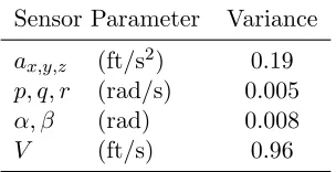
Table 4.1: Bench test measured sensor noise variances
Sensor Parameter Variance
ax,y,z (ft/s2) 0.19
p, q, r (rad/s) 0.005
α, β (rad) 0.008
V (ft/s) 0.96
white Gaussian.
4.5
Simulation Results
The simulation results are broken down into three cases: one to validate the simulator and power required reduction method, one to test scenarios likely to occur during the flight test phase, and one to investigate the negligible pitch rate assumption. All cases provide results for both the acceleration and deceleration runs as these will be the maneuvers used during the flight test phase. The first case covers the results from simulated pilot input that exhibits excellent altitude control. This represents a near perfect data run that was used to validate the simulator and data reduction methodology. The next case shows results for data runs where the pilot control was marginal and in one case finished at the same altitude (or very close to it) and in another case, finished at a higher or lower altitude. The last case investigated the assumption of negligible pitch rate and when it can and cannot be assumed to be negligible.
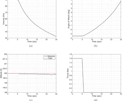
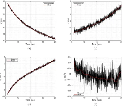
4.5.1 Case 1 - Validation and Near Ideal Runs
(a) (b)
(c) (d)
(a) (b)
(c) (d)
Figure 4.4: Power required for ideal deceleration run
4.5.2 Case 2 - Moderate Altitude Deviations
The cases shown here represent altitude deviation profiles that are likely to occur during flight testing. As previously mentioned, the distance between the pilot and aircraft will cause difficul-ties in judging altitude changes and whether or not the aircraft is at, or has been brought back to, the same altitude that it started from. It is likely that a sinusoidal oscillation around the target altitude will occur and that the starting and finishing altitudes will differ. The first set of results (Figure 4.8) shows an acceleration run where decaying oscillations around the target altitude occur. The power plot shows a very good match between the theoretical and estimated power curves. Figure 4.9 shows the same case but for a deceleration run. Here the amplitude of the altitude oscillations increased as the aircraft slowed down. Again, the power plot is in agreement with theory, but with a small deviation of around 2 ft-lbs/s in the middle of the velocity range. Several additional cases were run for both acceleration and deceleration runs in which the power required plots were all in agreement with theory.
(a) (b)
(c) (d)
(a) (b)
(c) (d)
Figure 4.7: Power required for near ideal acceleration run
(a) (b)
(a) (b)
Figure 4.9: Altitude profile and estimated power required for the return to altitude case for a deceleration run
(a) (b)
(a) (b)
Figure 4.11: Altitude profile and estimated power required for the final altitude offset case for a deceleration run
4.5.3 Case 3 - Pitch Rate Assumption
In Chapter 3, two key assumptions were made in the analysis development, one of which was that the pitch rate dependent terms can be considered negligible. The main reason for this assumption was that the maneuvers designed to be used with the analysis method are performed at a constant altitude where changes in the pitch angle and angle of attack occur very slowly over the duration of the maneuver causing a very low pitch rate. In the case of the ideal deceleration, the simulator shows a pitch angle change of about 8 deg over 20 sec, which equates to a pitch rate of 0.4 deg/s. This value is too low to measure based on the variance of the sensor noise. However, during the acceleration run the peak pitch rate was determined to be 6.8 deg/s, which is measurable even though this value can be considered negligible in this case. At some point however, the pitch rate can no longer be considered negligible, and must be included in the model. The analysis that follows determines the pitch rate limit.
The pitch rate affects the lift model, and therefore the drag model, directly through the derivative CLq. The significance and accuracy of this parameter, or any parameter for that matter, is determined by the information matrixI. The information matrix is defined as
I =−E
∂2lnL
∂Θ∂ΘT
(4.1)
but can be rewritten as
I =D−1 = N
X
i=1
using the assumptions made in the theoretical development where the dispersion matrix D is equal to the covariance matrix when the noise is white Gaussian and whereSEis the sensitivity matrix [18]. As the information content in the signal decreases, i.e. the signal-to-noise ratio of the pitch rate decreases, the information matrix becomes ill-conditioned causing the covariance estimate of the parameter to go to infinity through the inversion process. The magnitudes of the individual covariance values are used for testing parameter significance through hypothesis testing. In the case of pitch rate, the hypothesis for testing is given as
H0 :CLq = 0
H1 :CLq 6= 0 (4.3)
The t-statistic
t0= ˆ CLq s ˆ CLq (4.4) where
sCˆLq
≡
r
VarCˆLq
(4.5)
is used as the metric to determine whether or not the null hypothesis can be rejected [9]. If
|t0|> t(α∗/2, N −np) wherenp is the number of parameters, thenCLq is statistically different from zero. The value forα∗used in the tests is 0.05. Generally, in flight testing, the sample size is significantly greater than the number of model parameters such that the value oft(α∗/2, N−np) tends towards 1.96. For all of the simulator and flight test results this holds true, so 1.96 was used as the cutoff value.
Since the information content of the pitch rate signal will determine whether or not CLq is significant, it was the primary variable used for testing. Information content is directly related to signal magnitude. However, it alone is not sufficient to determine significance. Since the real world is not noise free, random noise must be accounted for as it has the possibility of ’drowning out’ a signal depending on its magnitude. The signal-to-noise ratio (SNR) is a much better variable for use in testing as it accounts for both. The signal-to-noise ratio is defined as
SN R= Psignal
Pnoise
(4.6)
However, in this analysis we can use an alternate form of the definition that is more useful. In the case of these maneuvers, the pitch rate is a zero mean signal and by definition the additive noise is as well, so the equation can be written in terms of variance instead of power
SN R= σ 2 signal
σ2 noise
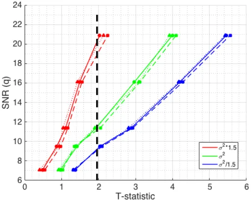
whereσ2 is the variance. For the simulated data, the SNR value is easily calculated because the two components that make up the final signal (true signal + additive noise) are known. For the flight test data, the variances are estimated using a different technique that is explained in detail in Chapter 7. In addition to the SNR effect on the significance of CLq, maneuver effects were also considered since reproducibility by the pilot can be difficult. Three different maneuvers were tested to determine what effect, if any, maneuver type had on the outcome. The three maneuvers used were those shown in Figures 4.9 through 4.11. For each test, the maneuver and magnitude of the noise on each output variable remained constant while the magnitude of the noise on the pitch rate signal was increased or decreased. Noise variance was based on the values in Table 4.1. The outputs were run through the maximum likelihood technique and the estimated value forCLq along with its variance were used in Eq. 4.4 to determine significance. During testing it was noted that the magnitude of the noise on all of the other parameters played a role in the significance ofCLq. Therefore, each maneuver was also run with all sensor noise values increased by 50% for the second case and decreased by 50% for the third case. The resulting SNR values for each maneuver and noise variance factor are shown in Figure 4.12. Within the plot, the different line types, solid, dashed, or dotted, represent the three different
Figure 4.12: Flight simulator derived SNR cutoff for various system noise levels
Chapter 5
Experimental Hardware
Development
5.1
Aircraft
Two aircraft were used in the validation of the dynamic power required analysis method, the Astraeus UAS and the Hobbico Nexstar. The Astraeus UAS was designed and constructed by the 2010/2011 Aerospace Engineering senior design class as a reconfigurable multi-purpose UAS. Design requirements dictated that a high speed and low speed configuration sharing a common fuselage and empennage be designed with specific stall speed requirements for each configuration. To this end, the aircraft was an excellent candidate for use as a test bed for method validation, because the UAS has two different wings. The power required for the entire aircraft changes depending on which wing is currently being flown. Thus, two different power required curves can be generated without moving the data system from one vehicle to another. The high speed version is shown in Figure 5.1. The payload section of the aircraft was originally designed for a fairly large avionics box allowing for plenty of room for a small data collection system with separate power supply. Only a single modification to the payload section was necessary to receive the new avionics tray which consisted of four mounting holes in the forward and aft section. The pitot-static tube was also replaced with a custom five port probe for angle of attack and side slip measurements. The construction and calibration of this probe is detailed in section 5.3.
Figure 5.1: Astraeus UAS, high speed configuration
Table 5.1: Dimensions for the Astraeus and Nexstar UAS
Parameter Astraeus(LowSpeed) Astraeus(HighSpeed) Nexstar
b, ft 7.75 5.5 5.73
¯
c, ft 0.753 0.793 0.870
S, ft2 5.81 4.35 4.99
CGx, ft* 0.390 0.342 0.277
W, lbs 6.57 5.83 8.47
*Measured along the wing root airfoil.
controller were also upgraded to compensate for the increased weight due to the addition of the flight computer and supporting hardware and extra flight batteries. Table 5.1 gives the relevant dimensions of both Astraeus and the Nexstar.
5.2
Data Acquisition System
The design of the data collection system went through several iterations based on the data requirements of the method, available sensors, currently available systems, and previous expe-rience with other systems.
5.2.1 Data Requirements
To utilize the analysis method described in Chapter 3, the data system must record certain flight parameters. The parameters, shown in the list below, are those needed to solve Equations 3.21, 3.22, 3.35, 3.39, and 3.40.
T V ax az ∆t p q r α β δe θ φ
These parameters are needed for the power required analysis utilizing accelerating or decelerat-ing runs. However, since the classic PIW-VIW method was also performed, an additional flight parameter was needed, namely ˙h. A direct measurement of this value can be obtained through GPS, but it can also be determined from an altitude profile. Therefore,hand ˙hwere also added to the data requirements list.
frequency. In an environment where multiple frequencies of interest exist, the data acquisition system must be set to sample at a rate of at least twice the highest frequency of interest [26]. For aircraft dynamics, the mode that generally exhibits the highest frequency is the short period mode. While this research is not directly interested in measuring the short period mode, several parameters such as angle of attack and pitch angle, are affected by this mode, and these quantities are used in the underlying equations. For the Astraeus UAS, the short period mode is 1.1 Hz. Data on the dynamics of the Nexstar does not exist but since it is comparable in size, shape, and weight, it is assumed that its short period mode is of similar frequency. Therefore, the minimum sampling frequency to avoid aliasing is 2.2 Hz. However, while this ensures that the signal can be recovered, a good reconstruction of the signal will require more points. It is generally suggested to sample at a rate of 10 times the highest frequency to obtain enough points for a good reconstruction [11]. Using these requirements and guidelines, the data system sample rate was set at 25 Hz.
5.2.2 Hardware Design
Table 5.2: List of sensors on the flight data system
NAVIO Sensors Data Collected
MPU9250 ax, ay, az, p, q, r, θ, φ, ψ
u-blox M8 GPS NED velocity, altitude, position, course MS5611 barometric altitude and temperature Additional Sensors Needed
Differential pressure transducers (3) Angle of attack, side slip angle, airspeed Absolute pressure transducer altitude
Microcontroller RPM
The NAVIO shield contains most of the sensors needed to meet the data requirements but not all. Table 5.2 contains a list of the sensors contained on the NAVIO as well as the additional sensors needed. Although the NAVIO already contains an absolute pressure transducer, it does not have a hose barb and lacks the ability to mount one on it, so a second transducer with a hose barb was added. Unless specific provisions are made to ensure that the pressure inside of the fuselage is equal to static pressure, a separate static measurement must be made.
Instead of mounting the additional sensors on separate breakout board(s) away from the Raspberry Pi, an additional shield with the extra sensors was designed to be mounted between the Raspberry Pi and NAVIO. This saves space and weight and decreases the complexity of the design. Before the sensors shield could be designed, the exact make/model of the extra sensors needed to be identified. The angle of attack and side slip sensors were chosen based on the the five port probed design requirements and is detailed in section 5.3. The sensor chosen for both angle of attack and side slip measurements was the Measurement Specialities MS4515DO with a sensing range of±2 inH2O and an accuracy of 0.25% full span.
The airspeed sensor was chosen based on previous flight test data collected on Astraeus. During flight testing, the maximum speed observed was 103 ft/s on either configuration, which equates to a dynamic pressure of 2.4 inH2O under standard conditions. Ideally, a sensor whose range is the same as that observed during testing would be chosen, but no digital differential sensors with a range around 2.4 inH2O could be sourced. A digital type sensor, specifically one using the I2C protocol, was chosen over an analog sensor because of the ease of use, simplified circuit layout, and reduced sensitivity to interference. The sensor chosen to measure airspeed was the Honeywell SSCDRRN005ND2A5, which has a sensing range of±5 inH2O and a 0.25% full scale span error.