Development of a Cell-Centred Finite Difference Numerical Methodology on Triangulated Domains

(1)

University of Windsor University of Windsor

Scholarship at UWindsor

Electronic Theses and Dissertations Theses, Dissertations, and Major Papers

2012

Development of a Cell-Centred Finite Difference Numerical

Methodology on Triangulated Domains

James Situ

University of Windsor

Follow this and additional works at: https://scholar.uwindsor.ca/etd

Recommended Citation Recommended Citation

Situ, James, "Development of a Cell-Centred Finite Difference Numerical Methodology on Triangulated Domains" (2012). Electronic Theses and Dissertations. 210.

https://scholar.uwindsor.ca/etd/210

This online database contains the full-text of PhD dissertations and Masters’ theses of University of Windsor students from 1954 forward. These documents are made available for personal study and research purposes only, in accordance with the Canadian Copyright Act and the Creative Commons license—CC BY-NC-ND (Attribution, Non-Commercial, No Derivative Works). Under this license, works must always be attributed to the copyright holder (original author), cannot be used for any commercial purposes, and may not be altered. Any other use would require the permission of the copyright holder. Students may inquire about withdrawing their dissertation and/or thesis from this database. For additional inquiries, please contact the repository administrator via email

(2)

Development of a Cell-Centred Finite Difference

Numerical Methodology on Triangulated Domains

by

JAMES J. SITU

A Thesis

Submitted to the Faculty of Graduate Studies

through Mechanical, Automotive and Materials Engineering

in partial fulfillment of the requirements for

the Degree of Master of Applied Science at the

Title Page

Windsor, Ontario, Canada

2011

(3)

James Jianmin Situ

(4)

Development of a Cell-Centred Finite Difference Numerical Methodology on

Triangulated Domains

by

James J. Situ

Approval Page

APPROVED BY:

_____________________________________________________ Dr. M.S. Monfared, External Department Reader

Department of Mathematics and Statistics University of Windsor

_____________________________________________________ Dr. N.G. Zamani, Internal Department Reader

Department of Mechanical, Automotive and Materials Engineering University of Windsor

_____________________________________________________ Dr. R.M. Barron, Advisor

Department of Mechanical, Automotive and Materials Engineering / Department of Mathematics and Statistics

_____________________________________________________ Dr. V. Stoilov, Chair of Defence

(5)

iv

Author’s Declaration of Originality

I, James Jianmin Situ, hereby certify that I am the sole author of this thesis. This thesis

includes original research that has been previously published/submitted for publication in

peer reviewed conference proceedings, as follows,

Thesis Chapter Publication title/full citation Publication status

Chapter 2 & 4 Situ, J.J. and Barron, R.M. Development of a Cell-Centred Finite Difference Scheme for Numerical Simulations on Triangulated

Domains. 19th Annual Conf. of the CFD

Society of Canada, Montreal, April 2011.

Presented

Chapter 2 & 4 Situ, J.J. and Barron, R.M. Cell-Centred Finite Numerical Methodology for Solving Partial Differential Equations on Triangulated

Domains. Applied Mathematics, Modeling and

Computational Science Conference, Waterloo, July 2011.

Under review

I certify that the above material describes work completed during my registration as a

graduate student at the University of Windsor.

I declare that, to the best of my knowledge, my thesis does not infringe upon anyone’s

copyright nor violate any proprietary rights and that any ideas, techniques, quotations, or

any other material from the work of other people included in my thesis, published or

otherwise, are fully acknowledged in accordance with the standard referencing practices.

Furthermore, I certify that I have not included copyrighted material that surpasses the

bounds of fair dealing within the meaning of the Canada Copyright Act.

Provisional Patent Application 61/457,589 has been filed on April 22, 2011 for Patent

Protection for: “Cell-Centered Finite Difference Method for Numerical Solution of

Partial Differential Equations on Arbitrary Mesh Systems”

I declare that this is a true copy of my thesis, including any final revisions, as approved

by my thesis committee and the Graduate Studies office, and that this thesis has not been

(6)

v

Abstract

A cell-centred finite difference (CCFD) method for unstructured mesh topology is

proposed and applied to model partial differential equations (PDEs) governing fluid flow

and solid mechanics phenomena. The numerical method implements a finite difference

approximation at cell centroids by taking differencing points along orthogonal Cartesian

axes localized within each cell. The predominant advantage of this method is that it can

be applied to arbitrary mesh topologies, including structured, unstructured and hybrid

meshes. Either a direct or iterative approach is used to solve the system of equations

developed by the proposed method. The numerical method is designed to solve a variety

of physical phenomena governed by PDEs, such as electrostatic potential in

electromagnetic fields, stress and strain in structural mechanics and wave phenomena in

physics. The focus of the thesis research is to investigate the application of this

methodology in heat transfer and fluid mechanics problems. This new finite difference

methodology is applied to typical “benchmark” problems in such fields, covering the

representative of different types of PDEs with initial and boundary conditions. Solutions

obtained are compared to exact solutions if available from analytical methods or to the

(7)

vi

Acknowledgement

It is a pleasure to thank many people who made this thesis possible.

I am indebted in the preparation of this thesis to my supervisor, Dr. Ronald M. Barron of

University of Windsor, whose patience and kindness as well as his indepth academic

knowledge, have been invaluable to me. With his enthusiasm, his inspiration and his

great efforts to explain concepts effectively, he helped me expand my knowledge greatly

in the engineering numerical analysis field. Throughout the period of writing this thesis,

he provided encouragement, advice and lots of innovative ideas. Without him, I would

not have been able to complete my thesis.

I would like to thank my committee members, Dr. Nader G. Zamani and Dr. Mehdi S.

Monfared, who are always available to provide support to my research when I needed it.

Also, lots of constructive suggestions from their feedbacks help improve the quality of

my thesis.

Lastly but not least, I wish to thank many friends, and especially my parents, who give

(8)

vii

Table of Contents

TITLE PAGE ... I COPYRIGHT PAGE ... II APPROVAL PAGE ... III AUTHOR’S DECLARATION OF ORIGINALITY ... IV ABSTRACT ... V ACKNOWLEDGEMENT ... VI TABLE OF CONTENTS ... VII LIST OF FIGURES ... X LIST OF TABLES ... XII NOMENCLATURE ... XIII

CHAPTER 1 – OVERVIEW OF PARTIAL DIFFERENTIAL EQUATIONS AND NUMERICAL TECHNIQUES ... 1

1.1 PRELIMINARY CONCEPTS OF PARTIAL DIFFERENTIAL EQUATIONS ... 1

1.2 CLASSIFICATION OF PDES ... 1

1.3 ANALYTICAL SOLUTION METHOD ... 2

1.4 EXPERIMENTAL SOLUTION METHOD ... 3

1.5 NUMERICAL SOLUTION METHOD ... 3

1.5.1 Finite Difference Method ... 3

1.5.2 Finite Volume Method ... 4

1.5.3 Finite Element Method ... 5

1.5.4 Mesh-Free Numerical Method ... 5

1.6 THESIS OVERVIEW ... 6

CHAPTER 2 – DEVELOPMENT OF CCFD NUMERICAL METHOD ... 7

2.1 ALGORITHM FOR PDENUMERICAL METHOD ... 7

2.2 IMPLEMENTATION OF FINITE DIFFERENCE FORMULA IN CCFDNUMERICAL SCHEME ... 7

2.3 FDSTENCIL POLYNOMIAL TRANSFORMATION ... 8

2.4 EVALUATING DIFFERENCING POINTS ... 10

2.4.1 Approximation Scheme at Interior Line Segment ... 12

2.4.1.1 End Node Weighted Average Approximation ... 12

2.4.1.2 Approximation by Interior Triangular Interpolation Function ... 13

2.4.1.3 Centroid and Nodal Weighted Average Approximation ... 14

2.4.1.4 Approximation by Quadrilateral Interpolation Function ... 15

2.4.2 Differencing Points Evaluated at a Dirichlet Boundary... 16

2.4.3 Differencing Points Evaluated at a Neumann Boundary ... 17

2.4.3.1 First-Order Backward Differencing Approximation ... 17

2.4.3.2 Second-Order Backward Differencing Approximation ... 18

2.5 CENTRAL FINITE DIFFERENCING AT CELL CENTROID ... 19

(9)

viii

2.7 DEVELOPMENT OF SYSTEM OF EQUATIONS ... 21

2.8 SUMMARY OF CCFDFORMULATION ... 22

CHAPTER 3 – PRELIMINARY OVERVIEW ... 23

3.1 MESH OVERVIEW ... 23

3.1.1 Mesh Quality ... 23

3.1.2 Mesh Classification ... 24

3.1.2.1 Conformality ... 25

3.1.2.2 Surface or Body Alignment ... 25

3.1.2.3 Mesh Topology ... 26

3.1.2.4 Mesh Element ... 27

3.2 SOLUTION OF SYSTEM OF EQUATIONS ... 27

3.2.1 Direct Solvers ... 27

3.2.2 Iterative Solvers ... 28

3.2.2.1 Jacobi Iterative Method ... 28

3.2.2.2 Gauss-Seidel Iterative Method ... 29

3.2.2.3 Successive Over-Relaxation (SOR) Iterative Method ... 30

3.3 MANUFACTURED SOLUTIONS ... 31

3.4 INTERPOLATION LINE POST-PROCESSING ... 31

3.5 ASSESSMENT CRITERIA ... 33

3.6 VARIATIONS OF CCFDNUMERICAL METHOD ... 33

CHAPTER 4 – APPLICATIONS TO PDES GOVERNING PHYSICAL PHENOMENA ... 34

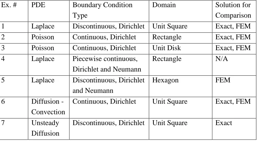
4.1 OVERVIEW OF BENCHMARKED EXAMPLES ... 34

4.1.1 Unit Square Discretisation ... 35

4.2 EXAMPLE 1:LAPLACE EQUATION WITH DISCONTINUOUS BOUNDARY CONDITIONS ... 36

4.2.1 Direct CCFD Approach ... 38

4.2.2 FEM Solution ... 41

4.2.3 Numerical Solution by CCFD Method ... 42

4.3 EXAMPLE 2:POISSON EQUATION IN A RECTANGLE WITH DIRICHLET BC ... 48

4.3.1 Numerical Solution by FEM ... 49

4.3.2 CCFD Solution ... 50

4.4 EXAMPLE 3:POISSON EQUATION IN A DISK WITH DIRICHLET CONDITIONS ... 51

4.4.1 Solution by FEM ... 53

4.4.2 Solution by CCFD ... 54

4.5 EXAMPLE 4:LAPLACE EQUATION FOR POTENTIAL FLUID FLOW ... 56

4.6 EXAMPLE 5:HEAT TRANSFER IN HEXAGONAL DOMAIN ... 59

4.6.1 FEM Solution ... 62

4.7 EXAMPLE 6:DIFFUSION-CONVECTION IN A UNIT SQUARE WITH DIRICHLET BC ... 65

4.8 EXAMPLE 7:UNSTEADY DIFFUSION IN A UNIT SQUARE WITH DIRICHLET BC ... 69

(10)

ix

5.1 DISCUSSION OF CCFDRESULTS ... 74

5.2 ERROR AND UNCERTAINTIES ANALYSIS ... 74

5.3 ADVANTAGE OF CCFDNUMERICAL METHOD ... 76

5.4 CCFDMETHOD FUTURE IMPROVEMENT ... 77

5.5 CONCLUSIONS ... 78

REFERENCES ... 79

APPENDIX A – MATLAB PDE TOOLBOX OVERVIEW ... 80

APPENDIX B – CCFD PROGRAM CODE OVERVIEW ... 81

APPENDIX C – DATA STORAGE ALLOCATION ... 83

(11)

x

List of Figures

Figure 2.1 Algorithmic process for solving PDE by numerical method ... 7

Figure 2.2 Differencing points in second order central FD stencil ... 8

Figure 2.3 Quadratic map transformation ... 9

Figure 2.4 Process of evaluating a differencing point ... 11

Figure 2.5 Parametric representation of a line segment AB ... 12

Figure 2.6 Differencing point approximation ... 14

Figure 2.7 Quadrilateral interpolation scheme ... 15

Figure 2.8 Four nodal quadrilateral element and master element [10] ... 16

Figure 2.9 Normal gradient in Neumann boundary bondition ... 17

Figure 2.10 2nd order and 4th order finite difference scheme ... 18

Figure 2.11 Process of forming system of equations by CCFD scheme ... 22

Figure 3.1 Non-conformal mesh ... 25

Figure 3.2 Examples of surface aligned and non-surface aligned meshes ... 26

Figure 3.3 Micro-structured, micro-unstructured and macro-unstructured, micro-structured meshes ... 26

Figure 3.4 Iteration process of Jacobi method ... 29

Figure 3.5 Iteration process of Gauss-Seidel method ... 29

Figure 3.6 Interpolation points for post-processing ... 32

Figure 4.1 Coarse mesh and refined mesh ... 35

Figure 4.2 Quality of coarse and refined meshes ... 36

Figure 4.3 Example 1 – Description ... 36

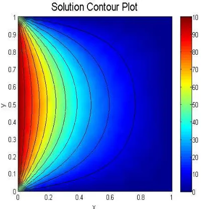
Figure 4.4 Example 1 – Analytical solution contour plot ... 37

Figure 4.5 Example #1 – Mesh #1... 38

Figure 4.6 Example #1 – Mesh 2... 39

Figure 4.7 Example 1 – FEM RE contour plots on coarse and refined meshes ... 41

Figure 4.8 Example 1 – CCFD solution contour plots on coarse and refined meshes ... 42

Figure 4.9 Example 1 – CCFD RE contour plots on coarse and refined meshes ... 43

Figure 4.10 Example 1 – Comparison of exact, FE and CCFD solutions along y = 0.05 on coarse and refined meshes ... 44

Figure 4.13 Example 1 – Absolute error contour plots on coarse and refined mesh ... 46

Figure 4.15 Example 2 – Contour plot of analytical solution ... 48

Figure 4.16 Example 2 – Mesh discretisation ... 49

Figure 4.17 Example 2 – Mesh quality in coarse and refined discretisation ... 49

Figure 4.18 Example 2 – FEM RE contour plots on coarse and refined meshes... 50

Figure 4.19 Example 2 – CCFD solution contour plots on both coarse and refined meshes ... 50

Figure 4.20 Example 2 – CCFD RE contour plots on coarse and refined meshes ... 51

Figure 4.21 Example 2 – AE contour plots in both coarse and refined meshes ... 51

(12)

xi

Figure 4.24 Example 3 – Coarse and refined mesh quality ... 53

Figure 4.25 Example 3 – FEM RE contour plots on coarse and refined meshes... 54

Figure 4.26 Example 3 – CCFD solution contour plots on coarse and refined meshes ... 54

Figure 4.27 Example 3 – RE contour plots on coarse and refined meshes ... 55

Figure 4.28 Example 3 – AE contour plots on coarse and refined meshes ... 56

Figure 4.30 Example 4 – Mesh discretisation ... 57

Figure 4.31 Example 4 – CCFD stream function contours by approximation scheme a) ... 58

Figure 4.32 Example 4 – CCFD stream function contours by approximation scheme b) ... 58

Figure 4.33 Example 4 – CCFD stream function contours by approximation scheme c) ... 58

Figure 4.35 Example 5 – Coarse, clustered and refined mesh topologies ... 60

Figure 4.36 Example 5 – Quality of coarse, clustered and refined meshes ... 60

Figure 4.37 Example 5 – Coarse, clustered and refined meshes in half model ... 61

Figure 4.38 Example 5 – Coarse, clustered and refined meshes in quarter model ... 61

Figure 4.39 Example 5 – Full model FEM solution contours on coarse, clustered and refined meshes ... 62

Figure 4.40 Example 5 – Half model FEM solution contours on coarse, clustered and refined meshes ... 62

Figure 4.41 Example 5 – Quarter model FEM solution contours on coarse, clustered and refined meshes 62 Figure 4.42 Example 5 – Full model RD on coarse, clustered and refined meshes ... 64

Figure 4.43 Example 5 – Half model RD on coarse, clustered and refined meshes ... 64

Figure 4.44 Example 5 – Quarter model RD on coarse, clustered and refined meshes ... 64

Figure 4.45 Example 6 – Exact solution contours for different P values ... 66

Figure 4.46 Example 6 – RE contours for P = 10 on coarse and refined meshes ... 68

Figure 4.47 Example 6 – RE contours for P = 40 on coarse and refined meshes ... 68

Figure 4.48 Example 6 – RE contours for P = 100 on coarse and refined meshes... 68

Figure 4.49 Example 7 – RE contours on coarse mesh with time step sizes of 20, 10, 5 and 2.5 ms ... 71

Figure 4.50 Example 7 – RD contours on coarse mesh with time step sizes of 20, 10, 5 and 2.5ms ... 72

Figure 4.51 Example 7 – RE contours on refined mesh with time step sizes of 20, 10, 5 and 2.5ms ... 73

Figure 4.52 Example 7 – RE contours 0n refined mesh with time step sizes of 20, 10, 5 and 2.5ms ... 73

Figure 5.1 Fishbone diagram of errors and uncertainties analysis ... 75

Figure 5.2 Neumann boundary not aligned with Cartesian axes ... 78

(13)

xii

List of Tables

Table 4.1 Application examples list ... 34

Table 4.2 Coefficients of CCFD equations for mesh 1 ... 38

Table 4.3 Coefficients of CCFD equations for mesh 2 ... 40

Table 4.4 FEM results for Example 1 ... 41

Table 4.5 Performance of CCFD solver for Example 1 ... 42

Table 4.6 Effect of relaxation parameter (coarse mesh) ... 46

Table 4.7 Effect of relaxation parameter (refined mesh) ... 47

Table 4.8 Example 2 – General result by FEM solver ... 49

Table 4.9 Example 2 – General result by CCFD solver ... 50

Table 4.10 Example 3 – General result by FEM solver ... 53

Table 4.12 Example 5 – Mesh information ... 60

Table 4.13 Example 5 – Half model and quarter model mesh information ... 61

(14)

xiii

Nomenclature

CC Cell centroid; cell centre

IP Interpolation point

OA Order of accuracy

RE Relative error

RD Relative difference

RMSE Root mean square error

RMSD Root mean square difference

SOR Successive over-relaxation scheme

ζ Spatial coordinate in computational stencil η Spatial coordinate in computational stencil

ai Coefficients of polynomial transformation from x to ζ

bi Coefficients of polynomial transformation from y to η

γi Coefficients in finite difference equation ω Relaxation parameter

For all points

Interior of a domain Boundary of a domain

Union of sets

Dependent variable at node/cell centroid index i at kth iteration

Exact value at index i

kth spatial derivative of Φ with respect to x at node/cell centroid index i

kth time derivative of Φ at time step n g(x,y) Neumann boundary condition function

x _{Independent variable}

y _{Independent variable}

(15)

xiv

t _{Time variable}

Ni Test function

Wi Weight function

Ni(x,y) Shape function

L Operator

α General differencing point index

S South differencing point

N North differencing point

W West differencing point

E East differencing point

M Mid differencing point

LAB Distance between two points A and B

(16)

1

CHAPTER 1 – OVERVIEW OF PARTIAL DIFFERENTIAL EQUATIONS AND

NUMERICAL TECHNIQUES

Partial differential equations (PDEs) arise in connection with various thermofluid and

solid mechanics problems. The governing PDEs are derived from physical principles and

lead to initial and boundary value problems in both time and spatial domains.

1.1 Preliminary Concepts of Partial Differential Equations

A partial differential equation is defined as an equation involving one or more partial

derivatives of a function of two or more independent variables. The order of the highest

derivative is called the order of the equation [1]. The solution of a PDE in a domain is

a function that has all partial derivatives appearing in the equation and satisfies the

equation everywhere in . However, a solution of a PDE is generally not unique. A

unique solution may be obtained by the use of additional information imposed by the

physical conditions, i.e. boundary conditions that give the values of the required solution

on the boundary and/or initial conditions that prescribe the value of the solution at initial

time t = 0. Some mathematical theorems describe the criteria for solution existence and

uniqueness of linear PDEs, but these theorems do not generally apply to nonlinear PDEs.

1.2 Classification of PDEs

A PDE for the function (x1,..xn) has the form

(1.1)

The PDE is linear if it is of the first degree in the dependent variable and its partial

derivatives . The independent variables xi’s can represent spatial

coordinates, time or other physical parameters, such as pressure, temperature, etc. A

nonlinear PDE contains the product of the dependent variable with itself or one of its

derivatives. If each term of the equation (1.1) contains either the dependent variable or

one of its derivatives, the equation is said to be homogeneous; otherwise it is said to be

(17)

2

In addition to the distinction between linear and nonlinear PDEs, further classification of

PDEs is essential for computational scientists and engineers working on numerical

simulation. Linear, second order PDEs can be classified as parabolic, hyperbolic or

elliptic based on the characteristic curves associated with the equation. Consider the

following second order linear PDE

(1.2)

Discontinuities in the second order derivatives of the dependent variable may arise across

the characteristics. Characteristic curves can be real or imaginary depending on the

discriminant value of the second order derivative coefficients. The second order PDE (1.2)

is classified according to the sign of the expression (B2 – 4AC) as follows:

1. Elliptic if B2 – 4AC < 0. An elliptic PDE has no real characteristic curves and any

disturbance is propagated instantly in all direction within the region [2]. The

solution domain is a closed region. This type of PDE usually arises in physical

application of diffusion processes into an equilibrium state, such as a steady state

temperature distribution or fluid motion at subsonic speed.

2. Parabolic if B2 – 4AC = 0. The solution domain is an open region and such PDEs

only exhibit one characteristic curve. The solution marches downstream within

the domain from prescribed initial conditions while satisfying the specified

boundary conditions [2]. For a physical interpretation, parabolic PDEs arise in

time-dependent diffusion problems, such as unsteady heat conduction.

Mathematically, parabolic PDEs serve as a transition from hyperbolic PDEs to

elliptic PDEs.

3. Hyperbolic if B2 – 4AC > 0. A hyperbolic PDE has two real characteristic curves

and the solution domain exhibits a disconnected conic section. Hyperbolic PDEs

usually arise in connection with mechanical oscillations, such as a vibrating string

or plate, or in convection driven transport problems.

1.3 Analytical Solution Method

Although analytical solutions for most PDEs are not obvious and may not even exist,

(18)

3

general analytical approaches to solve such PDEs include separation of variables,

conformal mapping, infinite series, coordinate and dependent variable transformations

and perturbation methods. Analytical solutions are available for some of the problems

considered in this thesis, and will be used as needed.

1.4 Experimental Solution Method

Experiments, as an alternative to numerical simulation, are often used for validation of

simulation results for a physical problem governed by PDEs. Experimental fluid

mechanics provides information regarding a particular flow field and thus experimental

data is used along with computational solutions of the equations for design purposes.

Nevertheless, limitations on hardware, such as wind tunnel size and measurement

resolution, sometimes make it impractical to perform an experiment. Huge costs may also

be encountered and some experiments are not possible to conduct, such as solar or

galactic events and nuclear explosions. For these reasons, numerical simulations are used

by engineers to reconstruct the physical condition under the appropriate boundary and

initial conditions.

1.5 Numerical Solution Method

Numerical methods specify a finite discretized domain from the continuum physical

domain and each finite discretization unit is analyzed individually. From a numerical

methods perspective, there are three well-established primary methodologies for solving

PDEs in a pre-defined mesh topology; finite difference, finite volume and finite element

methods. Finite difference (FD) and finite element (FE) methods are usually applied in

solid or fluid mechanics, while the finite volume (FV) method is popular in fluid

mechanics. Lohner [3] has classified the three numerical methods by choice of the trial

and test functions Ni and Wi based on a weighted residual formula.

1.5.1 Finite Difference Method

The FD method takes Ni as a polynomial and Wi = δ(xi), where δ is the delta function,

such that the operator approximation is enforced at a finite number of locations in

(19)

4

stencil of the operation. The traditional FD methods are commonly used in

Computational Fluid Dynamics (CFD) for problems that exhibit a moderate degree of

geometrical complexity, or within multiblock solvers. The discretization stencils are

derived for structured grids with uniform element size h. For this reason, for complex

geometries, FD methods usually require transformation from an arbitrary physical

domain to a structured and uniform computational domain.

1.5.2 Finite Volume Method

The FV (and FE) methodologies on the other hand have the capability of handling

unstructured or hybrid mesh systems. Most commercial and research CFD codes for

solving fluid flow and heat transfer problems are based on the FV methodology because

of the clear relationship between the numerical algorithm and the underlying physical

conservation principle [3]. The FV method employs integration of the governing

equations over all finite control volumes of the domain. In Lohner’s definition, FV

methods are obtained by taking polynomial Ni and Wi = 1 if integration is within the

element and 0 otherwise. Since the test function is set in Kronecker delta form in each of

the respective elements, any integration by parts over the control volume reduces to

element boundary integrals. This implies that only the normal fluxes through the element

faces appear in the discretization [4]. However, discretization in the time domain for

time-dependent problems is one of the limitations in FV because of global conservation.

Some revised FV techniques handle this problem, such as the integrated space-time (IST)

FV method proposed by Zwart [5]. In his dissertation, a space-time meshing algorithm

and a solver were developed for the IST FV method. Particular application of this method

is when conservation in time is important, such as moving boundary problems involved

free surface flow. Other limitations involve the development of higher-order methods,

such as the use of compact Hermitian schemes available in a FD formulation.

Higher-order methods are particularly important where very high solution accuracy is needed,

such as in computational aeroacoustics and direct numerical simulation of turbulent flows.

It is also difficult to implement the FV method on higher-order PDEs. One popular

(20)

5

a pass over the mesh and then obtain the next order derivative in the subsequent pass,

until the highest-order derivative has been reached [4].

1.5.3 Finite Element Method

In comparison, the FE method develops an equilibrium equation by inputting element

shape functions into the weak formulation of the PDEs. The FE method can be

summarized as the projection of the weak form of the differential equation onto a

finite-dimensional function space, as a combination of linear piecewise basis functions [5]. In

Lohner’s definition of the Galerkin FE method, the polynomial trial function Ni

is set to

be the test function, i.e. Ni = Wi [4]. This method is widely used for thermal problems,

structural dynamics, potential flows and electrostatics. However, special treatments are

needed to ensure a conservative solution. Lube and Rapin [6] presented different

techniques to handle the mass conservation in advection-diffusion problems, such as

higher-order approximations and constructing Scott-Vogelius elements. Surana et al. [7]

presented k-version of the FE method in gas dynamics for higher-order global

differentiability numerical solutions. The article addressed a FE approximation scheme of

differential equations by space-time coupled processes in order to preserve the physics

and mathematics of the initial/boundary value problem.

1.5.4 Mesh-Free Numerical Method

Besides the numerical methods based on a pre-generated mesh structure, there are

methods that do not require mesh generation, such as smoothing particle hydrodynamics

(SPH) and material particle semi-implicit (MPS) formulations. Regarding the SPH

method, it was developed to avoid the limitation of mesh tangling encountered in extreme

deformation problems. Absence of grid generation is the major advantage for the SPH

formulation compared to the traditional ALE (Arbitrary-Lagrangian-Eulerian)

formulation used in many fluid-structure problems. The SPH technique allows to obtain

numerical solutions of the continuum equations by defining the variables at a set of

suitable moving points and reconstructing the continuous field by means of interpolation

functions centred on each moving points [8]. However, there are limited actual

(21)

6

fluid-strucutre interaction problems with large deformation. It has difficulty to capture

turbulence effect in high Reynolds number flows. Also, some drawbacks need to be

further investigated, such as uneven particle distribution determined by characteristic

length and inter-particle distance discrepancies caused by large variations [9].

1.6 Thesis Overview

In the present research work, a cell-centred finite difference (CCFD) method is developed

for 2D arbitrary unstructured and hybrid mesh topologies. The primary objective of this

thesis is to develop the necessary equations, discuss the important features of the method

and demonstrate its potential applicability. Chapter 2 describes the algorithmic

development of the methodology and formulation of specific approximation schemes.

Chapter 3 provides a preliminary overview of related subjects, including mesh topology

information, methods of solving systems of equations, manufacturing of solutions,

assessment criteria for the CCFD method and post-processing interpolation. Chapter 4

applies the developed formulation to benchmarked two-dimensional PDE problems with

Dirichlet and Neumann boundary conditions, covering a spectrum of typical equations

and boundary conditions with different geometric domains. The last chapter summarizes

all the findings, analyzes sources of error and concludes with proposed future

(22)

7

CHAPTER 2 – DEVELOPMENT OF CCFD NUMERICAL METHOD

2.1 Algorithm for PDE Numerical Method

Specific numerical methods for PDEs involve formulation of the problem in particular

differential equation forms. The FE method develops the weak form of the differential

equation onto a finite-dimensional space, while the FV method applies integration over

the finite control volume based on laws of conservation of mass, momentum and energy.

The formulation is then applied to a predefined mesh structure or particles over the

interior domain. This leads to solving a system of algebraic equations to reach the final

solutions, either by direct or iterative methods. The general numerical process is shown in

the following figure:

PDE Problem Definition

Mesh Discretsation

Applying Boundary/Initial

Conditions

Applying Formulation on Predefined Mesh

Structure

Solving by Iterative Method

Solving by Direct Method

Solution Converge?

Final Solution Yes

No Updating Solution

Numerical Method Formulation

Developing System of Equations

Figure 2.1 Algorithmic process for solving PDE by numerical method

The CCFD formulation is first tested by direct scheme using Gaussian elimination in a

predefined simple mesh structure. Once results are validated by comparing to the exact

solution, an arbitrary mesh topology can be solved by Jacobi iterative scheme. Point

Gauss-Seidel and Successive Over-Relaxation (SOR) methods are also used to further

improve the convergence rate.

2.2 Implementation of Finite Difference Formula in CCFD Numerical Scheme

In the CCFD method, the PDE is evaluated at the centroid of each cell. Second order

partial derivatives are approximated using a central finite difference formula at the cell

centre. The order of accuracy of the differencing formulae depends on the number of

(23)

8

differencing at a cell centroid in the spatial domain, the expression for the second

derivative with respect to x is

(2.1)

where the y value is held constant, i.e., y = yj. Equation (2.1) approximates the second

order derivative at (xi, yj) by taking forward and backward differencing point values at

(xi+1, yj) and (xi–1, yj) and is of the order of O(Δx)2, provided the points (xi+1, yj), (xi, yj)

and (xi–1, yj) are equally spaced. For derivatives with respect to y, a similar finite

difference approximation is applied. In the CCFD formulation, the finite differencing

points are confined to remain within each cell. This can be achieved by setting up a local

Cartesian system with cell centroid at the origin and differencing points at the

intersection between the axes and cell edges. The figure below illustrates the localized

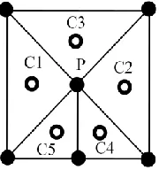
finite difference stencil in an element ΔABC:

Figure 2.2 Differencing points in second order central FD stencil

The differencing points are denoted as west (W), east (E), south (S) and north (N) relative

to the cell centroid, following the usual notation of the FV method.

2.3 FD Stencil Polynomial Transformation

Equation (2.1) presented in the previous section requires equally spaced grid points.

However, in general, for the numerical procedure depicted in Fig. 2.2, the differencing

point locations on a FD stencil are not uniformly distributed, eg., length of line segment

from CC to W is not the same as from CC to E. For this reason, a transformation is

(24)

9

one can use the polynomial transformation which maps the spatial variables

independently and is expressed by the following equations:

(2.2)

The coefficients s and s depend on the coordinates of the differencing points

referenced to a fixed global coordinate system, and localized Cartesian axes are aligned

along each FD stencil. The order n of the polynomial expression depends on the order of

approximation for each cell-centred finite difference expression. For example,

second-order central differencing at the cell centre requires a quadratic transformation, while a

fourth-order FD scheme uses a quartic transformation. The polynomial mapping is

applied to the PDE as well as the FD stencil, i.e., the PDE is transformed from the (x, y)

physical domain to the (ζ, η) computational domain. The major advantage of

implementing this polynomial transformation is that the same order of accuracy can be

maintained in the (ζ, η) FD equation as in the original (x, y) FD approximation formula.

Let’s consider second-order central FD scheme in a 2D steady problem. Quadratic

transformation is sufficient to bring physical coordinates (x, y) into the

computational coordinates (ζ, η) with equally spaced grid points. The origin in the local

Cartesian plane is set at the cell centroid and all the differencing points are mapped

within a unit square domain in a localized computational stencil (ζ, η). The quadratic

transformation maps the three differencing points in each direction independently, i.e. W,

CC and E in x-direction and S, CC and N in y-direction. The transformation of the stencil

is illustrated in the following figure:

(25)

10

By substituting the coordinates of the differencing points into the transformation

equations (2.2) in quadratic form (n = 2), the coefficients are determined as follows:

(2.3)

Similarly, a fourth-order central differencing approximation at the cell centroid employs a

quartic transformation. Five differencing points are taken in each direction, which are

classified as W, MW, CC, ME and E in x-direction and S, MS, CC, MN and N in y

-direction. The coefficients of the transformation are determined by substitution of the

differencing points’ coordinates into eqn. (2.2) in quartic form (n = 4) and the result in x

-direction transformation is:

(2.4)

Coefficients in y-direction have corresponding pattern with E replaced by N and W by S,

which gives,

(2.5)

2.4 Evaluating Differencing Points

A system of equations is to be developed from the finite difference formulation of the

(26)

11

discretised domain. In addition to parameter inputs, the values of the dependent variables

at the differencing points will be needed during the calculations. These values are

expressed in terms of neighbouring nodal values or cell centroid values, or a combination

of both. The locations of the differencing points for each cell are determined first. There

are three different possibilities where a differencing point might lies: at an interior edge,

coinciding exactly at an interior node, or at a boundary edge or boundary node. To

determine a differencing point condition, the boundary and the interior domain are

identified first. If a differencing point lies at a Dirichlet boundary, it is evaluated directly

from the specified boundary value. On the other hand, differencing points that lie on a

Neumann boundary are evaluated by the Neumann boundary point approximation scheme,

which will be discussed in section 2.7. For differencing points located in the interior

domain, the value of the dependent variable is expressed in terms of nodal and centroid

values based on an approximation scheme (discussed in section 2.4.1), if it is located on a

line segment. If a differencing point coincides at an interior node, then the nodal value is

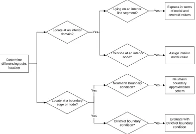
assigned to the differencing point. The following figure illustrates the process of

evaluating a differencing point:

Determine differencing point

location

Locate at an interior domain?

Locate at a boundary edge or node?

Yes

Assign interior nodal value Coincide at an interior

node? Lying on an interior

line segment?

Yes

Yes Yes

Express in terms of nodal and centroid values Dirichlet boundary condition? Neumann Boundary condition? Yes Evaluate with Dirichlet boundary condition Yes Neumann boundary approximation schem Yes

(27)

12

Parametric equations are used to determine if a differencing point lies on a line segment.

In Fig. 2.5, the relationship between a differencing point α and a line segment AB can be

expressed as

Figure 2.5 Parametric representation of a line segment AB

(2.6)

where represents any differencing point in any cell, and LAα and LBα are distances from

to A and B, respectively. Each differencing point in the interior domain is checked

using these parametric equations to determine its location relative to the nodes and edges

of the cell being considered, and its value is evaluated accordingly based on the process

chart, Fig 2.4 above.

2.4.1 Approximation Scheme at Interior Line Segment

If a differencing point lies at an interior line segment, it must be expressed in terms of

nodal and centroid values based on some approximation scheme. The approximation can

be solely confined within the cell or accompanied with effect from the neighbouring cell.

Several approximation schemes are illustrated in the following sections.

2.4.1.1 End Node Weighted Average Approximation

The value at a differencing point in a finite stencil can be evaluated by a weighted

average of the two end nodal values on an edge where the differencing point lies. In this

approximation scheme, values at differencing points are solely determined within the cell.

The general formula for this approximation scheme can be represented as a piecewise

(28)

13

(2.7)

where t is determined from parametric equations (2.6) This approximation using the

length-weighted average of the two end nodal values on the line segment is first order

accurate. In this case, the entire computation is confined within the cell. However,

neighbouring effects from boundary conditions and/or adjacent cells have no direct

influence in approximating differencing point values. Thus, the inaccuracy in this

approximation scheme has more significant effect when a discontinuity arises or large

gradient takes place. The results of the approximation will be discussed with examples in

later sections.

2.4.1.2 Approximation by Interior Triangular Interpolation Function

To perform approximation within the cell, a three-point triangular interpolation function

can be developed to evaluate differencing point values. The method is taken from the

finite element numerical method in approximating a functional value at an arbitrary point

within a cell, using the following equation [10]

(2.8)

where the variable are the nodal values and the functions Ni(x, y) are referred to as

shape functions that depend on the geometry of a cell. In the first-order triangular

element, the shape functions are determined as follows

(29)

14

where (i,j,k) is the cyclic permutation of (1,2,3) for the nodal index of a triangle and i≠j

≠ k, and A is the area of the triangle. In this approximation scheme, differencing point

value at a cell boundary (i.e. lying on an interior line segment) has the same value as

computed by the length-weighted average of end nodal values in the previous

approximation scheme discussed in section 2.4.1.1. Nevertheless, function values at

points that lie in the interior region of the cell generally have better approximation than

the length-weighted average scheme. This method is especially beneficial to approximate

higher-order derivative terms or higher-order accurate approximations for low order

derivatives that involve differencing points in the interior region of the cell.

2.4.1.3 Centroid and Nodal Weighted Average Approximation

In order to consider the neighbouring effect in approximating the differencing point

values, both inscribed and adjacent cell centroid values are taken into account in addition

to the two end nodal values. Location of the differencing point on a line segment is

determined by the parametric equation (2.6). Each interior line segment will have two

cells attached to it and both cell centroid values are used in the approximation of the

differencing point value. The approximation scheme is illustrated in the following figure

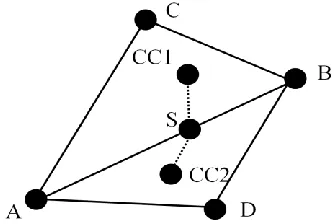
for a differencing point S lying on a line segment AB.

Figure 2.6 Differencing point approximation

Figure 2.6 considers the south differencing point S for ∆ABC. The south point lies on the

line segment AB and ∆ABD is the adjacent triangle with the common edge AB. In this

approximation scheme, four distances are required; distances to the two end nodes LAS

(30)

15

length-weighted average formula as eqn. (2.7) is used to approximate the function value

at the differencing point lying on an interior line segment:

(2.10)

Recall that if the differencing point locates at a node instead of on the line segment, the

nodal value is assigned to the differencing point. In this approximation scheme, the

adjacent centroid value is included in the evaluation of the differencing point to account

for the neighbouring cell effect. In general, such an approximation scheme is more

accurate than the two end node weighted average scheme, as demonstrated in later

examples.

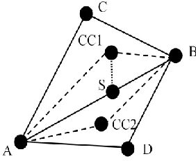
2.4.1.4 Approximation by Quadrilateral Interpolation Function

For better accuracy to approximate a differencing point value, a quadrilateral

interpolation function can be constructed by taking the two edge end nodes, inscribed

centroid and adjacent centroid as vertices. This approximation scheme is illustrated in Fig.

2.7.

Figure 2.7 Quadrilateral interpolation scheme

In this figure, the south differencing point of ∆ABC is taken as an example. The

quadrilateral constructed to evaluate the south point involves two end nodes, A and B, as

well as two centroids CC1 and CC2. The value at the differencing point is determined

from equation (2.8) as a linear combination of interpolation functions. Because of the

(31)

16

quadrilateral element to a unit square master element with origin at the centroid, which is

illustrated in Fig. 2.8.

Figure 2.8 Four nodal quadrilateral element and master element [10]

The interpolation functions can be simply constructed in the master element as:

(2.11)

The idea behind the mapping is to transform (x, y) domain into (s, t) master domain by

the following equations,

(2.12)

Given the coordinates (x, y) of the differencing point, new coordinates (s, t) in the master

domain are required to be determined from equation (2.12). The system of equations is

nonlinear, involving two equations and two unknowns. Extensive computation is needed

to calculate the new coordinate (s, t) of the differencing point. Thus, this approximation

scheme will not be investigated in the current research. Once having the differencing

point coordinates determined in the master element, the differencing point value can be

determined in a similar way as eqn. (2.8):

(2.13)

2.4.2 Differencing Points Evaluated at a Dirichlet Boundary

The values of the dependent variables at points that lie on a boundary on which Dirichlet

(32)

17

Dirichlet boundary conditions may represent streamfunction or velocity values in fluid

mechanics or temperature distribution in heat transfer. In solid mechanics, zero Dirichlet

boundary condition can be interpreted as the boundary being clamped without

displacement under loading conditions. If a differencing point lies at a Dirichlet boundary,

it is directly evaluated from the Dirichlet boundary condition based on its position.

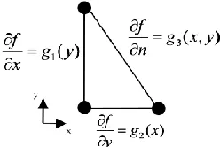
2.4.3 Differencing Points Evaluated at a Neumann Boundary

The Neumann boundary condition involves specification of the value of the first

derivative at the boundary. In thermal-fluid applications, Neumann boundary conditions

represent flux across the boundary, while it represents distributing load in solid

mechanics.

Figure 2.9 Normal gradient in Neumann boundary bondition

In Fig. 2.9, a Neumann boundary condition in a right triangle is taken to illustrate the

procedure. Normal gradients, ∂f/∂x and ∂f/∂y on the two edges are included in the

consideration since the Neumann boundaries are along one of the Cartesian axes. The

normal gradient on the hypotenuse, on the other hand, involves components in x- and y

-direction and the formulation for this kind of Neumann boundary condition is not

included in this thesis.

For Neumann boundaries aligned with the Cartesian axis, the function value at the

differencing point can be approximated by first-order or second-order one-sided finite

difference approximation schemes.

2.4.3.1 First-Order Backward Differencing Approximation

To illustrate the procedure, suppose the east differencing point lies on a Neumann

boundary. As a simple approximation, the first derivative can be evaluated by a

(33)

18

adjacent differencing point in the finite stencil. The first-order backward difference

formula in x-direction is

(2.14)

Since the Neumann boundary condition is along the x-axis, the normal gradient

can be expressed as a function of y, g1(y). Then the value for fij can be written as

(2.15)

Note that fi-1,j represents the backward differencing point value. In a second-order central

FD stencil, fi-1,j can be defined as the centroid value, while fi-1,j represents the adjacent mid

differencing point in a fourth-order central FD stencil. Similar formulae can be used to

approximate the normal gradient to the y-direction by substituting into

the backward finite difference equation.

2.4.3.2 Second-Order Backward Differencing Approximation

For a more accurate approximation, a second-order three-point backward finite

differencing scheme can be used to approximate the value at differencing points lying on

a Neumann boundary. The second-order backward differencing formula in x-direction is

(2.16)

Note that fi-1,j and fi-2,j represent the adjacent backward differencing point value. In the

second-order central differencing scheme on the finite stencil, fi–1,j represents the value at

the cell centroid and fi–2,j is the differencing point value intersecting at an interior edge

along the differencing direction. In a fourth-order central differencing on the finite stencil,

fi–1,j represents the mid differencing point and fi–2,j represents the cell centroid value along

the differencing direction. The figure below illustrates the second-order and fourth-order

central differencing within a cell.

(34)

19

Note that the spacing Δx between two neighbouring points are equal after the finite

stencil polynomial transformation, which was mentioned in section 2.3. Given the normal

gradient function value as , the equation (2.16) can be rearranged to solve

for fij as the following

(2.17)

For the differencing points lying on a Neumann boundary perpendicular to the y-axis,

similar formulae apply. Generally, the second-order backward differencing

approximation scheme is more accurate than the first-order approximation.

2.5 Central Finite Differencing at Cell Centroid

Once differencing points have been determined within each cell, the cell centroid value

can be evaluated by applying the governing PDEs at the cell centroid and using an

appropriate finite difference formula on the Cartesian system in the computation domain.

The governing PDEs are rewritten in terms of computational coordinates (ζ, η) which are

related to the physical coordinates (x, y) by the polynomial transformation discussed in

section 2.3. The general second order PDEs in (1.2) can be rewritten in terms of ζ and η

as:

(2.18)

where the coefficients etc., depend on the metrics of the transformation. Other PDEs

can be converted in a similar way to (ζ, η). Once the PDEs are converted into the

computational coordinates (ζ, η), the central finite difference formula can be applied at

each cell centroid with equal spacing between grid points. Depending on the

approximation scheme employed for differencing points, the cell centroid values can be

evaluated, but the values are solely dependent upon the neighbouring cell centroid values

and the nodal values (the vertices of the triangular cell), which is expressed by the

following relation:

(35)

20

where are all the associated adjacent cell centroid values of a specific triangle,

are the vertices values and are corresponding differencing point values. In

particular, applying the second-order central finite difference scheme to a Poisson

equation, the cell centroid values can be expressed as differencing point values in the

following generalized equation,

(2.20)

where rhscc is the right-hand-side of the Poisson equation evaluated at the cell centroid

and are coefficients determined from the quadratic transformation,

and are given by

(2.21)

Similarly, a fourth-order central finite difference scheme at cell centroids yields the

following generalized equation:

(2.22)

The coefficients γi depended on the quartic transformation coefficients, the ai’s and bi’s

given by eqns. (2.4) and (2.5). After some calculations, we obtain

(36)

21

2.6 Interior Nodes and Neumann Boundary Points Approximation

Having determined all cell centroid values as in the previous section, nodal values are to

be evaluated next. Nodal points on a Dirichlet boundary have specific fixed values

evaluated in terms of their coordinates. Nodal points in the interior domain and along a

Neumann boundary can be evaluated by the length-weighted average approximation of

all the neighbouring cell centroid values. The equation used to determine an interior or

Neumann boundary nodal value is

(2.24)

where is the set of all interior and Neumann boundary nodes. The index k

represents the cell centroid index of a cell attached to node i and Ni is the maximum

number of cells attached to node i. Alternatively, for a structured mesh, Neumann

boundary points can be evaluated by the first-order or second-order one-sided finite

difference formulae as in eqn. (2.15) or (2.17).

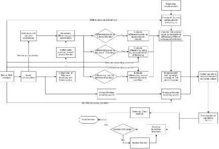
2.7 Development of System of Equations

A system of linear algebraic equations can now be developed to solve the governing

PDEs by combining the generalized cell-centred equations (2.20) or (2.22) and the nodal

value equations (2.24).

Suppose a mesh contains M triangular cells and N nodes (including interior and boundary

nodes). A system of N+M equations can be assembled and expressed in matrix form as:

(2.25)

where A is the coefficient matrix, is a column vector containing the constant values in

each equation (boundary values and rhs), and is a

variable vector containing all cell centroid and nodal values to be determined. The

column vectors of the coefficient matrix are linearly independent in N+M dimensional

space and therefore has a unique solution from the system of equations (2.25). Either a

(37)

22

2.8 Summary of CCFD Formulation

Sections 2.2 – 2.6 outline the derivation procedures for developing the system of

equations and the flow chart in Fig. 2.11 summarizes the development process.

Figure 2.11 Process of forming system of equations by CCFD scheme

The system of equations consists of equations for cell centroid values and equations for

nodal values. Cell centroid values are illustrated along the top branch in Fig. 2.11 and are

derived from finite difference approximations of the PDEs being solved. Nodal values are

shown along the bottom two branches with Dirichlet boundary points and the combined

set of interior and Neumann boundary points. The dependent variables at Dirichlet

boundary points are evaluated from the Dirichlet boundary conditions defined by the

PDE problem. In comparison, function values at the set of interior and Neumann

boundary points are determined by the length-weighted average of surrounding cell

centroid values. Once both cell centroid and nodal equations have been derived, the

system of equations is developed by formulating the coefficient matrix A and constant

column vector in the matrix form. The next chapter introduces a preliminary overview

(38)

23

CHAPTER 3 – PRELIMINARY OVERVIEW

3.1 Mesh Overview

Numerical methods based on the spatial subdivision of a domain into polyhedra imply the

need to generate a mesh. The mesh topology being studied in this thesis is based on a

triangulated domain created by Delaunay triangulation, which maximizes the minimum

angle of each triangle in the domain. Compared with the advancing front triangulation

technique, Delaunay triangulation generally yields a better quality mesh due to two main

reasons [4]:

1. Iteratively checks the discrepancy between the desired and actual element shape and

size of the current mesh.

2. Points are introduced into the regions where the discrepancy exceeds a user-defined

tolerance.

Delaunay triangulation in a plane ensures that the circumcircle associated with each

triangle contains no other mesh points in its interior domain [11]. Note that triangular

elements may create problems in structural loading applications, such as plane stress

problems. One problem is the geometric modeling of curved edges. The surface of a

model with a large curvature may appear reasonably modeled, whereas the surface of a

hole is poorly modeled. A second problem is that the strains in various regions of the

actual structure may be changing rapidly and the constant strain element will only

provide an approximation of the average strain at the centre of the element. For example,

loading in a nutshell will have poor approximation result when using triangular elements.

This problem can be solved either by increasing the number of elements (i.e. mesh

density), or alternatively replacing the triangular element with a better element, such as

an eight-noded quadrilateral [12].

3.1.1 Mesh Quality

The mesh quality can be evaluated with respect to two parameters: skewness and aspect

ratio. Skewness of a cell can be determined by the deviation from a normalized angle as

(39)

24

(3.1)

where is the normalized angle of a cell (i.e. 60o for

tetrahedral and triangular elements and 90o for quadrilateral and hexagonal elements).

Equation (3.1) implies that good cell quality results when skewness is close to 0 and bad

cell quality results when skewness is close to 1. For example, perfect cells with zero

skewness are equilateral triangles in a triangulated domain and rectangles in a

quadrilateral domain. As a general rule for acceptable mesh quality, skewness of

hexagonal, triangular and quadrilateral elements should not exceed 0.8.

Aspect ratio on the other hand is defined as the ratio of the longest side to the shortest

side of a mesh element. For an acceptable range of the aspect ratio, it should not be

greater than a value of 40, but the range can vary based on the characteristics of a

physical problem. By combining the effects of skewness and aspect ratio, the quality of a

triangle can be measured by the following equation [5]

(3.2)

where A is the triangle area and h1, h2 and h3 are the side lengths of the triangle. If q > 0.6,

the triangle is of acceptable quality. Note that an equilateral triangle has perfect quality

with q = 1 when h1 = h2 = h3.

3.1.2 Mesh Classification

Mesh types can be classified according to the following categories [4]:

1. Conformality

2. Surface or body alignment

3. Topology

4. Element Type

In principle, any of the four classifications can be combined randomly. However, only a

few main combinations are normally considered in the discretisation, which are as

(40)

25

a) Multiblock grids: Conformal, surface-aligned, macro-unstructured and

micro-structured grids consisting of quadrilaterals or bricks.

b) Adaptive Cartesian grids: Non-conformal, non-surface-aligned,

micro-unstructured grids consisting of quadrilaterals or bricks.

c) Unstructured uniform-element grids: Conformal, surface-aligned,

micro-unstructured grids consisting of triangles or tetrahedra.

In this thesis, an unstructured uniform-element mesh is implemented in solving physical

problems by the Cell-Centred Finite Difference scheme and other types of numerical

methodologies.

3.1.2.1 Conformality

Conformal meshes are characterized by continuous neighbouring elements across all

edges and faces [4]. Non-conforming meshes exhibit edges and faces that do not match

perfectly between neighbouring elements, which results in hanging nodes or overlapped

zones, as illustrated in Fig. 3.1.

Figure 3.1 Non-conformal mesh

Note in Fig. 3.1, that node A is a hanging node and face F1 becomes an overlapped zone

since the quadrilateral element does not match with the triangular elements at node A.

3.1.2.2 Surface or Body Alignment

Surface or body alignment refers to boundary faces matching exactly with grid points in

the surface domain [4]. If faces are crossed by the surface, the mesh is referred to as

being aligned. The following figures illustrated examples of surface aligned and

(41)

26

Figure 3.2 Examples of surface aligned and non-surface aligned meshes

Note that edges crossing the curve γ will create a node in the surface aligned mesh, but

not in the non-surface aligned mesh.

3.1.2.3 Mesh Topology

Mesh topology refers to the structure or order of the elements [4]. Three types of mesh

topology are:

1. Micro-structured: each interior node has the same number of neighbours.

2. Micro-unstructured: each interior node may have a different number of

neighbours.

3. Macro-unstructured, micro-structured: also refer as a staggered grid system. Mesh

is assembled from groups of micro-structured subgrids.

The following figure shows the three types of mesh topology.

Figure 3.3 Micro-structured, micro-unstructured and macro-unstructured, micro-structured meshes

Note that each interior node in the micro-structured mesh at the left of Fig. 3.3 has six

neighbouring cells and degrees. Interior nodes in the micro-unstructured mesh in the

middle figure have an arbitrary number of neighbouring cells and degrees. The figure on