Development of a Shape Memory Alloy Actuated Robotic Catheter for Endocardial Ablation: Modeling, Design Optimization, and Control.

(1)

ABSTRACT

CREWS, JOHN HUNTER. Development of a Shape Memory Alloy Actuated Robotic Catheter for Endocardial Ablation: Modeling, Design Optimization, and Control. (Under the direction of Dr. Gregory Buckner).

Atrial fibrillation is the most common cardiac arrhythmia, afflicting more than 2

million Americans. Symptoms include shortness of breath, fatigue, chest pain, stroke, and

even death. Treatment options consist of pharmacological, surgical, and electrophysiological

(ablation catheter-based) approaches. The ideal treatment would combine the effectiveness of

surgical methods with the minimally invasive attributes of catheter-based approaches.

However, commercially available catheters possess a number of limitations that hinder their

effectiveness. This dissertation focuses on the design optimization and control of a robotic

ablation catheter, internally actuated using shape memory alloys (SMAs), that overcomes

many of the limitations of existing ablation catheters.

The robotic ablation catheter is constructed from serially connected bending segments

actuated by internal SMA tendons. Each bending segment contains four SMA actuators that

contract upon heating and produce bending moments. The multiple actuators and segments

provide greater navigability for the physician. Coupled with the catheter’s

computer-controlled capabilities, this robotic catheter has the potential to improve success rates and

reduce procedure times in the treatment of AF, while simultaneously reducing healthcare

costs and radiation exposure to patients and medical staff.

The kinematics and inverse kinematics of the robotic catheter are developed in two

coordinate systems: three-dimensional Cartesian coordinates and generalized coordinates

(2)

2

generalized coordinates, while catheter tip measurements are made in Cartesian coordinates,

motivating the need for transformations between the two.

The catheter’s bending mechanics are described using a circular arc model, while

SMA actuation is modeled using free energy techniques. Two specific cases are considered:

single-tendon SMA actuation and antagonistic SMA actuation. Both cases are modeled using

COMSOL Multiphysics Modeling and Simulation Software and are experimentally

validated.

Design optimization of the robotic catheter is accomplished using the COMSOL

models and genetic algorithms (GAs). The geometry and material properties of each model

are parameterized and used as design variables in the GA. Both single-objective and

multi-objective cases are considered. The single-multi-objective problem optimizes the catheter’s radius

of curvature, a measure of its navigability. The multi-objective problem optimizes radius of

curvature and “pushability”, a quality related to catheter stiffness.

The computationally efficient hysteretic recurrent neural network (HRNN) is

implemented into a sliding mode control algorithm for the position control of SMA actuators.

The method is derived for a constant stress SMA actuator and demonstrated experimentally.

The control algorithm is extended to variable stress SMA actuators, the situation encountered

in the robotic catheter. Simulation results are presented for a single SMA actuator, and the

(3)

Development of a Shape Memory Alloy Actuated Robotic Catheter for Endocardial Ablation: Modeling, Design Optimization,

and Control

by

John Hunter Crews

A dissertation submitted to the Graduate Faculty of North Carolina State University

in partial fulfillment of the requirements for the degree of

Doctor of Philosophy

Mechanical Engineering

Raleigh, North Carolina

2011

APPROVED BY:

_______________________________ ______________________________

Gregory D. Buckner Paul I. Ro

Committee Chair

(4)

ii

DEDICATION

(5)

iii

BIOGRAPHY

John Crews was born and raised in Lexington, VA, where the only thing to do was

run. He came to North Carolina State University as an undergraduate to continue running. He

met his wife Amy at NCSU, who also ran for the cross country and track and field teams.

After receiving his B.S. in Mechanical Engineering in 2007, John interned in the summer at

the Johns Hopkins University Applied Physics Lab, where he realized (belatedly) that he

wanted to be a computer science major. In the fall of 2007, John began his doctoral degree in

Mechanical Engineering under the direction of Dr. Gregory Buckner. He continues to run,

(6)

iv

ACKNOWLEDGMENTS

I would like to thank Dr. Gregory Buckner for giving me with the opportunity and

freedom to pursue my interests. He supported me throughout the process, allowed me to

teach a class, and always pushed me to be my best. If I ever become a professor, it will

largely be due to his guidance and the insistence that he has the best job in the world.

I would like to thank my doctoral committee members: Dr. Scott Ferguson, Dr. Paul

Ro, and Dr. Ralph Smith. I truly have the best committee (maybe second to Jennifer

Hannen’s committee) and appreciate everyone’s guidance. Not only are they outstanding

committee members but also outstanding teachers, and their classes heavily influenced my

research and my career.

I thank all members of the Electromechanics Research Lab: J.P. Lien, Jennifer

Hannen, Qiaoyin Yang, Michael Mattson, and especially Shaphan Jernigan, Brian Owen, and

Andy Richards, who have helped me along the way. I am deeply indebted to Brian Owen,

who has bailed me out more times than I like to admit and never once complained when I

asked for a diagram. I am also sincerely grateful to Arun Veeramani, who was the ideal role

model early in my graduate career and showed me what hard work really is.

Above all I would like to thank my parents and my brothers, who always supported

me whenever I had a (supposedly) great idea. My parents pushed me to pursue what I love

and provided guidance along the way. My older brother Charlie never complained about

(7)

v

LIST OF TABLES

Table 3.1 SMA constitutive model parameters for the single-crystal model ... 54

Table 3.2 SMA constitutive model parameters for the polycrystalline model ... 56

Table 3.3 Single-tendon actuator model sensitivity to pre-strain ... 69

Table 3.4 Default values for single-tendon model perturbation ... 70

Table 3.5 Antagonistic actuation Model sensitivity to pre-strain ... 88

Table 3.6 Default values for antagonistic model perturbation ... 93

Table 4.1 Design variables and bounds ... 114

Table 4.2 Optimal design variables and objective function for the single-objective optimization of a single tendon ... 116

Table 4.3 Optimal design variables and objective function for the single-objective optimization of a single tendon ... 119

Table 4.4 Optimal design variables and objective function for the single-objective optimization of a antagonistic actuation ... 122

Table 4.5 Optimal design variables and objective functions for the multi-objective optimization of antagonistic actuation ... 124

(13)

xi

LIST OF FIGURES

Figure 1.1 Electrical differences in heart with normal sinus rhythm (a) and heart with atrial

fibrillation (b) [2]... 1

Figure 1.2 Incisions and excisions for Cox Maze I [8] ... 2

Figure 1.3 Lesions created using multiple discrete ablation points (shown in red) [13] ... 3

Figure 1.4 Conventional steerable ablation catheter: (a) catheter tip and handle; (b) planar bending ... 5

Figure 1.5 Commercially available robotic catheter systems: (a) Niobe II [15]; (b) Sensei system [16] ... 6

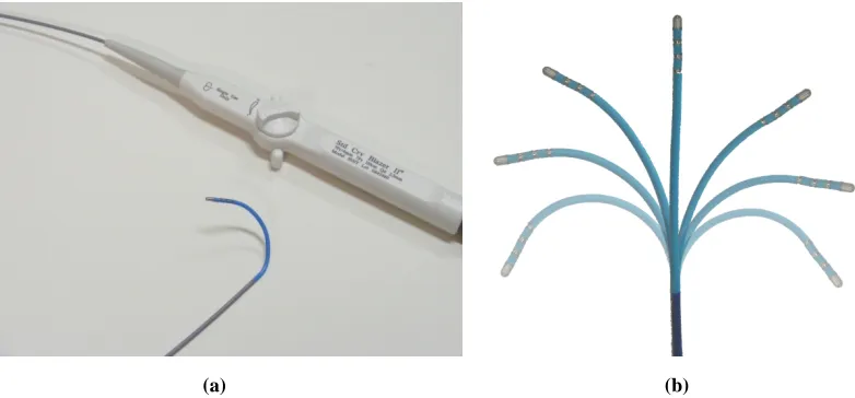
Figure 1.6 Robotic catheter prototype: (a) schematic; (b) photograph; (c) laser cut SMA actuator ... 7

Figure 1.7 Electrophysiology lab with robotic catheter system installed ... 8

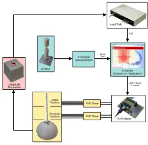
Figure 1.8 Robotic catheter system components ... 9

Figure 2.1 Robotic catheters: (a) single bending segment; (b) two bending segments ... 16

Figure 2.2 Generalized coordinates for robotic catheter ... 17

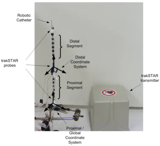
Figure 2.3 Vertical coordinate system for a catheter with multiple segments ... 18

Figure 2.4 Time-lapsed photography of the catheter bending with circular arc references [19] ... 19

Figure 2.5 Geometry for catheter bending less than 90o ... 20

Figure 2.6 Geometry for catheter bending greater than 90o ... 22

Figure 2.7 Simulation of catheter motion: fixed distal segment (90o) and rotating proximal segment ... 26

(14)

xii

Figure 2.9 Two-segment catheter with coordinate systems and rotation ... 29

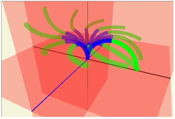
Figure 2.10 Multiple catheter solutions that reach a given 3D tip location ... 33

Figure 2.11 Flowchart for conjugate gradient algorithm ... 34

Figure 2.12 CG results for a reference distal location: (a) cost; (b) resulting geometry... 35

Figure 2.13 GA results for a reference distal location: (a) cost; (b) resulting geometry ... 37

Figure 2.14 Desired distal location and direction: (a) general case of a catheter located in the left atrium; (b) simplified case for the vertical catheter setup ... 38

Figure 2.15 CG results for a reference distal location and normal: (a) cost; (b) resulting geometry ... 41

Figure 2.16 GA results for a reference distal location and normal: (a) cost; (b) resulting geometry ... 42

Figure 3.1 Flexible beam actuated by SMA: (a) single actuator case; (b) antagonistic actuator case ... 44

Figure 3.2 Thermo-mechanical coupling of SMA crystalline phases ... 46

Figure 3.3 Stress-strain response of a SMA actuator attached to a flexible beam ... 47

Figure 3.4 Effects of the SMA model parameters that govern the phase fraction transition probabilities ... 49

Figure 3.5 Stress-strain validation for a the single-crystal model: (a) 24 oC; (b) 45 oC; (c) 75 o C; (d) 95 oC ... 55

Figure 3.6 Stress-strain validation for a the polycrystalline model (N=5): (a) 24 oC; (b) 45 oC; (c) 75 oC; (d) 95 oC ... 57

Figure 3.7 Stress-strain validation for a the polycrystalline model (N=25): (a) 24 oC; (b) 45 o C; (c) 75 oC; (d) 95 oC ... 58

Figure 3.8 Stress-strain validation for a the polycrystalline model (N=50): (a) 24 oC; (b) 45 o C; (c) 75 oC; (d) 95 oC ... 59

(15)

xiii

Figure 3.10 Experimental test rig for bending model validation: (a) photograph of the entire setup; (b) illustration of the collets showing slots to control actuator offset from the neutral axis ... 65

Figure 3.11 Comparison between the radius of curvature for the single-crystal model, polycrystalline model, and the experimental data for four actuator offsets: (a) 0.67 mm; (b) 1.05 mm; (c) 1.42 mm; (d) 1.92 mm ... 66

Figure 3.12 Comparison between the radius of curvature for the single-crystal model, polycrystalline model, and the experimental data for four pre-strains: (a) 4.0 %; (b) 4.5 %; (c) 5.0 %; (d) 5.5 % ... 68

Figure 3.13 Simulated bending model dependence on the elastic modulus of the beam: (a) radius of curvature; (b) stress-strain response... 71

Figure 3.14 Simulated bending model dependence on the radius of the beam: (a) radius of curvature; (b) stress-strain response ... 72

Figure 3.15 Simulated bending model dependence on the radius of the SMA actuator: (a) radius of curvature; (b) stress-strain response... 73

Figure 3.16 Simulated bending model dependence on the offset from the neutral axis: (a) radius of curvature; (b) stress-strain response... 73

Figure 3.17 Simulated bending model dependence on the pre-strain: (a) radius of curvature; (b) stress-strain response ... 75

Figure 3.18 Simulated bending model dependence on the thermal boundary condition: (a) radius of curvature; (b) stress-strain response; (c) final temperature distribution; (d) final distribution of austenite phase fraction ... 76

Figure 3.19 Three-dimensional bending decoupled into two planar bending problems ... 78

Figure 3.20 Simplified one-dimensional system for a flexible beam actuated by antagonistic SMA tendons ... 79

Figure 3.21 One-dimensional COMSOL model for antagonistic actuation ... 80

Figure 3.22 Antagonistic experimental test rig: (a) photograph; (b) schematic of the four different collets ... 83

(16)

xiv

Figure 3.24 Comparison between the radius of curvature for the single-crystal model, polycrystalline model, and the experimental data for four actuator offsets: (a) 0.8 mm; (b) 1.05 mm; (c) 1.42 mm; (d) 1.92 mm ... 85

Figure 3.25 Close-up of the radius of curvature for two offsets: (a) 1.42 mm; (b) 1.92 mm . 86

Figure 3.26 Comparison between the radius of curvature for the single-crystal model, polycrystalline model, and the experimental data for four pre-strains: (a) 2.3%; (b) 2.74%; (c) 3.62%; (d) 4.06% ... 87

Figure 3.27 Results of the Monte Carlo analysis: (a) distribution of pre-strain corresponding to one turn (0.45%); (b) distribution of pre-strain corresponding to 11 turns (5.0%); (c) distribution of radius of curvature for one turn (0.45% pre-strain); (d) distribution of radius of curvature for 11 turns (5.0% pre-strain) ... 91

Figure 3.28 Comparison between 95% confidence intervals predicted from Monte Carlo analysis and experimental data for two offset distances: (a) 1.05 mm; (b) 1.42 mm ... 92

Figure 3.29 Simulated bending model dependence on the elastic modulus of the beam: (a) radius of curvature; (b) strain response for the active actuator; (c) stress-strain response for the inactive actuator ... 94

Figure 3.30 Simulated bending model dependence on the radius of the beam: (a) radius of curvature; (b) stress-strain response for the active actuator; (c) stress-strain response for the inactive actuator ... 96

Figure 3.31 Simulated bending model dependence on the radius of the SMA actuator: (a) radius of curvature; (b) strain response for the active actuator; (c) stress-strain response for the inactive actuator ... 97

Figure 3.32 Simulated bending model dependence on the offset from the neutral axis: (a) radius of curvature; (b) strain response for the active actuator; (c) stress-strain response for the inactive actuator ... 98

Figure 3.33 Simulated bending model dependence on the pre-strain: (a) radius of curvature; (b) stress-strain response for the active actuator; (c) stress-strain response for the inactive actuator ... 100

(17)

xv

Figure 4.1 General flow chart of a GA... 109

Figure 4.2 Flow chart for single-objective GA ... 111

Figure 4.3 GA results for the single-objective optimization of a single SMA actuator: (a) average fitness of the population; (b) fitness of the best individual in the population ... 115

Figure 4.4. MOGA results for the single SMA actuator: (a) population number vs. generation; (b) evolution of the Pareto frontier; (c) final Pareto frontier ... 118

Figure 4.5 GA results for the single-objective optimization of antagonistic SMA actuation: (a) average fitness of the population; (b) fitness of the best individual in the population ... 121

Figure 4.6 MOGA results for antagonistic SMA actuation: (a) population number vs. generation; (b) evolution of the Pareto frontier; (c) final Pareto frontier ... 123

Figure 5.2 HRNN architecture ... 133

Figure 5.3 SMA tendon actuating a suspended mass ... 137

Figure 5.4 Constant-stress SMA tendon ... 138

Figure 5.5 Monotonicity of reference temperature: only one reference temperature achieves the desired displacement ... 141

Figure 5.6 Overview of control scheme ... 142

Figure 5.7 SMC for constant-stress SMA actuator ... 144

Figure 5.8 Experimental setup for measuring SMA hysteresis: (a) photograph; (b) schematic ... 145

Figure 5.9 Experimental training data acquired from the SMA test rig: (a) input current; (b) SMA surface temperature; (c) SMA displacement ... 146

Figure 5.10 Evolution of the augmented cost function and the error cost function ... 148

(18)

xvi

Figure 5.12 Simulation results for the SMC: (a) displacement; (b) input current; (c)

temperature ... 150

Figure 5.13 Close-up of the simulated response of the SMA actuator: (a) displacement; (b) temperature ... 151

Figure 5.14 Experimental tracking results for the constant-stress SMA actuator ... 152

Figure 5.15 Experimental input current for the constant-stress SMA actuator ... 153

Figure 5.16 Single SMA tendon attached to a flexible beam ... 154

Figure 5.17 Comparison of hysteresis plots for simulated data and HRNN prediction: (a) input current; (b) temperature; (c) recovered strain for constant-stress case; (d) recovered strain for variable-stress case ... 155

Figure 5.18 SMC for variable-stress SMA actuator ... 157

Figure 5.19 Simulated variable-stress data for HRNN training: (a) input current; (b) temperature; (c) bending angle... 158

Figure 5.20 Evolution of the augmented cost function and the error cost function ... 159

Figure 5.21 Comparison of hysteresis plots for simulated data and HRNN prediction: (a) ascending transitions; (b) descending transitions ... 160

Figure 5.22 Simulated response for the SMC: (a) bending angle; (b) input current ... 161

Figure 5.23 Comparison between the PID and SMC: (a) bending angle; (b) input current.. 162

Figure 5.24 Antagonistic SMA tendons attached to a flexible beam ... 163

Figure 5.25 Comparison between trained HRNN and experimental data for antagonistic SMA actuators ... 164

Figure 6.1 Cross section of a manually actuated catheter ... 168

Figure 6.2 Extending the SMA tendon length beyond the active segment of the catheter: (a) current prototypes where the SMA length is the constrained to the bending segment; (b) example of prototype with SMA tendons than extend into the rigid segment; (c) another example of longer SMA tendon ... 169

(19)

1

Chapter 1. Introduction

1.1 Motivation

Atrial fibrillation (AF) is the most common cardiac arrhythmia, afflicting over 2.2

million Americans with 160,000 new cases diagnosed each year [1]. The disease is

associated with shortness of breath, fatigue, chest pain, stroke, and even death. AF is

characterized by random electrical impulses in the atria, disrupting the heart’s normal

rhythm. The electrical pathways associated with normal sinus rhythm and atrial fibrillation

are shown in Figure 1.1.

(a) (b)

(20)

2

Treatment options for atrial fibrillation include pharmacological, surgical, and

electrophysiological approaches. Pharmacological approaches are usually the first choice of

treatment, but are frequently ineffective [3] or cause significant side effects [4]. Surgical

approaches are often highly invasive, requiring “open-chest” access and cardiopulmonary

bypass. The most popular treatment for AF was developed by James Cox [5]. Known as the

“Cox Maze” procedure, it involves multiple incisions through atrial tissue to block the

conduction of electrical signals (Figure 1.2). Refinements to the original Cox Maze

procedure (Cox Maze II and III) have made it the gold standard for treating AF [6], with

success rates as high as 96% [7].

(21)

3

Electrophysiological treatments for AF are performed with cardiac ablation catheters,

requiring only small incisions to gain peripheral vascular access. However, the efficacy of

catheter-based treatments varies widely, with an average success rate of only 52% [9].

Catheter-based approaches involve ablating atrial tissue to block electrical sources and

pathways, often near the pulmonary veins [10]. The catheter tip uses either radiofrequency

(RF) alternating currents or cryogenic agents to create lesions through the atrial wall.

Depending on the patient-specific physiology, the ablation process either targets specific

points (ectopic foci), creates linear lesions, or both. Effective lesion sets mimic those

specified in the Cox Maze procedure and must be both transmural (completely penetrating

the atrial tissue) and continuous. However, linear lesions are created using a point-by-point

method, Figure 1.3, often resulting in gaps that decrease the procedural efficacy [11].

Furthermore, this point-by-point method results in long procedure times (179 min average)

[12], exposing both the patient and medical staff to long durations of fluoroscopy.

(22)

4

The ideal treatment for AF would combine the minimally invasive attributes of

catheter-based approaches with the effectiveness of surgical approaches [14]. Such a

treatment can be realized via computer-assisted catheter manipulation [10]. By improving

navigability and utilizing a computer-controlled approach, the ablation catheter would be

better suited to reach difficult locations and create continuous, linear lesions. The result

would be improved success rates, reduced procedure times, and reduced exposure to

fluoroscopy for both the patient and the medical staff.

1.2 Commercial ablation catheters

Commercially available RF ablation catheters are manually steerable in a

bi-directional sense, as shown in Figure 1.4. These catheters are capable of tracing arcs in a

single plane. Their limited degrees of freedom require electrophysiologists to spend

significant time manually advancing, rotating, and bending the catheter tip to access the

target anatomy. Furthermore, continuous linear lesions are nearly impossible to achieve using

manually actuated catheters.

(23)

5

(a) (b)

Figure 1.4 Conventional steerable ablation catheter: (a) catheter tip and handle; (b) planar bending

Two robotic catheter systems are commercially available. The Niobe Magnetic

Navigation System from Sterotaxis (St. Louis, MO) uses two external permanent magnets to

control the catheter tip, Figure 1.5a. The primary disadvantages of the Niobe system are that

it requires significant capital investments and extensive modifications to the catheter lab. The

Sensei Robotic Catheter System from Hansen Medical (Mountain View, CA) uses pull-wires

attached to external motors to deflect the catheter tip. The system consists of a large diameter

sheath (14 Fr) with two degrees of freedom and a single controllable segment on the ablation

catheter, Figure 1.5b. The disadvantages of the Sensei system are its large diameter (making

it unsuitable for pediatric cases) and the additional space needed to externally actuate the

(24)

6

(a) (b)

Figure 1.5 Commercially available robotic catheter systems: (a) Niobe II [15]; (b) Sensei system [16]

1.3 Overview of the SMA actuated robotic catheter

Our robotic catheter uses shape memory alloys (SMAs) for internal actuation. SMAs

are novel “smart materials” capable of recovering large strains upon heating. This shape

memory effect makes them ideally suited for actuation applications requiring large energy

densities. Furthermore, their biocompatibility is well-suited to in-vivo actuation applications

like endocardial ablation.

The bending segments of our robotic catheter prototype feature three main

components: SMA actuators (tendons), an axially stiff, laterally compliant central structure,

and collets (Figure 1.6). The SMA tendons are either wires (FLEXINOL actuator wires from

Dynalloy Inc., Tustin, CA) or custom laser cut strips (fabricated by Memry GmbH, Weil am

Rhein, Germany) as shown in Figure 1.6c. The collets hold the SMA actuators a fixed

distance from the neutral axis of the central structure (beam), creating a moment as the

(25)

7

can vary considerably; hence, one goal of this dissertation is to determine optimal

configurations.

(a) (b)

(c)

Figure 1.6 Robotic catheter prototype: (a) schematic; (b) photograph; (c) laser cut SMA actuator

The robotic catheter system has a number of potentially significant advantages,

(26)

8

Additionally, the robotic catheter does not significantly alter the equipment or procedures of

conventional catheter labs. Whereas the Niobe and Sensei systems both remove the

electrophysiologist from the patient’s bedside, our robotic catheter system will be utilized in

a manner similar to conventional (manually-actuated) ablation procedures (Figure 1.7). The

forward motion of the catheter will still be controlled manually, providing tactile feedback to

the operator and reducing the risk of tissue perforations.

Figure 1.7 Electrophysiology lab with robotic catheter system installed

A schematic of the robotic catheter system components is shown in Figure 1.8. The

(27)

9

dissipated power (and internal temperature) of each SMA tendon. A master-slave AVR

system determines the PWM percentages for each tendon and modulates the currents by

switching MOSFETs. For precise control of the catheter, accurate position measurements are

necessary. Currently, a trakSTAR 3D Magnetic Tracking System (Ascension Technology

Corporation, Burlington, VT) is used for this purpose. The trakSTAR system can

simultaneously monitor the 3D locations and orientations of up to four points on the catheter.

A joystick provides the tracking reference for navigation purposes. Finally, a custom C++

application ties together all of the sensors and actuators and provides a platform for real-time

control.

(28)

10

Operationally, the robotic catheter system is capable of set-point regulation or

closed-loop tracking of a joystick reference or pre-determined reference path. These operational

modes correspond to specific situations encountered in catheter ablation of AF. When a

specific point needs to be ablated, the computer-controlled robotic catheter will navigate to

that location. Closed-loop tracking of a joystick reference will be used for general navigation

and when the electrophysiologist wants direct control of the catheter. Closed-loop tracking of

a reference path will be necessary to create continuous lesions based on a subset of points

specified by the electrophysiologist.

1.4 Prior Work

The development of our robotic catheter utilizes and extends previous research

involving the modeling, optimization, and control of SMAs. An overview of this prior work

is presented next.

1.4.1 Modeling and control of SMAs

Shape memory alloys are unique materials with properties that exhibit nonlinear,

hysteretic dependence on stress and temperature. Because of their high energy densities,

impressive strain recovery characteristics, and biocompatibility, they have the potential to

revolutionize robotic actuation in biomedical applications. SMAs exhibit two unique and

useful characteristics: the super-elastic effect and the shape memory effect. To date,

biomedical applications have largely utilized the super-elastic properties of SMAs [17];

(29)

11

[18]. By contrast, most biomedical technologies utilizing the shape memory effect are still in

the research and development phases. This shape memory effect, which allows SMAs to

contract by over 4% upon heating, is currently being incorporated into cardiac catheters [19],

annuloplasty bands [20], and smart inhaler systems for aerosol drug delivery [21].

The precise control of SMA actuators is complicated by rate-dependent, hysteretic

dependencies of strain, stress and temperature. To address these technical challenges, both

model-based and heuristic control algorithms have been developed. Model based control

algorithms utilize both physical models [22] and empirical models [23]. Other approaches

have relied on neural networks to compensate for hysteresis [24]. Heuristic approaches such

as proportional-integral-derivative (PID) control have also been demonstrated [25].

1.4.2 Optimization of SMAs

While the published research has focused primarily on specific modeling and control

aspects of SMAs, little attention has been paid to the design optimization of SMA-actuated

systems. The design of SMA actuators is often iterative and non-intuitive due to the

material’s complex thermo-mechanical behavior. The limited work on SMA design

optimization has either focused on the material’s super-elastic behavior [26] or is based on

empirical models [27], [28]. In [26], the authors investigate the optimal hysteresis loop

shapes for SMA’s use as an energy dissipation device, which requires modifying the

(30)

12

In [27], the authors optimize the weight of a corrugated plate actuated by SMA

subject to certain performance constraints. In [28], the authors use an exponential empirical

model [30] within a finite element model for optimization of SMA spring actuators for

endoscopes. The geometry of the springs is optimized, but the authors fail to fully quantify

the actuator’s capabilities.

1.5 Research objectives

The research summarized in this dissertation advances the development of a robotic

RF ablation catheter by optimizing the design of shape memory alloy actuated structures. The

goal is to enhance specific performance metrics through optimization of critical design

variables. Additionally, new control schemes are developed to address inherent nonlinearities

and enable the use of SMA as an actuator in precision control applications. This optimized

catheter has the potential to revolutionize the treatment of AF and other therapies (i.e.

brachytherapy for the treatment of cancer [31]). Furthermore, the design optimization and

control methods presented here are applicable to a wide range of applications involving

SMA-actuated flexible structures.

The specific aims are:

• Develop the kinematics for single-segment and multi-segment robotic catheters in

(31)

13

• Develop and validate finite element models of flexible beams actuated by SMAs for

single actuators and antagonistic actuators.

• Present methods for optimizing SMA actuated flexible beams such as the robotic

ablation catheter.

• Develop control algorithms that compensate for the hysteresis inherent in SMA

actuators.

1.6 Dissertation outline

This dissertation is organized as follows:

Chapter 2: Flexible Catheter Kinematics

This chapter provides the framework for transforming the locations of catheter segments

between two coordinate systems. Modeling the catheter’s kinematics is important for

navigation and control purposes. As will be shown, the easiest way to describe the catheter

kinematics is in terms of bending angles; however, experimental position measurements are

normally made in Cartesian coordinates. Being able to efficiently transform between the two

coordinate systems is critical for real-time control. Furthermore, it is necessary to understand

the workspace of the robotic catheter for surgical navigation and ablation purposes. This

chapter develops the transformations between the two coordinate systems for a

single-segment and a two-single-segment catheter. Additionally, the inverse kinematics and solutions are

(32)

14

Chapter 3: Finite Element Modeling of SMA Actuated Flexible Beams

This chapter develops the SMA constitutive model and bending mechanics for robotic

ablation catheters actuated by single SMA tendons and antagonistic SMA tendons. Accurate

models are essential to predicting the performance of robotic catheter designs. Veeramani

originally developed a single-crystal model of the robotic catheter [19]; here, the model is

incorporated into COMSOL Multiphysics Modeling and Simulation Software (COMSOL

Inc., Burlington, MA), a finite element software package. The bending model is simplified to

a one-dimensional problem that is validated experimentally. Additionally, a polycrystalline

model is implemented for the first time in COMSOL and experimentally validated.

Perturbation and sensitivity analyses are also presented.

Chapter 4: Design Optimization of the Robotic Catheter

The optimization of nonlinear, hysteretic materials such as SMAs is complex and

non-intuitive. By combining accurate, experimentally validated models with efficient

optimization algorithms, a simulation-based design strategy can be employed to reduce the

time spent on prototyping and experimentally evaluating iterative design concepts.

This chapter presents design optimization methods for the robotic catheter, including

single-objective and multi-objective optimization for single and antagonistic actuators. For

the single-objective optimization, the objective function to be minimized is the catheter’s

(33)

15

catheter’s radius of curvature and “pushability”. The optimal designs are found using genetic

algorithms.

Chapter 5: Control of the Robotic Catheter

Precise, real-time control of the robotic ablation catheter is necessary for procedural

efficacy. The success of the robotic catheter will be dependent on its ability to accurately

ablate locations and create continuous lesions. Both procedures require real-time control

algorithms that effectively compensate for hysteresis and are computationally efficient.

This chapter presents methods for controlling a single SMA actuator using hysteretic

recurrent neural networks (HRNNs). The case of a single SMA actuator under constant stress

is considered. The HRNN is used as the inverse model to provide a reference temperature

given a reference displacement. A sliding mode controller is then used on the heat transfer

model to drive the actual temperature to the reference temperature. While the actuator is

under constant stress, the extension to SMA actuators attached to a flexible beam is presented

with simulation results.

Chapter 6: Conclusion

Chapter 6 provides the conclusions and discusses possible future work. Extensions of

(34)

16

Chapter 2. Flexible Catheter Kinematics

2.1 Introduction

This chapter develops the kinematics and coordinate transformations that are

necessary for real-time control of a robotic ablation catheter. Two different systems are

considered: a single-segment catheter (Figure 2.1a) and a two-segment catheter (Figure 2.1b).

Cases involving more than two segments are simply extensions of the two-segment case.

(a) (b)

(35)

17

For robotic systems possessing multiple degrees of freedom (like the robotic ablation

catheter of Figure 1.6), it is important to succinctly describe the system kinematics.

Commercial measurement platforms such as the trakSTAR 3-D guidance system (Ascension

Technology Corp, Burlington, VT) are capable of real-time position monitoring in

three-dimensional Cartesian coordinates. For the robotic catheter, however, it is easier to design

and implement control algorithms using generalized bending coordinates (bending angle θ and orientation angle ϕ, Figure 2.2) for each catheter segment (since each possesses only two degrees of freedom). This chapter develops the transformations between the two

coordinate systems for a single-segment and a two-segment catheter. Additionally, the

inverse kinematics and solutions are presented.

(36)

18

When navigating a catheter within a human body, multiple coordinate systems are

necessary, including the moving coordinate systems (or frames) attached to each catheter

segment and the global (or fixed, inertial) coordinate system. To simplify the subsequent

derivations, a vertical setup for the robotic catheter is considered (Figure 2.3), where the

proximal and global coordinate systems are the same because the base of the catheter is

fixed.

Figure 2.3 Vertical coordinate system for a catheter with multiple segments

A single segment robotic catheter was originally designed and modeled by Veeramani

[19], [32]. He found that the catheter follows a circular arc bending model, Figure 2.4. In [3],

Ganji, et. al modeled the kinematics of a manually actuated, bi-directional catheter with a

(37)

19

experimental results, the authors in [3] validated the accuracy of the circular arc model and

the zero torsion (planar bending) assumption.

Figure 2.4 Time-lapsed photography of the catheter bending with circular arc references [19]

2.2 Coordinate transformations for a single-segment catheter

In this section, the coordinate transformations for a single-segment robotic catheter

are derived. These transformations will also be necessary for describing the geometry of

multi-segment robotic catheters. In Section 2.2.1, the transformation from experimental

measurements (in 3D Cartesian coordinates) to generalized coordinates is derived. This

transformation is important because control algorithms will be concerned with tracking errors

in generalized coordinates. In Section 2.2.2, the transformation from generalized to Cartesian

(38)

20

2.2.1 Transformation from Cartesian to generalized coordinates

Two different cases must be considered when transforming from 3D Cartesian

coordinates to 2D generalized coordinates: bending angles θ less than 90o and bending angles greater than 90o. For the case of a bending angle less than 90o, the geometry presented in Figure 2.5 is utilized.

Figure 2.5 Geometry for catheter bending less than 90o

The rotation angle is defined to be

atan2 y

x ϕ =  _{ }

 . (2.1)

While the bending angle θ is simply

atan z

b θ =  _{ }

(39)

21 Furthermore,

a b+ =R, (2.3)

and

2 2

a= x +y . (2.4)

Combining the Euclidean norm

2 2 2

z +b =R , (2.5)

with (2.3) - (2.5) results in

(

)

2

2 2 2 2

z + R− x +y =R . (2.6)

Rearranging yields

2 2 2 2 2

2

x y z

R

x y

+ +

=

+ . (2.7)

Therefore,

(

)

2 2 2 2 2

atan atan 2 atan z b z R a

z x y

z x y

θ =  _{ }     = _ _ −    ₊    = _ _ − +  

. (2.8)

(40)

22

(a) (b)

Figure 2.6 Geometry for catheter bending greater than 90o

The rotation angle remains

atan2 y

x ϕ =  _{ }

 . (2.9)

Defining the supplementary angle

o

180

α = −θ , (2.10)

leads to

atan z

b α =  _{ }

 , (2.11)

and the following relationships:

2 2 2

x +y =a , (2.12)

R b+ =a, (2.13)

(41)

23

2 2 2

z +b =R . (2.14)

Combining (2.13) and (2.14) provides

2 2 2 a z b a a +

= − . (2.15)

Substituting (2.15) into (2.11) yields

2 2 atan 2 z a z a a α     =   +  ₋     

. (2.16)

And from (2.12)

2 2 2 2 2

2 2 2 2

2 2 2

atan

2

2 atan

z

x y z

x y

z x y

x y z

α       = _ _ + + + −    ₊     ₊    = _ _ + −  

. (2.17)

Finally, the bending angle can be expressed as

2 2 2 2 2

2

atan z x y

x y z

θ π= − _ + _

+ −

 

. (2.18)

In order to determine whether the bending angle is less than or greater than 90o, the following relationship is necessary. If the catheter is bending exactly 90o, then

2L z

π

(42)

24

where L is the length of the catheter. If the measured distance z 2L

π

≥ , then Equation (2.8) is

used to convert the measured (Cartesian) coordinates to generalized coordinates. If the

measured distance z 2L

π

< , then Equation (2.18) is used to convert the measured coordinates

to generalized coordinates. In summary, Equation (2.20) can be used to transform the

three-dimensional trakSTAR measurements to two-three-dimensional generalized coordinates.

(

)

2 2 2 2 2

atan2 2 2 atan if 2 2 atan if y x

z x y L

z

z x y

z x y L

z

x y z

ϕ π θ π π   = _{ }     ₊     ≥  − +     =   

 ₋ _ + _ _<

 _ ₊ ₋ _

  



. (2.20)

2.2.2 Transformation from generalized to Cartesian coordinates

Calculating Cartesian coordinates from the generalized coordinates is straightforward

for both cases. For the case of o

90

θ ≤ , from Figure 2.5 it is obvious that

( )

sin

z=R θ . (2.21)

Furthermore, note the arc length relationship

L=Rθ, (2.22)

where L is again the length of the catheter. Therefore, knowing the length of the catheter

(43)

25

( )

sin L z θ θ

= . (2.23)

It can also be shown that

( )

cos

x=a ϕ , (2.24)

and

( )

sin

y=a ϕ . (2.25)

Combining Equations (2.3) and (2.22) with the relationship

( )

cos

b=R θ , (2.26)

results in

( )

(

1 cos

)

cos

( )

L

x θ ϕ

θ

= − , (2.27)

and

( )

(

1 cos

)

sin

( )

L

y θ ϕ

θ

= − . (2.28)

For the case of o

90

θ > , the derivation is similar. The end result is:

(

)

sin

L

z π θ

π θ

= −

− , (2.29)

(

)

(

1 cos

)

cos

( )

L

x π θ ϕ

π θ

= − −

− , (2.30)

and

(

)

(

1 cos

)

sin

( )

L

y π θ ϕ

π θ

= − −

(44)

26

2.3 Coordinate transformations for a two-segment catheter

For a robotic catheter with multiple bending segments, the coordinate transformations

become more challenging. Figure 2.7 illustrates the motion of a 2-segment catheter with a

fixed distal segment (with respect to its own moving coordinate system) while the proximal

segment rotates. The combined motion of these segments is significantly different than that

of serial robotic manipulators, which rotate about 1 DOF revolute joints.

Figure 2.7 Simulation of catheter motion: fixed distal segment (90o) and rotating proximal segment

The inverse kinematics problem involves determining the proximal and distal angles

prox

θ , ϕ_prox, θ_dist, and ϕ_dist, given three simultaneous measurements: 0

[

0 0 0

]

T

x y z

=

p ,

[

]

1 1 1 1

T

x y z

=

p , and 2

[

2 2 2

]

T

x y z

=

p , corresponding to the Cartesian coordinates of the

(45)

27 following assumption is used: 0

[

0 0 0

]

T =

p . A schematic showing these measurements

and the generalized coordinates is provided in Figure 2.8.

Figure 2.8 Two-segment catheter showing measurement vectors and generalized coordinates

In general, three coordinate systems are required to represent a two-segment catheter:

the proximal coordinate system (denoted ˆx), the distal coordinate system (denoted x%), and

the global coordinate system (denoted x). However, for the simplified vertical catheter setup

shown in Figure 2.3, only the first two coordinate systems are necessary since the proximal

(46)

28

2.3.1 Transformation from generalized to Cartesian coordinates

Given a set of four generalized coordinates θprox, ϕprox, θdist, and ϕdist, the Cartesian

coordinates of the proximal tip can be found using either Equations (2.23), (2.27), and (2.28)

or Equations (2.29), (2.30), and (2.31). For example, if the bending angle of the proximal

segment is less than 90o as determined by (2.19), its Cartesian coordinates are

( )

1 sin prox prox

L

z θ

θ

= , (2.32)

( )

(

)

( )

1 1 cos prox cos prox

prox L

x θ ϕ

θ

= − , (2.33)

and

( )

(

)

( )

1 1 cos prox sin prox

prox L

y θ ϕ

θ

= − . (2.34)

Equations (2.32) - (2.34) are expressed in global coordinates since the global

coordinate system is the same as the proximal coordinate system. For the distal segment, the

tip coordinates are computed with respect to the distal coordinate system using either

Equations (2.23), (2.27), and (2.28) or Equations (2.29), (2.30), and (2.31). For example, if

the distal bending angle is also less than 90o as determined by (2.19), the tip coordinates are

( )

2 sin dist dist

L

z θ

θ

=

% , (2.35)

( )

(

)

( )

2 1 cos dist cos dist

dist L

x θ ϕ

θ

= −

(47)

29 and

( )

(

)

( )

2 1 cos dist sin dist

dist L

y θ ϕ

θ

= −

% . (2.37)

These distal tip coordinates can be transformed to the global coordinate system (also

the proximal coordinate system for the simplified vertical catheter setup). A schematic of the

coordinate systems and associated rotations is provided in Figure 2.9.

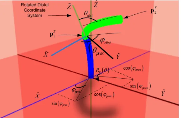
Figure 2.9 Two-segment catheter with coordinate systems and rotation

The normalized location of the proximal segment in the X −Y plane is

( )

1 cos sin 0

T

prox prox

ϕ ϕ

 

=  

u . To transform the distal coordinates to the global

(48)

30

( )

(

( )

)

( )

( ) ( )

(

( )

)

( ) ( )

(

( )

)

( )

(

( )

)

( ) ( ) ( )

( ) ( )

( )

2 2

s 1 c c s c 1 c c s

s c 1 c c 1 c c s s

c s s s c

prox

prox prox prox prox prox prox prox prox prox prox prox prox prox prox prox prox

prox prox prox prox prox

θ ϕ θ θ ϕ ϕ θ ϕ θ ϕ ϕ θ ϕ θ θ ϕ θ ϕ θ ϕ θ θ =  ₋ ₊ ₋ ₋    ₋ ₋ ₋ ₊     ₋ ₋      u R . (2.38)

In (2.38), c

( )

refers to cos

( )

, and s

( )

refers to sin

( )

. Using the above matrix,

the Cartesian coordinates in the distal coordinate system ( 2

[

2 2 2

]

T

x y z

=

p% % % % ) can be

transformed to the global coordinate system

( )

2 = +1 u θprox 2

p p R p% , (2.39)

where 2

[

2 2 2

]

T

x y z

=

p and 1

[

1 1 1

]

T

x y z

=

p .

2.3.2 Transformation from Cartesian to generalized coordinates

Since measurements are made in Cartesian coordinates using the trakSTAR system,

the reverse transformation (from Cartesian to generalized coordinates) is important. Given a

pair of measurements p₁T =

[

x₁ y₁ z₁

]

and pT₂ =

[

x₂ y₂ z₂

]

and assuming

[

]

0 0 0 0

T =

p , the proximal angles can immediately be found from either Equations (2.1)

and (2.8) or Equations (2.9) and (2.18). For example, if the proximal tip angle is less than

90o, the angles are

1 1 atan2 prox y x ϕ =  _{ }

(49)

31 and

(

)

2 2 1 1 1 2 2 2 1 1 1

2 atan

prox

z x y

θ = _ + _

− +

 

. (2.41)

The distal measurement is then transformed to its own coordinate system,

[

]

( )

1

(

)

2 x2 y2 z2 θprox 2 1

−

= = u +

p% % % % R p p . (2.42)

Finally, the angles are found from either Equations (2.1) and (2.8) or Equations (2.9)

and (2.18). For example, if the distal tip angle is less than 90o, the angles are

2 2 atan2 dist y x ϕ = _ _

 , (2.43)

and

(

)

2 2 2 2 2 2 2 2 2 2 2

2 atan

dist

z x y

θ = _ + _ − +   % % % % %

% . (2.44)

Equations (2.40) - (2.44) are important for transforming measurements to the

generalized coordinates for control algorithms. The above results can be extended to more

than two segments by transforming the coordinate systems one segment at a time. As noted, a

further transformation from the proximal coordinate system to the global coordinate system

will be necessary if the catheter is moving through open space, or if the global coordinate

(50)

32

2.4 Inverse kinematics

As noted in Chapter 1, the robotic catheter has three operating modes: closed-loop

tracking of a joystick reference, set-point regulation, and closed-loop path following. In the

case of set-point regulation, accurately transforming catheter measurements to variables used

in control algorithms is critical. If the proximal and distal references are known, then the

solution is consistent and Equations (2.40) - (2.44) can be used to calculate the generalized

coordinates. For certain ablation procedures, however, it is only necessary to measure,

transform, and control the distal location (the catheter tip). A solution to this case is

presented in Section 2.4.1. In Section 2.4.2, a case involving a distal measurement and a

direction normal to a surface (for example, to the tissue being ablated) is presented. In both

cases, solutions are derived using the conjugate gradient algorithm [33] and genetic

algorithms.

2.4.1 Distal location (catheter tip)

Consider the case where the desired reference location (associated with the catheter

tip) is 2, 2, 2, 2,

T

ref = x ref y ref z ref

p . The goal is to minimize the error between the measured

tip location 2

[

2 2 2

]

T

x y z

=

p and the reference:

( )

2,ref = +1 u θprox 2

(51)

33

The vector equation (2.45) provides three equations (x_2,_ref =x₂,y_2,_ref =y₂, and z_2,_ref =z₂)

with four unknowns (the generalized coordinates θ_prox, ϕ_prox, θ_dist, and ϕ_dist). Therefore, multiple solutions exist, as shown in Figure 2.10.

Figure 2.10 Multiple catheter solutions that reach a given 3D tip location

Equation (2.45) is a system of nonlinear equations that can be solved using any

number of numerical optimization algorithms. Since multiple solutions exist, an additional

criterion (namely minimizing catheter stress in terms of bending angle) is added. Therefore,

the solution to (2.45) is the minimum of the cost function

( )

(

)

(

)

(

( )

)

2 2

2, 1 2 2, 1 2

T

ref prox ref prox prox dist

J =γ p − p +Ru θ p% p − p +Ru θ p% +θ +θ , (2.46)

(52)

34

2.4.2.1 Solution using conjugate gradient algorithm

The conjugate gradient (CG) algorithm is best known for its efficiency in solving

matrix equations. However, the algorithm may also be used to minimize nonlinear equations.

Given an initial guess q0 = θ0prox ϕprox0 θdist0 ϕdist0 , the initial search direction is

( )

0 0

J

= −∇

d q . For a given convergence tolerance ε , the algorithm proceeds as follows in Figure 2.11.

Figure 2.11 Flowchart for conjugate gradient algorithm

To demonstrate this algorithm, it is assumed that each catheter segment has unit

(53)

35

set to 10-4, and the weighting parameter γ is initialized to 50. From a starting point of

[

]

0

0 0 0 0T

=

q , the cost at each iteration is shown in Figure 2.12a. After 190 iterations,

the minimum is q*= 60.12o 45.03o 36.07o 44.8o_T, resulting in a catheter tip location

of 2

[

1.02 1.02 1.03

]

T =

p , as shown in Figure 2.12b. The final cost is 1.57. The 190

iterations took 0.047 seconds on a 2.83 GHz processor.

(a) (b)

Figure 2.12 CG results for a reference distal location: (a) cost; (b) resulting geometry

2.4.2.2 Solution using genetic algorithms

While the conjugate gradient algorithm can be reasonably efficient (as demonstrated

in the previous section), global optimization is not guaranteed. In order to overcome some of

these limitations and obviate the need for gradient computations, an optimal solution can be

(54)

36

randomly initialized. At each iteration, the “fittest” individuals (as measured by the lowest

cost function (2.46)) are evolved using a crossover operation and a mutation operation. The

crossover rate is 60% and the probability of mutation is 40%. While the mutation rate is high

[34], it increases the likelihood of finding a global optimum. In the crossover operation, two

individuals (parents) are combined to produce two new individuals (offspring) according to

(

)

(

)

1 1 1 1

k k k

s v w

k k k

t v w

r r r r + + = + − = − +

q q q

q q q , (2.47)

where qk_v is the th

v individual in the population at iteration k, and r is a random number

between 0 and 1. The two new offspring replace the two least fit individuals in the

population. In the mutation operation, one of the parameters in the parent is randomly

replaced to produce a child. For example,

1

, , ,

k k k k

s θprox v ϕprox v θdist ϕdist v

+ _ _

=  

q % , (2.48)

where θ%_dist is a random value. The child again replaces one of the least fit individuals in the population. A more detailed description of genetic algorithms is provided in Chapter 4.

To demonstrate the approach, the same reference location is used, 2,

[

1 1 1

]

T ref =

p .

The weighting parameter γ is again set to 50. The initial population consists of 100 individuals, and the convergence criterion is an iteration limit of 2000. While this number

may seem disproportionately large compared to the CG algorithm, the CG requires additional

(55)

37

inconclusive. After 2000 iterations, the minimum is

* o o o o

60.92 31.26 52.15 82.67 T

 

=  

q , which produces a distal location of

[

]

2 0.99 1.00 1.01

T =

p . The cost of the fittest individual in the population is shown in

Figure 2.13a, and the final geometry of the solution is shown in Figure 2.13b.

(a) (b)

Figure 2.13 GA results for a reference distal location: (a) cost; (b) resulting geometry

Figure 2.13a shows that the genetic algorithm quickly finds a suitable solution in

approximately the first 50 iterations. The results indicate that an additional stopping criterion

based on the cost function or the gradient of the cost function needs to be introduced. These

results demonstrate the suitability of the GA for finding solutions to the inverse kinematics.

The 2000 iterations took 0.328 seconds on a 2.83 GHz processor, which is 0.16 ms per

(56)

38

2.4.2 Distal location (catheter tip) and direction

Certain situations will not only require an exact distal tip location but also that the

catheter tip be oriented in a specific direction. For example, the catheter tip may have to be

oriented precisely normal to the tissue being ablated, Figure 2.14a. In this case, the catheter

tip will have an orientation (unit vector) in the reverse direction of the tissue normal. A

simplified example for the vertical catheter setup is shown in Figure 2.14b.

(a) (b)

Figure 2.14 Desired distal location and direction: (a) general case of a catheter located in the left atrium; (b) simplified case for the vertical catheter setup

From Figure 2.14b the generalized coordinates are

0 0 0 0

90 0 90 0

prox prox dist dist

θ ϕ θ ϕ  

 

=_ _{ }= _

Development of a Shape Memory Alloy Actuated Robotic Catheter for Endocardial Ablation: Modeling, Design Optimization, and Control.

ABSTRACT

DEDICATION

BIOGRAPHY

ACKNOWLEDGMENTS

TABLE OF CONTENTS

LIST OF TABLES

LIST OF FIGURES

Chapter 1. Introduction

Chapter 2. Flexible Catheter Kinematics

(

)

(

)

(

)

( )

( )

( )

( )

( )

( )

(

)

( )

( )

(

)

( )

(

)

(

)

(

)

( )

(

)

(

)

( )

[

]

[

]

[

]

[

]

( )

( )

(

)

( )

( )

(

)

( )

( )

( )

(

)

( )

( )

(

)

( )

( )

( )

( )

( )

(

( )

)

( )

( ) ( )

(

( )

)

( ) ( )