Electric Control of Magnetization in Biferroic Heterostructures with Patterned Interfaces: A Phase-Field Micromagnetic Study.

ALVANDI-TABRIZI, YOUNESS. Electric Control of Magnetization in Biferroic

Heterostructures with Patterned Interfaces: A Phase-Field Micromagnetic Study (Under the direction of Dr. Justin Schwartz and Dr. Thomas Dow).

Magnetoelectric coupling in biferroic composite films with ferroelectric and ferromagnetic phases enables control of dielectric polarization via magnetic field or manipulating the magnetization via electric field. The coupling of the ferroic orders is usually strain-mediated and orders-of-magnitude stronger than that in rarely existing single-phase biferroic systems. Potential for practical applications are thereby much higher. Yet, there are fundamental challenges in fully exploiting the emergent properties. In this project, a new design framework based on using patterned interfaces between the constituents is studied with the goal of enhancing electrically induced reconfigurability of the magnetic hysteresis in biferroic heterostructures.

A three-dimensional continuum based micromagnetic model is developed to simulate the magnetization process and strain-mediated magnetoelectric coupling. The model employs the Landau–Lifshitz–Gilbert equation along with mechanical equilibrium and Gauss’ Law for magnetism to calculate the temporal and spatial distributions of the magnetic moments. Thus, this approach falls within the category of phase-field methods used for non-conserved systems. Finite element method is used to solve the partial differential equations in fully coupled fashion while using a different discretization method for each equation.

and geometric variations on the hysteretic behavior of thin films with periodically-ordered nanostructures. Material parameters are magnetostriction coefficient, magnetocrystalline anisotropy constant, and saturation magnetization. Geometric parameters are feature shape, size, spacing, and inclusion of a base layer. The results indicate that patterning could drastically change the magnetization process. Depending on the selection of material and geometric parameters, and the application of mechanical strain, remanence and coercivity may either increase or decrease. Such behavior is explained by considering magnetic anisotropy of different physical origins.

Phase-Field Micromagnetic Study

by

Youness Alvandi-Tabrizi

A dissertation submitted to the Graduate Faculty of North Carolina State University

in partial fulfillment of the requirements for the degree of

Doctor of Philosophy

Mechanical Engineering

Raleigh, North Carolina 2018

APPROVED BY:

_______________________________ _______________________________

Justin Schwartz Thomas Dow

Committee Co-chair Committee Co-chair

ii DEDICATION

iii BIOGRAPHY

Youness was born in April 16th_{, 1983 in Tabriz, Iran. He went to his hometown university,} University of Tabriz, to study mechanical engineering where he received his undergraduate degree in 2007 and his master’s degree in 2010. After working in industry for a while, he attended NC

iv ACKNOWLEDGMENTS

I would like to thank my advisor Dr. Justin Schwartz for his great wisdom and consistent support through the course of this research. I also would like to acknowledge the help and support I received from Dr. Thomas Dow and Dr. Mohammed Zikry. This work was supported by the National Science Foundation through Grant No. CMMI-1634955. Some of the computations for this research were performed on the Pennsylvania State University’s Institute for CyberScience

v TABLE OF CONTENTS

LIST OF TABLES ... viii

LIST OF FIGURES ... ix

Chapter 1 Introduction... 1

1.1 Motivations ... 1

1.2 Overview ... 2

Chapter 2 Magnetoelectric biferroic materials ... 3

2.1 Introduction ... 3

2.2 Definitions and concepts ... 3

2.3 Historical background ... 6

2.4 The origin of ferromagnetism ... 8

2.4.1 Diamagnetic and paramagnetic materials ... 8

2.4.2 Ferromagnetic materials... 10

2.4.3 Antiferromagnetic and ferrimagnetic materials ... 11

2.4.4 Magnetostriction ... 12

2.5 The origin of ferroelectricity ... 13

2.5.1 Dielectric and paraelectric materials ... 13

2.5.2 Pyroelectric and piezoelectric materials ... 14

2.5.3 Ferroelectric materials ... 14

2.5.4 Crystal symmetry ... 16

2.6 ME biferroic heterostructures ... 17

2.6.1 Strain mediated ME coupling ... 17

2.6.2 Connectivity schemes ... 18

2.6.3 ME coefficient ... 20

2.6.4 Material selection ... 21

2.6.5 Other mechanisms contributing to ME effect ... 22

2.7 Applications ... 23

2.8 Modeling of ME behavior in biferroic films... 23

2.8.1 Green’s function method... 23

2.8.2 Phase-field methods ... 24

Chapter 3 Phase-field micromagnetics: a continuum thermodynamics formulation ... 25

3.1 Free energy functional ... 25

3.2 Field equations ... 28

vi

3.4 Crystallographic orientations ... 30

Chapter 4 On the influence of crystallographic texturing and substrate-induced strain: experimental verification... 34

4.1 Abstract ... 34

4.2 Introduction ... 34

4.3 Finite element model... 37

4.4 Materials ... 41

4.5 Results and discussion ... 43

4.5.1 Spontaneous magnetization ... 43

4.5.2 Crystallographic texturing ... 45

4.5.3 Substrate-induced strain effect ... 52

4.5.4 Comparison with experimental data ... 55

4.6 Conclusion ... 57

Chapter 5 On the hysteretic behavior of periodically ordered magnetic nanostructures ... 59

5.1 Abstract ... 59

5.2 Introduction ... 59

5.3 Finite element model... 61

5.4 Material and geometric parameters ... 62

5.4.1 Material parameters ... 62

5.4.2 Geometric parameters ... 64

5.5 Results ... 65

5.5.1 The role of material parameters ... 65

5.5.2 The role of mechanical strain ... 68

5.5.3 The role of geometric parameters ... 69

5.6 Discussion ... 75

5.7 Conclusion ... 79

Chapter 6 On the electric control of magnetization in biferroic heterostructures with patterned interfaces ... 80

6.1 Abstract ... 80

6.2 Introduction ... 80

6.3 Model development ... 82

6.3.1 Ferromagnetic phase ... 82

6.3.2 Ferroelectric phase ... 83

6.3.3 Finite element implementation ... 86

vii

6.5 Results and discussions ... 90

6.5.1 Magnetization in unpolarized composite films ... 91

6.5.2 Magnetization in polarized composite films ... 92

6.5.3 Interfacial strain in polarized composite films... 96

6.6 Conclusion ... 99

REFERENCES ... 100

APPENDICES ... 112

Appendix A: Wolfram Mathematica program for implementation of phase-field micromagnetics ... 113

viii LIST OF TABLES

Table 2.1 List of well-known piezoelectric and magnetostrictive materials used as

constituents of ME composites. The list is taken from [3]. ... 22 Table 4.1 Material constants in the free energy functional adopted from [73–77] and their

corresponding normalized values computed using Eq. (4.1)... 43 Table 4.2 Mean values of the Euler angles (in radian) for producing different

crystallographic texturing. ... 45 Table 5.1 Naming convention and material parameters combinations along with other

constants in the free energy functional of Eqs. (3.18)-(3.20). ... 63 Table 5.2 Normalized values of material constants in Table 5.1 calculated following the

same normalization scheme proposed in [95]. ... 63 Table 5.3 Normalized values of geometric parameters for stripe-patterned films. ... 64 Table 5.4 Normalized values of geometric parameters for square-patterned films. ... 64 Table 6.1 Material constants for NiFe2O4 adopted from [73–76] and their corresponding

normalized values computed using Eq. (4.1). ... 88 Table 6.2 Material constants for PbTiO3 adopted from [103] and their corresponding

ix LIST OF FIGURES

Figure 2.1 a) Schematic illustration of ferroic ordering for ferroelectric and ferromagnetic

materials, b) historical switching of domain structure (after [1]) ... 3 Figure 2.2 The relationship between multiferroic and magnetoelectric materials [8]. ... 5 Figure 2.3 Schematic illustration of strain mediated ME coupling [3]... 6 Figure 2.4 Evolution on the development of ME materials: from single-phase compounds

to multi-phase ferromagnetic/ferroelectric composites and from bulk laminates

to micro-/nano-thin films [17]. ... 7 Figure 2.5 a) Bethe–Slater curve showing the relationship between interatomic distance

and exchange interaction that leads to ferromagnetic behavior in Ni, Co, and Fe, and antiferromagnetic behavior in Mn. b) Typical hysteresis curve for ferromagnetic materials showing the saturation magnetization Ms, the remanent magnetization Mr, and coercive field Hc. The plots are taken from

[19]. ... 12 Figure 2.6 Schematic representation of the fundamental polarization mechanisms and

crystal symmetry in dielectric materials [21]. ... 15 Figure 2.7 Schematic illustration of strain-mediated ME effect in a composite system

consisting of a magnetic layer (purple) and ferroelectric layer (pink) [5]. ... 18 Figure 2.8 Schematic illustration of three kinds of ME composite nanostructures with

common connectivity schemes. (a) 0-0 non-continuous inclusions embedded in a continuous matrix (3), (b) 2-2 horizontal laminated layers of ferroelectric and ferromagnetic materials, and (c) 1-3 vertical pillars of one phase

embedded in a matrix of another phase [5]. ... 19 Figure 2.9 Reported values of off-resonance ME voltage coefficients for various material

systems: (a) bulk and (b) film-based ME composites [3]. ... 21 Figure 3.1 Schematic illustration of the three consecutive rotation described by Eqs.

(3.25)-(3.27) that relate the global coordinates (x1, x2, x3) to the local

coordinates (x‴1, x‴2, x‴3)... 31 Figure 4.1 Finite element domain and mesh for a) Eq. (3.18), b) Eq. (3.19), c) Eq. (3.20),

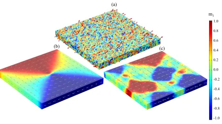
and d) the grain structure. ... 38 Figure 4.2 Schematic illustration of the boundary conditions and the simulation domains. ... 41 Figure 4.3 (a) Random initial condition for the magnetization unit vector and equilibrium

spontaneous domain structure for unstrained randomly-textured (b) NFO, and (c) CFO films. The arrows point to the directions of the magnetization vectors and different colors denote the values of m1 component of the magnetization. The film dimensions are 850 × 850 × 75 nm3 and 550 × 550 × 50 μm3 for

NFO and CFO, respectively. ... 44 Figure 4.4 Schematic representation of the polycrystalline film and stereographic

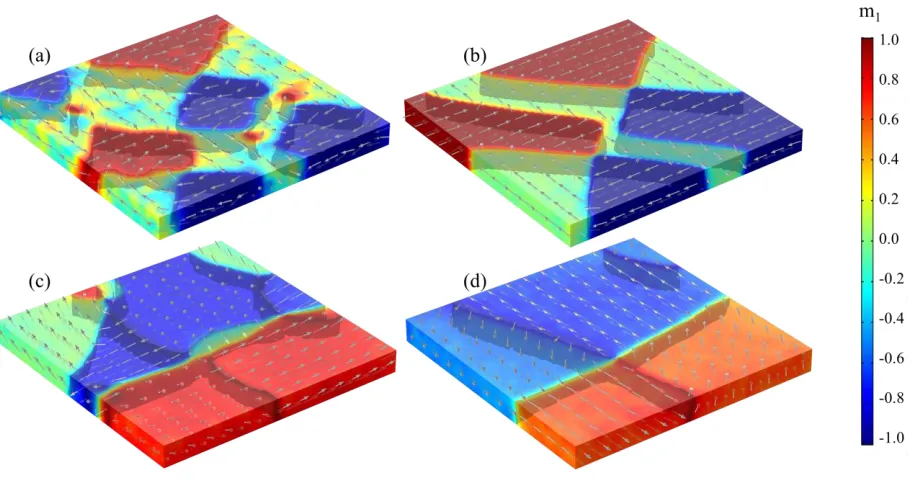
x Figure 4.5 Spontaneous domain structure of unstrained CFO films with (a)

randomly-oriented, (b) (100)-textured, (c) (111)-textured, and (d) (110)-textured microstructure. The arrows represent the magnetization vectors and different colors denote the values of m1 component of the magnetization. The interfaces between magnetic domains are marked by dark surfaces. The film dimensions

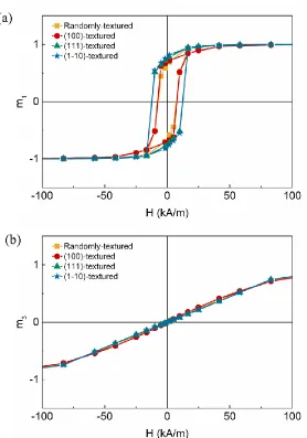
are 550 × 550 × 50 nm3. ... 47 Figure 4.6 (a) In-plane and (b) out-of-plane magnetization hysteresis curves of unstrained

randomly-oriented, (100)-textured, (111)-textured, and (110)-textured NFO

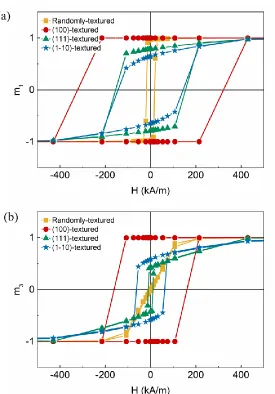
films. ... 49 Figure 4.7 (a) In-plane and (b) out-of-plane magnetization hysteresis curves of unstrained

randomly-oriented, (100)-textured, (111)-textured, and (110)-textured CFO

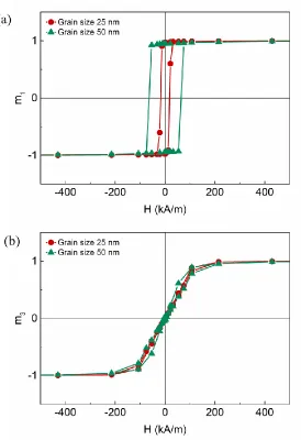
films. ... 50 Figure 4.8 (a) In-plane and (b) out-of-plane magnetization hysteresis curves of unstrained

randomly-oriented CFO films with grain sizes of 25 and 50 nm. ... 51 Figure 4.9 Spontaneous domain structure of NFO for a biaxial substrate-induced strain

values of (a) -0.50%, (b) -0.25%, (c) 0.00%, (d) 0.25%, and (e) 0.50%. The arrows represent the magnetization vectors and different colors denote the values of m3 component of the magnetization. The film dimensions are 850 ×

850 × 75 nm3. ... 53 Figure 4.10 (a) In-plane and (b) out-of-plane magnetization hysteresis curves of NFO

films with biaxial substrate-induced strain values of -0.50%, -0.25%, 0.00%,

0.25%, and 0.50%. ... 54 Figure 4.11 Comparison of the modeling results with experimental data for (a) in-plane

magnetizing of randomly-oriented NFO film [66], (b) in-plane magnetizing of textured NFO film [67], and (c) out-of-plane magnetization of

(111)-textured NFO film [67]. ... 56 Figure 5.1 Finite element domain and mesh for a) Eq. (3.20), b) Eq. (3.18), and c) Eq.

(3.19). ... 62 Figure 5.2 Patterned nanostructures with different geometric parameters. ... 65 Figure 5.3 Comparison of in-plane magnetization curves of striped and unpatterned thin

films for different material parameters and 0.00% biaxial strain. ... 66 Figure 5.4 Comparison of out-of-plane magnetization curves of striped and unpatterned

thin films for different material parameters and 0.00% biaxial strain. ... 67 Figure 5.5 Comparison of in-plane and out-of-plane magnetization curves of striped and

unpatterned thin films for different material parameters and 0.10% biaxial

strain. ... 68 Figure 5.6 Comparison of in-plane magnetization curves of stripe patterning with

different geometric parameters: (a) 𝜆100(2)𝐾1(1)𝑀𝑠(1), (b) 𝜆100(2)𝐾1(1)𝑀𝑠(2), (c) 𝜆100(2)𝐾1(1)𝑀𝑠(1), (d) 𝜆100(2)𝐾1(1)𝑀𝑠(2), (e) 𝜆100(2)𝐾1(2)𝑀𝑠(1), and (f)

xi Figure 5.7 Comparison of in-plane magnetization curves of square patterning with

different geometric parameters: (a) 𝜆100(2)𝐾1(1)𝑀𝑠(1), (b) 𝜆100(2)𝐾1(1)𝑀𝑠(2), (c) 𝜆100(2)𝐾1(1)𝑀𝑠(1), (d) 𝜆100(2)𝐾1(1)𝑀𝑠(2), (e) 𝜆100(2)𝐾1(2)𝑀𝑠(1), and (f)

𝜆100(2)𝐾1(2)𝑀𝑠(2). ... 72 Figure 5.8 Distribution of the stray field after removing the applied field for

𝜆100(2)𝐾1(1)𝑀𝑠(2). ... 74 Figure 5.9 Spontaneous domain structures at zero external magnetic field for

𝜆100(2)𝐾1(1)𝑀𝑠(2). ... 75 Figure 5.10 Snap-shots of the domain structure at remanence and coercivity for

𝜆100(2)𝐾1(1)𝑀𝑠(2). ... 78 Figure 6.1 a) Vertical (nano-pillars) and b) horizontal (laminated) connectivity schemes

in biferroic heterostructures along with c) proposed design with patterned

interface. ... 82 Figure 6.2 Finite element domain and mesh for a) Eq. (3.20), b) Eq. (3.18), and c) Eq.

(3.19). ... 87 Figure 6.3 Considered geometries for biferroic heterostructures; laminated films with a)

flat interface, b) stripe patterns, c) square patterns. ... 90 Figure 6.4 Comparison of in-plane and out-of-plane magnetization curves in unpolarized

biferroic heterostructures with different interfacial patterning; a1) Sub-NFO-PTO (in-plane magnetization), a2) Sub-PTO-NFO (in-plane magnetization), b1) Sub-NFO-PTO (out-of-plane magnetization), b2) Sub-PTO-NFO

(out-of-plane magnetization). ... 92 Figure 6.5 Comparison of in-plane magnetization curves in biferroic heterostructures

with ferroelectric layer polarized in different directions; a1) Sub-NFO-PTO with flat interface, a2) Sub-PTO-NFO with flat interface, b1) Sub-NFO-PTO with stripe-patterned interface, b2) Sub-PTO-NFO with stripe-patterned interface, c1) Sub-NFO-PTO with square-patterned interface, and c2)

Sub-PTO-NFO with square-patterned interface. ... 93 Figure 6.6 Comparison of out-of-plane magnetization curves in biferroic heterostructures

with ferroelectric layer polarized in different directions; a1) Sub-NFO-PTO with flat interface, a2) Sub-PTO-NFO with flat interface, b1) Sub-NFO-PTO with stripe-patterned interface, b2) Sub-PTO-NFO with stripe-patterned interface, c1) Sub-NFO-PTO with square-patterned interface, and c2)

Sub-PTO-NFO with square-patterned interface. ... 95 Figure 6.7 Interfacial strain along the polarization directions for Sub-NFO-PTO

composite films. ... 97 Figure 6.8 Interfacial strain along the polarization directions for Sub -PTO-NFO

1 Chapter 1Introduction

1.1 Motivations

Multiferroic materials exhibit multiple ferroic orders simultaneously. Biferroic magnetoelectric systems are the widely used class of these materials that poses ferromagnetic and ferroelectric order coupling. The magnetoelectric coupling enables controlling dielectric-polarization via applying magnetic field or manipulating material magnetization through application of electric field. The coexistence of ferroelectric and ferromagnetic orders was studied in both single-phase materials with direct coupling between the two ferroic orders [1,2] and composite materials with strain-mediated coupling [3,4]. The room temperature response obtained in strain-mediated coupling is orders-of-magnitude higher than that in single-phase materials, and thus potential for applications is higher. Progress has been sporadic, however, due to the complexity of the composite materials design, especially at small scales.

2 consistent with the ideal geometry for magnetoelectric coupling. In addition, the leakage problem is eliminated due to its layered structure.

1.2 Overview

3 Chapter 2Magnetoelectric biferroic materials

2.1 Introduction

The focus in the field of material science over the past decades was on the invention of new class of materials known as functional materials. A material is generally considered to be functional if it poses certain physical properties that can be utilized for particular applications. One new class of functional materials is multiferroic magnetoelectric heterostructures. These materials are developed in response to the growing demand for miniaturization and power saving in electronic devices. The aim of this chapter is to provide a brief review of the concept of multiferroicity and magnetoelectric coupling with a focus on magnetoelectric biferroic composites.

2.2 Definitions and concepts

Ferroic materials are defined as materials that when undergo below a transition temperature show spontaneous long-range ordering of a macroscopic physical property [1]. As showing in Figure 2.1, this ordering leads to formation of domain structure which can be switched historically by the application of an external field. Ferroic materials are categorized as ferromagnetic, ferroelectric, ferroelastic and ferrotoroidic materials. There are also antiferroic materials in which the ordering is cancelled out; examples are antiferromagnetic and antiferroelectric materials.

Figure 2.1 a) Schematic illustration of ferroic ordering for ferroelectric and ferromagnetic materials, b) historical switching of domain structure (after [1])

4 The following definitions are given to describe each class of ferroic materials [8].

 Ferroelectricty is observed in materials that exhibit stable spontaneous polarization

which can be switched by the application of electric field.

 Antiferroelectricity is observed in materials that form order dipole moments but

cancel each other completely within each crystallographic unit cell. The macroscopic net polarization is zero.

 Ferromagnetism is attributed to a material that experience stable spontaneous

magnetization that can be switched by the application of a magnetic field.

 Antiferromagnetism is seen in materials that have ordered magnetic moments but

they cancel each other completely within each magnetic unit cell. The macroscopic net magnetization is zero.

 Ferrimagnetism is incomplete antiferromagnetic cancellation in a way that there is

a net magnetization that, similar to ferromagnetic materials, can be switched by the application of a magnetic field.

 Ferroelasticity results in spontaneous deformation that is stable and can be switched

by the application of stress field.

 Ferrotoroidicity is observed in materials that possess a stable and spontaneous order

parameter that is taken to be the curl of a magnetization or polarization. By analogy with other ferroic materials, this order parameter needs to be switchable.

5 Magnetoelectric coupling is an independent concept that describes controlling dielectric-polarization via applying magnetic field or manipulating material magnetization through application of electric field. This phenomenon is not exclusive to multiferroics and may exist among other class of materials such as paramagnetic ferroelectrics. Figure 2.2 shows the relationship between multiferroic and magnetoelectric materials and the area that these two overlap.

Figure 2.2 The relationship between multiferroic and magnetoelectric materials [8].

The magnetoelectric (ME) biferroic materials are referred to materials that exhibit coupling between the co-existing ferroelectric and ferromagnetic ordering. This notion was originally studied in single-phase materials with direct coupling between the two ferroic orders [1,8]. The room temperature response obtained in such materials, however, is not high enough for most technological applications due to having either low permittivity or low permeability [3]. The alternative approach is to utilize the magnetoelastic and electromechanical coupling in magnetostrictive1 and piezoelectric2 materials to make synthetic biferroic heterostructures. The

1 _{Magnetostriction describes a change in strain as a quadratic function of applied magnetic field, or change}

in magnetization as a quadratic function of applied stress [8].

2 _{Piezoelectricity describes a change in strain as a linear function of applied electric field, or change in}

6 strain transfer across the interface of the two phases will allow the coupling of ferromagnetic and ferroelectric orders (Figure 2.3).

Figure 2.3 Schematic illustration of strain mediated ME coupling [3].

ME biferroic heterostructures have been made in the form of bulk composites as well as composite films [3,5,12,13]. The response obtained through strain-mediated coupling is orders-of-magnitude higher than in single-phase materials, and thus the potential for applications is enhanced greatly.

2.3 Historical background

The history of ME biferroicity starts in 1894 when Pierre Curie stated that “The applications of symmetry conditions provide us that a body with an asymmetric molecule gets electrically polarized when placed in a magnetic field…. And perhaps magnetically when placed in an electric field” [14]. The concept of symmetry was used to predict the existence of the ME

7 of papers reporting the observation of ME effect in many single crystal and polycrystalline materials [14].

The chart in Figure 2.4 summarizes the evolution of multiferroic magnetoelectricity ever since the prediction of the concept by Pierre Curie. The main applications, advantages and/or disadvantages, research emphasis or challenges of each generation are also included in this figure [17].

Figure 2.4 Evolution on the development of ME materials: from single-phase compounds to multi-phase ferromagnetic/ferroelectric composites and from bulk laminates to micro-/nano-thin films [17].

As mentioned previously, ME biferroicity in single phase materials is mostly observed at low temperatures. Bismuth ferrite (BiFeO3) is one of the few materials that shows room temperature ME biferroicity [8]. The coupled orders, however, are ferroelectricity and antiferromagnetism. In other words, it exhibits magnetically switchable electric polarization, but the net magnetization is zero. This antiferromagnetic behavior is a big shortcoming from technological point of view.

8 of BaTiO3-CoFe2O4. The obtained ME coefficient was hundreds of times larger than that of single-phase multiferroics [10]. However, since the unidirectional solidification method is very costly, this new field of ME composite went dormant for the next 20 years. In early 1990s, the conventional sintering process was used to prepare more cost-effective ME composites. Since then numerous efforts have gone into developing new fabrication methods in order to improving the ME coupling and increase the ME coefficient. Along with the progress in processing methods, analytical models were developed to predict and study the mechanisms that result in ME effect [18]. This expedited the advancement in experimental techniques.

2.4 The origin of ferromagnetism

2.4.1 Diamagnetic and paramagnetic materials

Magnetization is the manifestation of the electric charges in motion [19]. On this basis, electrons orbiting the nucleus in atom and electrons spinning themselves will produce magnetic moment. The magnetic moment due to electron spin is parallel to the axis of the spin and the magnetic moment due to electron orbital motion is normal to the plane of the orbit. The vector field that explains the density of the magnetic moments is called magnetization.

The magnetic moment of an atom is vector sum of spin and orbital magnetic moments of all electrons in atom. There are two possible scenarios:

1. There is no unpaired electrons in the outer orbital shell and as a result the magnetic moments of electrons are canceled and the net magnetic moment of the atom is zero.

9 The former leads to definition of diamagnetic materials. Electrons which fill closed shell in an atom orient their spin and orbital magnetic moment in a way that the atomic magnetic moment is zero. Monoatomic rare gases such as helium (He), or polyatomic gases such nitrogen (N2) are good examples.

Although, the net magnetization of diamagnetic materials is zero, application of the applied field induces negative magnetic moments in the opposite direction. A repulsive force builds up in the atom resisting the magnetic field to lower the amount of current orbiting around the nucleus by reducing the electron speed. This translates into the negative magnetization. This effect which is called diamagnetic effect is not exclusive to diamagnetic materials. But since it is very week, it can only be detected in diamagnetic materials. For this reason, the magnetic susceptibility, which is the measure of the amount of magnetic moments induced in a material by application of the magnetic field, is negative in diamagnetic materials. .

10 2.4.2 Ferromagnetic materials

In some paramagnetic materials, such as iron, nickel and cobalt, the interatomic distance is so small that below a certain temperature known as Curie temperature, the magnetic moments of the electrons in each atom is coupled to the magnetic moments of the electrons in neighboring atoms. When the atoms get closer to each other they start to exchange the electrons that orbit their outer shell. Such exchange interaction is stronger between atoms of iron, nickel and cobalt and develops a force between the unpaired electrons in 3d shell aligning their spin in the same direction. As a result, the net magnetic moment of atom is much larger than the regular paramagnetic materials.

This strong net magnetic moment and interaction between them result in parallel alignment of magnetic moments in the material even in the absence of magnetic field (see Figure 2.5a). This is called spontaneous magnetization and the materials that show this behavior are classified as ferromagnetic materials.

The regions of the material in which the magnetic moments are aligned parallel to each other are called domains. In order to reduce the free energy of the system, there should be more than one domain in materials that are larger than a critical size. The magnetization vector in each domain is usually normal or antiparallel to the magnetization vector in the neighboring domains. These domain are separated by domain walls.

11 The important characteristic of ferromagnetic materials is the hysteretic losses during the magnetization process. When a ferromagnetic materials is cooled down from Curie temperature, domain structures will form with a magnetization in each domain equal to the maximum possible amount of the magnetization that can be reached. This is known as saturation magnetization. Usually, the domain structure forms in a way that the net magnetization of the material is zero. As it is shown in see Figure 2.5b, by applying an external field, the net magnetization increases non-linearly until it reaches to its saturation level. Removing the field, the material does not go back to its original un-magnetized state, rather it holds a non-zero net magnetization which is called remanent magnetization. In order to reduce the net magnetization to zero, a negative external field should be applied which is known as coercive field.

2.4.3 Antiferromagnetic and ferrimagnetic materials

It should be emphasized that the interatomic distance is the only contributor for ferromagnetic behavior and it goes away when the temperature reaches the Curie temperature. Above this temperature a ferromagnetic material becomes paramagnet. In some materials such as Mn, the interatomic spacing is so small that the exchange interaction between atoms results in alignment of electron spins in opposite directions (see Figure 2.5a). This phenomenon, which is called antiferromagnetism, results in complete cancelation of magnetic moments and hence produces zero net magnetization.

12

Figure 2.5 a) Bethe–Slater curve showing the relationship between interatomic distance and exchange interaction that leads to ferromagnetic behavior in Ni, Co, and Fe, and antiferromagnetic behavior in Mn.

b) Typical hysteresis curve for ferromagnetic materials showing the saturation magnetization Ms, the

remanent magnetization Mr, and coercive field Hc. The plots are taken from [19].

2.4.4 Magnetostriction

Depending on the crystal structure, in most materials the magnetic moment due to electron’s spin is much stronger than that due to electron’s orbital motion. Accordingly, in most

calculations the orbital magnetic moment is ignored. For some materials, such as ferromagnets, the strength of the orbital magnetic moment is not negligible and hence its presence is very important because the interaction between the magnetic moment due to electron’s spin with that due to electron’s orbital motion results in spin-orbit coupling. Since the orbital motion of the

electron is dictated by the lattice structure, the spin-orbit coupling links the electronic magnetic moment to crystal structure. In other words, changing the orientation of the magnetic moments will result in deformation in lattice structure. This links the mechanical strain and magnetization in ferromagnetic materials and is called magnetostriction.

13 2.5 The origin of ferroelectricity

2.5.1 Dielectric and paraelectric materials

A dielectric material is an electrical insulator in which electrical dipole moments can be induced by the application of electric field. The vector field that expresses the density of induced electrical dipole moments is called polarization. One of the important properties of dielectric materials is dielectric constant K, also known as relative permittivity, which is the measure of the materials ability to store charge. In most dielectric materials the polarization achieved is linearly proportional to the applied field and the dielectric constant is the constant of the proportionality.

There are four main mechanisms for polarization in dielectric materials [20]. 1. Electronic polarization

2. Ionic polarization

3. Orientational polarization 4. Spontaneous polarization

Electronic polarization occurs in all materials and arises from field induced changes in symmetrical distribution of electron cloud around each atom. Ionic polarization takes place in materials made of two or more different kinds of atoms that share their valence electrons and form an ion. Similar to electronic polarization, the ionic polarization is induced by the application of electric field. Both of these polarization mechanism seek lower potential energy by elastically displacing the valence electron clouds from their original thermal equilibrium state to a new equilibrium state. The new equilibrium state is only slightly dependent on thermal agitations.

14 are randomly distributed in the material and hence the net polarization is equal to zero. An electric field will cause them to change their orientations which results in the rotation of the molecule. This process that is called orientational polarization is strongly temperature dependent. After the electric field is removed the ordered orientations go back to their disordered state resulting in zero net polarization. This temporary polarization of the material in the presence of electric field is called paraelectricity and is analogous to the concept of paramagnetism.

As paramagnetism corresponds to positive magnetic susceptibility, paraelectricity corresponds to positive electric susceptibility. It should be noted that the there is no counterpart to diamagnetization in dielectric materials and unlike diamagnetic materials that have negative magnetic susceptibility, the electric susceptibility in dielectric materials is not negative.

2.5.2 Pyroelectric and piezoelectric materials

The formation and rotation of electrical dipole moments is coupled with the lattice structure in crystals. The lattice structure is also linked to thermal agitations and mechanical strain. As a result, the formation and rotation of the electrical dipole moments is coupled to temperature field and strain field. The coupling of the dipole moments with temperature is expressed with pyroelectric effect and its coupling with strain is expressed by piezoelectric effect.

2.5.3 Ferroelectric materials

15 electrical dipole moments. The dipole moment in each unit cell is coupled with the dipole moments of the neighboring unit cells so that they tend to be aligned parallel. This process is called spontaneous polarization.

The chain of unit cells with coupled dipole moments will form a domain of ordered dipole moments. This is similar to formation of magnetic domains in ferromagnetic materials. However, the spontaneous polarization is the characteristic of pyroelectric materials and is not exclusive to ferroelectric materials. Ferroelectricity, requires the spontaneous polarization to be reversible by the application of external electric field. The difference between pyroelectricity and ferroelectricity is shown in Figure 2.6.

Figure 2.6 Schematic representation of the fundamental polarization mechanisms and crystal symmetry in dielectric materials [21].

16 is no iron atom in ferroelectric materials. In fact, ferroelectricity is discovered much later than ferromagnetism. Thus, the prefix ferro- in ferroelectricity implies similarity in characteristics to ferromagnetism.

Just like the ferromagnetic materials, ferroelectric materials show hysteretic behavior with saturation polarization, remanent polarization and coercive field. In similar sense, there are materials that show antiferroelectric behavior (see Figure 2.6).

2.5.4 Crystal symmetry

It can be imagine that materials exhibiting ferroelectric behavior must have crystalline order. In fact all ferroelectric materials are either single crystals or polycrystalline solids composed of crystallites. On a similar basis, all the mechanisms for polarization of dielectric materials mentioned above can be explained by the symmetry in crystalline structure.

According to the symmetry elements of translational position and orientation, there are 230 space groups. Ignoring translational reputation, these 230 space groups are reduced to 32 point groups that are based on orientation only. These 32 point groups are subdivisions of seven basic crystal systems. In the order of the lowest symmetry to the highest symmetry, these seven basic crystalline structures are triclinic, monoclinic, orthorhombic, tetragonal, trigonal (rhombohedral), hexagonal, and cubic [22].

17 possess unique polar axis that can be spontaneously polarized. These 10 classes show piezoelectric and pyroelectric behavior at the same time. There is only one subgroup within this 10 point groups that is capable of reversing the spontaneous polarization along the polar axis. This is the only symmetry that fulfils the requirement for ferroelectricty.

2.6 ME biferroic heterostructures 2.6.1 Strain mediated ME coupling

ME biferroic composites that are made by combining ferromagnetic and ferroelectric materials possess very strong ME coupling which is several orders of magnitude higher than that in single compounds and is sustainable at room temperature [5].

18

Figure 2.7 Schematic illustration of strain-mediated ME effect in a composite system consisting of a magnetic layer (purple) and ferroelectric layer (pink) [5].

2.6.2 Connectivity schemes

Advances in thin-film growth techniques have enabled development of nano-structured multiferroic composites. Experiments show that such materials could exhibit more promising ME effect compared to their bulk counterparts [3,5,7,10,23]. Unlike the bulk counterparts where the connectivity between the two phases are not very strong1, the two phases in nano-structured films are directly connected in atomic level [5,8]. This implies stronger coupling between the phases. In addition, larger electric field can be comfortably applied to thin-films as they require smaller bias voltages [3]. Moreover, the small scale nature of these materials allows more precise control over parameters during fabrication process which enable tuning of the properties toward targeted behavior [5].

1 _{Connectivity between the phases in bulk composites is usually achieved via polymeric resins or sintering}

19 The ME composites are generally classified based on connectivity of the phases that constitute the material. The classification follows the notation of Newnham [24] in which the design is referred to as x-y where x is the dimension of the connectivity in the first phase and y is the dimension of the connectivity in the second phase. The most widely employed designs are shown in Figure 2.8.

Figure 2.8 Schematic illustration of three kinds of ME composite nanostructures with common connectivity schemes. (a) 0-0 non-continuous inclusions embedded in a continuous matrix (3), (b) 2-2 horizontal laminated layers of ferroelectric and ferromagnetic materials, and (c) 1-3 vertical pillars of one

phase embedded in a matrix of another phase [5].

20 overall ME coupling [7,10] If the leakage problem is eliminated, larger interfacial surface area in these systems leads to even more enhanced ME coupling that can exceed the values reported for balk composites [2,3].

Since the ferromagnetic phases are not connected to the electrodes in the laminated structure, the leakage problem does not exist in 2-2 systems. Moreover, the fabrication process for 2-2 systems are much easier which makes these design configuration even more desired.

2.6.3 ME coefficient

The figure of merit that quantifies the coupling strength between the electric and magnetic field in synthetic biferroic ME materials is ME coefficient which is a product tensor property [7,10]. Direct ME coefficient (αdirect) measures the efficacy of controlling the electric polarization through the applied magnetic field.

𝛼_{𝑑𝑖𝑟𝑒𝑐𝑡}= 𝜕𝑃

𝜕𝐻 (2.1)

The direct ME voltage coefficient (αE), which is the ratio of output electric field produced to the applied magnetic field, is another metric.

𝛼_𝐸 = 𝜕𝐸

𝜕𝐻 (2.2)

Electric field control of magnetization is quantified by the converse ME coefficient (αconverse) that measures the appearance of the magnetization upon applying electric field.

𝛼_{𝑐𝑜𝑛𝑣𝑒𝑟𝑠𝑒} = 𝜕𝑀

𝜕𝐸 (2.3)

21 1) Parameters related to constituents of the composite and their independent

performance.

2) Parameters related to connectivity and interfacial bonding, including the interfacial geometry and the presence of intermediate layers.

2.6.4 Material selection

The parameters that should be considered for selecting constituents of biferroic ME heterostructures include electric permittivity, magnetic permeability, ordering temperatures, remanent polarization, remanent magnetization, coercive electric field, coercive magnetic field, dielectric losses, electrical resistivity, and piezoelectric and magnetostrictive constants [3]. In addition, the conditions required to synthesize the phases with the desired textures and to process the integrated composite must be factored.

It should be noted that the ultimate purpose of design plays a significant role in determining what parameters should be considered, whether it is designed for magnetic control of polarization or electric control of magnetization. Figure 2.9 summarizes the best values of ME coefficient obtained for different combinations of materials in bulk and film-based ME composites having 0-3, 1-0-3, and 2-2 connectivity [4].

22

Table 2.1 List of well-known piezoelectric and magnetostrictive materials used as constituents of ME composites. The list is taken from [3].

Piezoelectric Phase Magnetostrictive Phase

Lead-based: Metals:

Pb(Zr,Ti)O3 (PZT) Fe, Co, Ni

Pb(Mg1/3Nb2/3)O3-PbTiO3 (PMN-PT) Alloys:

Pb(Zn1/3Nb2/3)O3-PbTiO3 (PZN-PT) FeNi-based

Pb(Mg1/3Nb2/3)y (ZrxTi1−x)1−yO3 (PMN–PZT) FeCo-based

Pb(In1/2Nb1/2)O3-Pb(Mg1/3Nb2/3)O3-PbTiO3 (PIN-PMN-PT) CoNi-based

Ni2MnGa

Permendur (FeCoV)

Lead-free: Galfenol (FeGa), FeGaB

BaTiO3 (BTO)-based Samfenol (SmFe2)

(K0.5Na0.5)NbO3 (KNN)-based Terfenol-D (Tb1-xDyxFe2)

Na0.5Bi0.5TiO3 (NBT)-based Fe-based metallic glasses (FeBSi, FeBSiC, FeCoB,

FeCoSi, FeCoSiB, FeCuNbSiB)

Others:

AlN Ceramics:

ZnO Fe3O4

(Sr, Ba)Nb2O5 Zn0.1Fe2.9O4 (ZFO)

Ba1-xSrxTiO3 (BSTO) LaxSryMnO3 (LSMO)

Bi1-xSrxTiO3 (BST) LaxCayMnO3 (LCMO)

La3Ga5.5SiO14 (LGS) Ferrites or doped Ferrites (e.g., NiFe2O4 (NFO),

CoFe2O4 (CFO), Li ferrite, Cu ferrite, Mn ferrite)

La3Ga5.5Ta0.5O14 (LGT)

Polyurethane (PU)

Polyvinylidene difluoride (PVDF)

Various piezoelectric and magnetostrictive phases have been used for construction of ME composites. Some of these materials are listed in Table 2.1. Among the piezoelectric materials, PZT-based ceramics have been widely employed to fabricate the ME composites due to their low cost, high piezoelectric response, and flexibility in modifying the composition. For the magnetostrictive phase, terfenol-D with high magnetostriction and metglass (amorphous Fe-alloy) with high magnetic permeability have been the most used materials [3].

2.6.5 Other mechanisms contributing to ME effect

23 this, the effect of spontaneous polarization/magnetization should also be taken into account as the obtained domain structure is relatively comparable to the size scale of the films [5,23].

In addition to the strain mediated coupling, studies have reported two other mechanisms that contribute to the converse ME effect; charge-mediated and exchange-bias mediated ME effects [7].

In the laminated heterostructures containing ultrathin ferromagnetic films, an electric field could result in the accumulation of spin-polarized electrons or holes at the interface. The change in the number of free carriers produces a change in the surface magnetization and the surface magnetocrystalline anisotropy [7].

The exchange bias, resulting from the exchange coupling between the uncompensated interfacial spins of the antiferromagnetic and the spins of the ferromagnetic layer, has also been employed for electric field control of the magnetic properties in the ferromagnetic films [7].

2.7 Applications

The potential applications of different ME composite depend on the type of the ME coupling. The most popular proposed applications are magnetic sensors, electric sensors, biomedical applications, magnetoelectric recording, energy harvesters, magnetic antenna, high-frequency inductors, and high-high-frequency signal processing devices [1,3,7,10,25]. The main advantages of using multiferroic magnetoelectricity for these applications are design miniaturization, lowering power consumption and improving performance speed [7].

2.8 Modeling of ME behavior in biferroic films 2.8.1 Green’s function method

Early attempts to model biferroic ME films were based on the Green’s function approach

24 capable of simulating the complexity of ferroelectric and ferromagnetic domain structures. Since the relative sizes of the films are very close the domain sizes, any assumption that neglects domain structure effects is intrinsically inaccurate. An alternative approach is the phase-field method which has been proven to be a powerful tool for studying the ferroelectric and ferromagnetic ordering [28–30].

2.8.2 Phase-field methods

25 Chapter 3 Phase-field micromagnetics: a continuum thermodynamics formulation 3.1 Free energy functional

The free energy functional for phase-field micromagnetic modeling is a state function for magnetization derived from continuum thermodynamics and crystal symmetry considerations. Assuming the temperature is constant and well below the Curie temperature it can be written as:

ℎ = ℎ(𝜀_𝑖𝑗, 𝐻_𝑖, 𝑚_𝑖, 𝑚_𝑖,𝑗) (3.1)

where the primary field variables are the strain field tensor εij, magnetic field vector Hi, magnetization unit vector (also known as direction cosines) mi, and its gradient mi,j. Standard index notation with summation convention over repeated indices is used throughout this document. The indices are running over the range of 1-3. The comma in the subscript denotes partial differentiation with respect to spatial coordinate xi.

Under the assumption of linear kinematics, the strain tensor in a material body can be calculated from mechanical displacement ui.

𝜀_𝑖𝑗 =1

2(𝑢𝑖,𝑗+ 𝑢𝑗,𝑖) (3.2)

The magnetic field and magnetization unit vector are related to the magnetic field Bi, via

𝐵𝑖 = 𝜇0(𝐻𝑖+ 𝑀𝑠𝑚𝑖) (3.3)

μ0 is the permeability of the free space and Ms is the saturation magnetization. The magnetic

field can be expressed as the gradient of the magnetic scalar potential ϕ.

𝐻𝑖 = −𝜙,𝑖 (3.4)

Assuming constant saturation magnetization

𝑚_𝑖 = 𝑀𝑖

26 where Mi are the components of the magnetization field vector. The modulus of the magnetization vector is assumed to be constant and equal to the saturation magnetization. Therefore, it is more convenient to use the magnetization unit vector as the primary order parameter.

The total free energy density functional for phase-field micromagnetics modeling consists of contributions from magnetocrystalline anisotropy energy haniso, exchange energy hexch, elastic energy helastic, and magnetostatic energy hmagnetostatic. The competition between these four energy terms defines the magnetic state of the material:

ℎ = ℎ𝑎𝑛𝑖𝑠𝑜+ ℎ𝑒𝑥𝑐ℎ+ ℎ𝑒𝑙𝑎𝑠𝑡𝑖𝑐+ ℎ𝑚𝑎𝑔𝑛𝑒𝑡𝑜𝑠𝑡𝑎𝑡𝑖𝑐 (3.6) The magnetocrystalline anisotropy energy arises because the magnetization process depends on the crystallographic directions. Ignoring the higher order terms, the magnetocrystalline anisotropy energy for cubic symmetry is

ℎ𝑎𝑛𝑖𝑠𝑜 = 𝐾1(𝑚12𝑚22+ 𝑚12𝑚32+ 𝑚22𝑚32) + 𝐾2(𝑚12𝑚22𝑚32) (3.7) Here K1 and K2 are denoted as the first and second anisotropy constants. Depending on their sign and magnitude, Eq. (3.7) creates energy wells that favor certain magnetization directions. The exchange energy or gradient energy is related to the inhomogeneous distribution of the magnetization and originates from a short-range interaction between magnetic moments while tending to keep them parallel. The mathematical expression is defined as the square of the spatial gradient of the magnetization directions:

ℎ_{𝑒𝑥𝑐ℎ} = 𝐴_{𝑒𝑥𝑐ℎ}(𝑚_1,12 + 𝑚_1,22 + 𝑚_1,32 + 𝑚_2,12 + 𝑚_2,22 + 𝑚_2,32 + 𝑚_3,12 + 𝑚_3,22 + 𝑚_3,32 ) (3.8) where Aexch is the exchange stiffness constant.

27 accompanied by elastic strains. The resultant elastic energy contains a positive term for pure elastic strains and a negative term for quasi-plastic magnetostrictive strains [47].

ℎ_{𝑒𝑙𝑎𝑠𝑡𝑖𝑐} = 1

2𝐶𝑖𝑗𝑘𝑙(𝜀𝑖𝑗 − 𝜀𝑖𝑗 𝑚_)(𝜀

𝑘𝑙− 𝜀𝑘𝑙𝑚) = 1

2𝐶𝑖𝑗𝑘𝑙𝑒𝑖𝑗𝑒𝑘𝑙 (3.9)

where Cijkl is the fourth order elastic stiffness tensor, εij is the pure elastic strain, εm

ij is the magnetostrictive strain, and eij = εij - εmij. The magnetostrictive strain is a function of magnetostriction constants and components of the magnetization unit vector. In the case of a cubic crystal it is given by:

𝜀_𝑖𝑗𝑚 =

[ 3

2𝜆100(𝑚1 2₋1

3) 3

2𝜆111𝑚1𝑚2

3

2𝜆111𝑚1𝑚3 3

2𝜆111𝑚2𝑚1 3

2𝜆100(𝑚2 2₋1

3) 3

2𝜆111𝑚2𝑚3 3

2𝜆111𝑚3𝑚1

3

2𝜆111𝑚3𝑚2 3

2𝜆100(𝑚3 2₋1

3)]

(3.10)

where λ100 and λ111 are magnetostriction constants corresponding to the displacement due to saturation along <100> and <111> directions, respectively. Given the symmetry in crystal classes, most elements of the stiffness tensor are zero. For a cubic crystal, only three independent elastic constants are needed. Using the Voigt notation, Eq. (3.9) can be re-written as

ℎ_{𝑒𝑙𝑎𝑠𝑡𝑖𝑐} = 1

2𝑐11(𝑒11 2 _{+ 𝑒}

222 + 𝑒332 ) + 𝑐12(𝑒11𝑒22+ 𝑒22𝑒33+ 𝑒11𝑒33) + 𝑐44(𝑒122 + 𝑒212 + 𝑒232 + 𝑒322 + 𝑒132 + 𝑒312 )

(3.11)

28 ℎ_{𝑒𝑙𝑎𝑠𝑡𝑖𝑐} = 1

2𝑐11(𝜀11 2 _{+ 𝜀}

222 + 𝜀332 ) + 𝑐12(𝜀11𝜀22+ 𝜀22𝜀33+ 𝜀11𝜀33) + 𝑐₄₄(𝜀₁₂2 _{+ 𝜀}

212 + 𝜀232 + 𝜀322 + 𝜀132 + 𝜀312 ) −3

2𝜆100(𝑐11− 𝑐12)(𝜀11𝑚1 2_{+ 𝜀}

22𝑚22+ 𝜀33𝑚32)

− 3𝜆₁₁₁𝑐₄₄(𝜀₁₂𝑚₁𝑚₂+ 𝜀₂₁𝑚₂𝑚₁+ 𝜀₂₃𝑚₂𝑚₃+ 𝜀₃₂𝑚₃𝑚₂+ 𝜀₁₃𝑚₁𝑚₃ + 𝜀₃₁𝑚₃𝑚₁)

(3.12)

The energy landscape associated with the self-demagnetization field and external field is called the magnetostatic interaction energy. The demagnetization field energy is the result of the interaction of the magnetization with the magnetic field generated by the magnetic body itself. The competition between the long-range magnetostatic energy and short-range exchange energy forms the magnetic domain structure. It should be noted that the magnetostatic energy includes both the energy stored in the material as well as in the free space.

ℎ𝑚𝑎𝑔𝑛𝑒𝑡𝑜𝑠𝑡𝑎𝑡𝑖𝑐 = −𝜇0𝑀𝑆(𝐻1𝑚1+ 𝐻2𝑚2+ 𝐻3𝑚3) − 1 2𝜇0(𝐻1

2_{+ 𝐻}

22+ 𝐻32) (3.13) Summing the above energy terms, the total magnetic free energy density functional for a cubic crystal is obtained.

3.2 Field equations

The field equation for the stress field equilibrium is based on the conservation of linear and angular momentum. Assuming small deformations and neglecting the body forces, the quasi-static mechanical equilibrium in a material body takes the following form for Cauchy stress tensor σij

𝜎𝑖𝑗,𝑗 = 0 (3.14)

The magnetic field in the material body (and also in the free space) is governed by Gauss' Law for magnetism which ensures the solenoidality of the magnetic induction:

29 The stress and magnetic field induction can be calculated using derivatives of the free energy density functional with respect to the strain and magnetic field, respectively,

𝜎_𝑖𝑗 = 𝜕ℎ

𝜕𝜀_𝑖𝑗 (3.16)

𝐵𝑖 = − 𝜕ℎ

𝜕𝐻_𝑖 (3.17)

Substituting Eq. (3.16) into (3.14) and Eq. (3.17) into Eq. (3.15), the final form of the field equations are written as

𝜕 𝜕𝑥_𝑗(

𝜕ℎ

𝜕𝜀_𝑖𝑗) = 0 (3.18)

𝜕 𝜕𝑥_𝑖(

𝜕ℎ

𝜕𝐻_𝑖) = 0 (3.19)

3.3 Evolution equation

The evolution equation that is mostly used in phase-field micromagnetics is the LLG equation. The evolution equation in this study is derived following a similar approach proposed by Landis [38]. In his work, the configurational micro-forces are incorporated into the balance law of angular momentum and the second law of thermodynamics is used to derive two evolution equations for magnetic domain and martensite twin structures of ferromagnetic shape memory alloys. Here, only the magnetic part is needed and hence the magnetization unit vector mi is employed as the sole order parameter. See [38] for more details. Removing the martensitic parts and using the magnetization unit vector instead of the magnetization vector as the order parameter, the evolution equation becomes:

1 𝛾0 𝜖𝑖𝑗𝑘 𝜕𝑚_𝑗 𝜕𝑡 𝑚𝑘+ 𝛽𝑖𝑗 𝜕𝑚_𝑗 𝜕𝑡 − 1 𝑀𝑠 𝜕 𝜕𝑥𝑗 ( ∂ℎ ∂𝑚𝑖,𝑗

) = − 1 𝑀𝑠

𝜕ℎ ∂𝑚𝑖

30 where γ0=1.76×1011 T-1s-1 is the gyromagnetic ratio for an electron spin, ϵijk is the permutation tensor, and βij is the viscosity tensor. The viscosity tensor is a diagonal matrix with constant positive elements and is related to Gilbert’s damping parameter η through Rayleigh dissipation

functional [48]:

𝛽_𝑖𝑗 = 𝜂𝛿_𝑖𝑗 = 𝛼

𝛾₀𝛿𝑖𝑗 (3.21)

Here, δij is Kronecker delta and α is the same dimensionless damping coefficient that appears in the LLG equation. It can be easily shown that Eq. (3.20) without the first term is similar to the Allen-Cahn equation if one computes the functional derivatives as described in [49]. In fact, some studies have used Eq. (3.20) without the first term for micromagnetic modeling [40]. Although, it is computationally simpler to remove the first term, implementation for micromagnetics may not predict an accurate time history or even a final equilibrium state.

Eq. (3.18), (3.19), and (3.20) together form a series of partial differential equations (PDEs) that explain the governing physics of phase-field micromagnetics.

3.4 Crystallographic orientations

To model polycrystalline materials, a different coordinate system must be used so that the directions of the free energy minima match the crystallographic easy-axis dictated by magnetoelastic and magnetocrystalline anisotropy within each grain. In other words, the free energy functional has to be transformed from a global coordinate system to a local crystallographic coordinate system. The Euler angles are used to transform the coordinates:

0 < 𝜑 < 2𝜋 (3.22)

0 < 𝜃 < 𝜋 (3.23)

31

Figure 3.1 Schematic illustration of the three consecutive rotation described by Eqs. (3.25)-(3.27) that relate the global coordinates (x1, x2, x3) to the local coordinates (x‴1, x‴2, x‴3).

As shown in Figure 3.1, angles φ, θ, and ψ are three consecutive counter clockwise rotations with respect to 𝑥₃, 𝑥₁′, and 𝑥₃″ axes described by three rotation matrices.

𝑅_𝑥3(𝜑) = [

cos(𝜑) sin(𝜑) 0 − sin(𝜑) cos(𝜑) 0

0 0 1

] (3.25)

𝑅_𝑥

1′(𝜃) = [

1 0 0

0 cos(𝜃) sin(𝜃) 0 − sin(𝜃) cos(𝜃)

] (3.26)

𝑅_𝑥

3″(𝜓) = [

cos(𝜓) sin(𝜓) 0 − sin(𝜓) cos(𝜓) 0

0 0 1

] (3.27)

Matrix multiplication of above three matrices results in a general rotational matrix that can be used to describe any crystal orientation within grains:

𝑅(𝜑, 𝜃, 𝜓) = 𝑅_𝑥

3″(𝜓)𝑅𝑥1′(𝜃)𝑅𝑥3(𝜑) (3.28)

To describe the free energy density functional in the local coordinate system, the independent field variables in Eq. (3.1) must be transformed from to the local coordinates using

𝜀_𝑖𝑗𝑙𝑜𝑐𝑎𝑙 = 𝑅_𝑖𝑚𝑅_𝑛𝑗𝜀_𝑚𝑛𝑔𝑙𝑜𝑏𝑎𝑙 (3.29)

32

𝑚_𝑖𝑙𝑜𝑐𝑎𝑙 = 𝑅_𝑖𝑗𝑚_𝑗𝑔𝑙𝑜𝑏𝑎𝑙 (3.31)

𝑚_𝑖,𝑗𝑙𝑜𝑐𝑎𝑙 = 𝑅_𝑖𝑚𝑅_𝑛𝑗𝑚_𝑚,𝑛𝑔𝑙𝑜𝑏𝑎𝑙 (3.32)

The expression of the free energy functional in the local coordinate system can be obtained by substituting the above transformed dependent variables into Eq. (3.1).

ℎ𝑙𝑜𝑐𝑎𝑙 = ℎ𝑙𝑜𝑐𝑎𝑙(𝜀_𝑖𝑗𝑙𝑜𝑐𝑎𝑙, 𝐻_𝑖𝑙𝑜𝑐𝑎𝑙, 𝑚_𝑖𝑙𝑜𝑐𝑎𝑙, 𝑚_𝑖,𝑗𝑙𝑜𝑐𝑎𝑙) (3.33) Using this expression of the free energy density functional in Eqs. (3.18), (3.19), and (3.20) yields the partial derivatives in the local coordinate system:

(𝜕ℎ ∂𝜀_𝑖𝑗) 𝑙𝑜𝑐𝑎𝑙 = 𝜕ℎ 𝑙𝑜𝑐𝑎𝑙_(𝜀 𝑖𝑗𝑙𝑜𝑐𝑎𝑙, 𝑚𝑖𝑙𝑜𝑐𝑎𝑙, 𝑚𝑖,𝑗𝑙𝑜𝑐𝑎𝑙, 𝐻𝑖𝑙𝑜𝑐𝑎𝑙)

𝜕𝜀_𝑖𝑗𝑙𝑜𝑐𝑎𝑙 (3.34)

(𝜕ℎ ∂𝐻_𝑖) 𝑙𝑜𝑐𝑎𝑙 = 𝜕ℎ 𝑙𝑜𝑐𝑎𝑙_(𝜀 𝑖𝑗𝑙𝑜𝑐𝑎𝑙, 𝑚𝑖𝑙𝑜𝑐𝑎𝑙, 𝑚𝑖,𝑗𝑙𝑜𝑐𝑎𝑙, 𝐻𝑖𝑙𝑜𝑐𝑎𝑙)

𝜕𝐻_𝑖𝑙𝑜𝑐𝑎𝑙 (3.35)

(𝜕ℎ ∂𝑚𝑖 ) 𝑙𝑜𝑐𝑎𝑙 =𝜕ℎ 𝑙𝑜𝑐𝑎𝑙_(𝜀 𝑖𝑗𝑙𝑜𝑐𝑎𝑙, 𝑚𝑖𝑙𝑜𝑐𝑎𝑙, 𝑚𝑖,𝑗𝑙𝑜𝑐𝑎𝑙, 𝐻𝑖𝑙𝑜𝑐𝑎𝑙)

𝜕𝑚_𝑖𝑙𝑜𝑐𝑎𝑙 (3.36)

( ∂ℎ ∂𝑚_𝑖,𝑗) 𝑙𝑜𝑐𝑎𝑙 = 𝜕ℎ 𝑙𝑜𝑐𝑎𝑙_(𝜀 𝑖𝑗𝑙𝑜𝑐𝑎𝑙, 𝑚𝑖𝑙𝑜𝑐𝑎𝑙, 𝑚𝑖,𝑗𝑙𝑜𝑐𝑎𝑙, 𝐻𝑖𝑙𝑜𝑐𝑎𝑙)

𝜕𝑚_𝑖,𝑗𝑙𝑜𝑐𝑎𝑙 (3.37)

Finally, the partial derivatives of the free energy functional expressed in the local coordinates should be transformed back to the global coordinate system using the transpose of the rotational matrix in Eq. (3.28):

33 ( ∂ℎ

∂𝑚_𝑖,𝑗) 𝑔𝑙𝑜𝑏𝑎𝑙

= 𝑅_𝑖𝑚𝑅_𝑛𝑗( ∂ℎ ∂𝑚_𝑚,𝑛)

𝑙𝑜𝑐𝑎𝑙

(3.41)

34 Chapter 4 On the influence of crystallographic texturing and substrate-induced strain:

experimental verification 4.1 Abstract

A three-dimensional continuum based micromagnetic model is developed to simulate the magnetization process in polycrystalline thin films and address the influence of crystallographic texturing, grain size and the substrate-induced strain on the spontaneous domain structure and hysteresis curves of NiFe2O4 and CoFe2O4 thin films. The model employs the Landau–Lifshitz– Gilbert equation along with mechanical equilibrium and Gauss’ Law for magnetism to calculate the temporal and spatial distributions of the magnetic moments. Thus, this approach falls within the category of phase-field methods used for non-conserved systems. The finite element method is used to solve the partial differential equations in fully coupled fashion while using a different discretization method for each equation. The results demonstrate how the magnetization process is altered by adopting different microstructural orientations revealing stronger sensitivity in CoFe2O4 thin films than in NiFe2O4 thin films. Moreover, it is shown that the substrate-induced compressive strain favors in-plane magnetization, whereas the tensile strain switches the easy axis from the in-plane to the out-of-plane direction. The validity of the model is verified by comparing the results with recently published experimental data for sol-gel deposited NiFe2O4 thin films.

4.2 Introduction

35 the Landau–Lifshitz–Gilbert (LLG) equation first developed in 1935 [51], and later modified by Gilbert in 1956 [48], as the equation of motion. It also uses the balance law of linear momentum to account for the inhomogeneous local stress distribution caused by the elastic incompatibility of the magnetostrictive strain [37].

Micromagnetic modeling, even without consideration of magnetoelastic coupling, falls into the class of phase-field modeling used over the past two decades to solve similar problems involving mobile sharp interfaces [29,52]. The LLG equation takes the same role as the evolution equation in phase-field methods and predicts the evolution of the interfaces, i.e. the motion of the magnetic domain walls. In fact, the LLG equation can be classified as an Allen-Cahn type equation used for predicting the kinetics of non-conserved fields [29].

The magnetization field vector with its constant magnitude is the order parameter of the evolution equation in micromagnetics. It orients itself uniformly within the magnetic domains and continuously changes its direction across the domain walls. Similar to other phase-field models, a free energy functional couples the order parameter to other field variables such as strain and magnetic field. This is a polynomial functional describing the total energy of the system; an integral representation of the magnetization vector, its derivatives, and other field variables that are all functions of geometry, material properties, temperature, etc.

The LLG equation in phase-field micromagnetics is accompanied by two other fundamental balance law equations for stress and magnetic field. Incorporating the free energy functional into these equations leads to set of equations that describe the temporal and spatial distribution of the magnetization vector for a given magneto-mechanical boundary condition.

36 micromagnetic simulations are computationally expensive and hence most simulations are restricted to nanostructures or two-dimensional cases. With the improvement in the computational resources, more sophisticated problems have been simulated recently which include strain-mediated switching [54–56], electrically induced magnetization [44,57], ferromagnetic shape-memory alloys [58,59], exchange coupling [60], and more [42]. At the same time, new numerical techniques are being adopted to lower the computational cost and expand the horizon to larger scales [43].

Although the crystallography of the magnetic films are known to have significant effect on the magnetic behavior of the films, it has received little attention from the micromagnetics community and most studies are limited to monocrystalline films. In the few cases considering polycrystallinity, the simulation was simplified [61–63] or the focus was only on the final equilibrium domain structure rather than the hysteretic behavior [64]. Similarly, the literature suffers from the lack of a comprehensive study on the effect of substrate-induced strain. In the few available studies concerned with the substrate-induced strain, the hysteresis behavior was not included [39,65].

37 obtained results are compared with recently published experimental data for sol-gel deposited NiFe2O4 films [66,67].

4.3 Finite element model

Substituting the previously derived energy expressions in Chapter 3 into the field equations (Eqs. (3.18) and (3.19)) and the evolution equation (Eq. (3.20)) and performing the reverse transformation to the global coordinates yields seven non-linear partial differential equations with unknowns for mechanical displacement components (u1, u2, and u3), magnetization direction components (m1, m2, and m3), and magnetic scalar potential (ϕ). To solve these equations numerically, the finite element method (FEM) was employed via COMSOL Multiphysics that features a mathematical module for defining custom partial differential equations [68]. The finite element mesh is shown in Figure 4.1. Different solution domains and discretization methods are used for each equation, significantly reducing the computational time and allowing adjustments to the solution domain and mesh for each equation. For instance, Eq. (3.19) necessitates extending the simulation domain to the free space surrounding the magnetic body to ensure the normal component of the magnetic flux is continuous across the interface [69]. Inclusion of the free space in the solution domain of the Eqs. (3.18) and (3.20), however, is not needed and would add unnecessary computational effort. The minimum size of the free space above which the results are not affected was determined via preliminary trial and error simulations.

38 included if the free energy functional constants within the grain boundaries were known. Also note that a defect-free microstructure is assumed within each grain.

Figure 4.1 Finite element domain and mesh for a) Eq. (3.18), b) Eq. (3.19), c) Eq. (3.20), and d) the grain structure.

The material constants in the free energy functional are of different orders of magnitude, so achieving numerical convergence in COMSOL Multiphysics is difficult. Accordingly, the normalization scheme summarized below is used to reduce the differences in the orders of magnitude:

𝐴_{𝑒𝑥𝑐ℎ}∗ = 𝐴𝑒𝑥𝑐ℎ

𝐴_{𝑒𝑥𝑐ℎ} 𝜇0 ∗ ₌𝜇0

𝜇₀ 𝑙𝑒𝑥𝑐ℎ∗ = 𝑙𝑒𝑥𝑐ℎ

𝑙_{𝑒𝑥𝑐ℎ} 𝛾0

∗ ₌𝛾0 𝛾₀ (4.1) 𝑥∗ = 𝑥 𝑙𝑒𝑥𝑐ℎ 𝑢_𝑖∗ = 𝑢𝑖 𝑙𝑒𝑥𝑐ℎ 𝑐_{𝑖𝑗𝑘𝑙}∗ = 𝑐_{𝑖𝑗𝑘𝑙} 𝑙𝑒𝑥𝑐ℎ 2 𝐴_{𝑒𝑥𝑐ℎ} 𝜎𝑖𝑗 ∗ _{= 𝜎} 𝑖𝑗

𝑙_{𝑒𝑥𝑐ℎ}2 𝐴_{𝑒𝑥𝑐ℎ}

𝑘₁∗ = 𝑘₁ 𝑙𝑒𝑥𝑐ℎ 2

𝐴_{𝑒𝑥𝑐ℎ} 𝑘2 ∗ _{= 𝑘}

2 𝑙_{𝑒𝑥𝑐ℎ}2

𝐴_{𝑒𝑥𝑐ℎ} 𝜆100

∗ _{= 𝜆}

100 𝜆111∗ = 𝜆111

𝜙∗ _{= 𝜙√} 𝜇0

𝐴_{𝑒𝑥𝑐ℎ} 𝑀𝑖∗ = 𝑀𝑖√

𝜇0𝑙𝑒𝑥𝑐ℎ2

𝐴_{𝑒𝑥𝑐ℎ} 𝐻𝑖 ∗ _{= 𝐻}

𝑖√

𝜇0𝑙𝑒𝑥𝑐ℎ2 𝐴_{𝑒𝑥𝑐ℎ}

𝐵_𝑖∗ = 𝐵_𝑖√ 𝑙𝑒𝑥𝑐ℎ 2

𝜇₀𝐴_{𝑒𝑥𝑐ℎ} 𝑡

∗ _{= 𝑡}𝛾0√𝜇0𝐴𝑒𝑥𝑐ℎ

𝑙_{𝑒𝑥𝑐ℎ} ℎ

∗ _{= ℎ}𝑙𝑒𝑥𝑐ℎ 2

39 In this notation, the starred parameters are normalized dimensionless parameters. lexch is the exchange length; a characteristic length scale of ferromagnetic materials below which magnetization reversal occurs by quasi-uniform rotation rather than a nucleation process [70];

𝑙𝑒𝑥𝑐ℎ = √ 𝐴_{𝑒𝑥𝑐ℎ} 𝜇₀𝑀_𝑠2

2

(4.2)

The maximum element size in micromagnetic simulations should not exceed the exchange length value. In addition, same element size must be used in all directions to avoid artificial gradient energy distribution.

The real value of α in Eq. (3.21) is difficult to obtain experimentally and usually has a nonlinear dependence upon magnetization. To facilitate the computational process in this study, α =1 is used. Selection of a correct value is only important when the simulation must be in real time; within the scope of this study it has no effects [69].

To ensure that the magnitude of the magnetization vector is constant, the following domain constraint is applied to the entire magnetic body:

𝑚₁2_{+ 𝑚}

22+ 𝑚32= 1 (4.3)

Without this constraint, which is not enforced by the LLG equation, the magnitude of the magnetization vector collapses to zero. There are other techniques to handle this constraint, such as using additional term in the free energy functional [38,40] or expressing the magnetization field vector in spherical coordinate system [41]. The point-wise constraint in COMSOL Multiphysics [68] makes it easier to implement the constraint numerically without adding complexities to the computational process.